Electron-electron and electron-hole pairing in graphene structures

Abstract

graphene; pairing; massless fermions; superfluidity The superconducting pairing of electrons in doped graphene due to in-plane and out-of-plane phonons is considered. It is shown that the structure of the order parameter in the valley space substantially affects conditions of the pairing. Electron-hole pairing in graphene bilayer in the strong coupling regime is also considered. Taking into account retardation of the screened Coulomb pairing potential shows a significant competition between the electron-hole direct attraction and their repulsion due to virtual plasmons and single-particle excitations.

1 Introduction

Electrons in graphene, a two-dimensional form of carbon, can be described by a two-dimensional Dirac-type equation for massless particles near the Fermi level (see Castro Neto et al. (2009) and references therein). Thereby, graphene offers a unique possibility to study effectively ultrarelativistic charged particles in condensed matter phenomena (Katsnelson et al. 2006, Katsnelson & Novoselov 2007) and particularly in collective phenomena (Lozovik et al. 2008, Berman et al. 2008a,b). Absence of mass for electrons make it possible to achieve new regimes of quantum many-particle systems behavior in graphene. Therefore it is interesting to search for various superconducting and superfluid phases in graphene and graphene-based structures, with their applications for dissipationless information transfer in nanoscale devices. In the present paper, we consider the Bardeen-Cooper-Schrieffer-like (BCS-like) (Bardeen et al. 1957) phonon-mediated pairing of electrons in graphene, and the Coulomb pairing of electrons and holes in graphene bilayer, taking into account the unusual electron dynamics.

Several possibilities for electron pairing phenomena in graphene were proposed. One possibility is the pairing of spontaneously created electrons in the conduction band and holes in the valence band, leading to the excitonic insulator state (Khveshchenko 2001). The results of numerical simulations in the recent papers (see, e.g., Drut & Lähde (2008), Armour et al. (2009)) show that graphene can turn into excitonic insulator state while being suspended in vacuum. Another possibility is electron-electron pairing in graphene layer, mediated either by phonons, plasmons (Uchoa & Castro Neto 2007), or by Coulomb interaction, acting as attractive in certain channels (i.e. resonating valence bond mechanisms, proposed by Black-Schaffer & Doniach (2007), Honerkamp (2008), or anisotropic electron scattering near Van Hove singularity by González (2008)). The other two possible mechanisms of establishing a coherent state in graphene are the proximity-induced superconductivity (Heersche et al. 2007, Beenakker 2008), and the pairing of spatially separated electrons and holes in graphene bilayer (Lozovik & Sokolik 2008a, Min et al. 2008, Zhang & Joglekar 2008), analogous to electron-hole pairing in coupled quantum wells (Lozovik & Yudson 1975,1976, Lozovik & Poushnov 1997, Lozovik & Berman 1997).

We consider electron-electron pairing due to optical in-plane phonons, represented by two pairs of doubly-degenerate modes (Piscanec et al. 2004, Basko & Aleiner 2008), and due to out-of-plane (flexural) acoustical and optical modes; the out-of-plane modes interact with electrons quadratically (Mariani & von Oppen 2008, Khveshchenko 2009). We demonstrate that each phonon mode in graphene provides a contribution to effective electron-electron interaction, dependent on both its symmetry and the structure of the order parameter with respect to electron valleys. Estimates of the coupling constants show that out-of-plane phonons do not cause a pairing with any observable critical temperatures, however the in-plane optical phonons can lead to the pairing in heavily doped graphene.

Electron-hole pairing in graphene bilayer in the weak coupling regime is of BCS type, and affects only the conduction band of the electron-doped graphene layer and the valence band of the hole-doped layer (Lozovik & Sokolik 2008a). On increase of the coupling strength, the pairing become multi-band, involving also the valence band of the electron-doped layer and the conduction band of the hole-doped layer (Lozovik & Sokolik 2009, Lozovik& Sokolik 2010). Such “ultrarelativistic” regime of pairing occurs due to absence of localized pairs in graphene (Lozovik & Sokolik 2008b, Sabio et al. 2009) — in contrast to usual systems of attracting fermions, where crossover to a gas of local pairs at strong coupling occurs (Nozières & Schmitt-Rink 1985).

The estimates of a critical temperature in graphene bilayer within the framework of one-band BCS model with taking into account static screening of electron-hole interaction give unobservably small values (Kharitonov & Efetov 2008a,b). However the estimates using unscreened interaction, or with the statically screened interaction, but within the multi-band model, provide much larger values of the critical temperature (Min et al. 2008, Zhang & Joglekar 2008, Lozovik & Sokolik 2009). In this paper, we consider the strong coupling regime within the framework of multi-band model, taking into account a dynamical screening of electron-hole interaction. The dynamical effects manifest themselves as virtual plasmons and single-particle excitations, which contribution to the interaction is repulsive and thus competes with the “direct” Coulomb attraction.

The article is organized as follows. In Sec. 2 we derive and solve the gap equations for the phonon-mediated electron-electron pairing in graphene. In Sec. 3 we study electron-hole pairing in graphene bilayer using Eliashberg-type equations. Sec. 3 is devoted to conclusions.

2 Phonon-mediated electron-electron pairing in graphene

Electrons in graphene populate two interpenetrating triangular lattices $A$ and $B$, composing the bipartite graphene lattice, and two “valleys” $\vec{K}$ and $\vec{K}^{\prime}=-\vec{K}$ in momentum space, therefore it is convenient to describe electrons by the effective four-component wave function (Castro Neto et al. 2009). Analogously to Gusynin et al. (2007), we introduce the four-component electron destruction operator $\Psi_{\vec{p}}=(a_{\vec{K}+\vec{p}},b_{\vec{K}+\vec{p}},b_{\vec{K}^{\prime}+\vec{p}},a_{\vec{K}^{\prime}+\vec{p}})^{T}$, where the operators $a_{\vec{p}}$ and $b_{\vec{p}}$ correspond to sublattices $A$ and $B$ respectively. In the Heisenberg representation, $\Psi_{\vec{p}}$ evolves according to the Dirac-type equation:

$$p_{\mu}\gamma^{\mu}\Psi_{\vec{p}}=0,\qquad\mu=0,1,2.$$ (1)

The “covariant” coordinates $p^{0}=(i/v_{\mathrm{F}})(\partial/\partial t)$, $p^{1,2}=p_{x,y}$, $p_{\mu}=\{p^{0},-p^{1},-p^{2}\}$ are used, where $v_{\mathrm{F}}\approx 10^{6}\,\mbox{m/s}$ is the Fermi velocity. The gamma matrices are in the Weyl representation:

$$\gamma^{0}=\left(\begin{array}[]{cc}0&I\\ I&0\end{array}\right),\quad\vec{\gamma}=\left(\begin{array}[]{cc}0&-\vec{\sigma}\\ \vec{\sigma}&0\end{array}\right),\quad\gamma^{5}=i\gamma^{0}\gamma^{1}\gamma^{2}\gamma^{3}=\left(\begin{array}[]{cc}I&0\\ 0&-I\end{array}\right).$$ (8)

The Hamiltonian of linear electron-phonon coupling can be written in the general form (see Fig. 1(a)):

$$H^{\mathrm{(lin)}}_{\mathrm{el-ph}}=\frac{1}{\sqrt{S}}\sum_{\vec{p}\vec{q}\mu}g^{(\mu)}_{\vec{p}\vec{q}}\overline{\Psi}_{\vec{p}+\vec{q}}\Gamma_{\mu}\Psi_{\vec{p}}\Phi_{\vec{q}\mu}.$$ (9)

Here $g^{(\mu)}_{\vec{p}\vec{q}}$ and $\Gamma_{\mu}$ are coupling amplitude and interaction vertex for the $\mu$-th phonon mode, $\Phi_{\vec{q}\mu}=c_{\vec{q}\mu}+c^{+}_{-\vec{q}\mu}$, where $c_{\vec{q}\mu}$ is the phonon destruction operator; $\overline{\Psi}_{\vec{p}}=\Psi_{\vec{p}}^{+}\gamma^{0}$ is the Dirac-conjugated spinor and $S$ is the system area.

We take into account two pairs of degenerate in-plane optical phonon modes, most strongly coupled to graphene electrons (Piscanec et al. 2004, Basko & Aleiner 2008): $A_{1}$ and $B_{1}$ modes (we denote them by $\mu=1,2$) with the momentum $\vec{q}=\pm\vec{K}$ and energy $\omega_{\vec{K}}\approx 0.170\,\mbox{eV}$, and $E_{2x}$ and $E_{2y}$ modes ($\mu=3,4$) with $\vec{q}=\Gamma$, $\omega_{\Gamma}\approx 0.196\,\mbox{eV}$. The coupling constants (Piscanec et al. 2004) and interaction vertices (Basko & Aleiner 2008) for these modes are: $g^{(1,2)}_{\vec{p}\vec{q}}\approx 1.34\,\mbox{eV}\cdot\mbox{\AA}$, $g^{(3,4)}_{\vec{p}\vec{q}}\approx 0.86\,\mbox{eV}\cdot\mbox{\AA}$; $\Gamma_{1}=I$, $\Gamma_{2}=i\gamma^{5}$, $\Gamma_{3}=-\gamma^{5}\gamma^{2}$, $\Gamma_{4}=-\gamma^{5}\gamma^{1}$.

The Hamiltonian of quadratic interaction of graphene electrons with out-of-plane phonons is more complicated. The major part of the interaction, resulting from the deformation potential (Suzuura & Ando 2002, Mariani & von Oppen 2008), can be written in the form:

$$H^{\mathrm{(quadr)}}_{\mathrm{el-ph}}=\frac{1}{S}\sum_{\vec{p}\vec{p^{\prime}}\vec{q}}\sum_{\sigma\sigma^{\prime}}\sum_{j=1}^{3}\left[a^{+}_{\vec{p^{\prime}}}a_{\vec{p}}+b^{+}_{\vec{p^{\prime}}}b_{\vec{p}}\,e^{i(\vec{p}-\vec{p^{\prime}})\vec{d}_{j}}\right]\Phi_{\vec{q}\sigma}\Phi_{\vec{q^{\prime}}\sigma^{\prime}}$$

$$\times\frac{\sqrt{3}g_{1}\left[e^{i\vec{q}\vec{d}_{j}}\varepsilon^{B}_{\vec{q}\sigma}-\varepsilon^{A}_{\vec{q}\sigma}\right]\left[e^{i\vec{q^{\prime}}\vec{d}_{j}}\varepsilon^{B}_{\vec{q^{\prime}}\sigma^{\prime}}-\varepsilon^{A}_{\vec{q^{\prime}}\sigma^{\prime}}\right]}{4M\sqrt{\omega_{\vec{q}\sigma}\omega_{\vec{q^{\prime}}\sigma^{\prime}}}},$$ (10)

where $\vec{q^{\prime}}=\vec{p^{\prime}}-\vec{p}-\vec{q}$, $M$ is the carbon atom mass, $g_{1}\approx 20-30\,\mbox{eV}$ and $\vec{d}_{j}$ ($j=1,2,3$) are the vectors connecting an atom from the $A$ sublattice with its nearest neighbors. The summation over $\vec{p}$, $\vec{p^{\prime}}$ and $\vec{q}$ in (10) is performed over the first Brillouin zone of graphene; $\varepsilon^{A,B}_{\vec{q}\sigma}$ and $\omega_{\vec{q}\sigma}$ are polarizations and frequencies of acoustical ($\sigma=1$) and optical ($\sigma=2$) out-of-plane phonons branches.

Rewriting (10) in the four-component spinor notation requires splitting of the summation over electron momentums $\vec{p}$, $\vec{p^{\prime}}$ among the valleys $\pm\vec{K}$. The result is (see Fig. 1(b); see also Lozovik & Sokolik (in press) for details):

$$H^{\mathrm{(quadr)}}_{\mathrm{el-ph}}=\frac{1}{S}\sum_{\vec{p}\vec{p^{\prime}}\vec{q}}\sum_{\sigma\sigma^{\prime}}\sum_{\vec{Q}=\Gamma,\pm\vec{K}}\overline{\Psi}_{\vec{p^{\prime}}}V^{(\vec{Q})}_{\vec{q}\sigma\sigma^{\prime}}\Psi_{\vec{p}}\Phi_{\vec{q}\sigma}\Phi_{\vec{Q}+\vec{p^{\prime}}-\vec{p}-\vec{q},\sigma^{\prime}},$$ (11)

$$V^{(\vec{Q})}_{\vec{q}\sigma\sigma^{\prime}}=\frac{\sqrt{3}g_{1}}{8M\sqrt{\omega_{\vec{q}\sigma}\omega_{\vec{q^{\prime}}\sigma^{\prime}}}}\left\{\delta_{\vec{Q}\Gamma}\gamma^{1}\gamma^{5}+\delta_{\vec{Q}\vec{K}}(1+\gamma^{5})+\delta_{\vec{Q},-\vec{K}}(1-\gamma^{5})\right\}i\gamma^{2}$$

$$\times\sum_{j=1}^{3}\left[\gamma^{3}+\gamma^{0}+(\gamma^{3}-\gamma^{0})e^{-i\vec{Q}\vec{d}_{j}}\right]\left[e^{i\vec{q}\vec{d}_{j}}\varepsilon^{B}_{\vec{q}\sigma}-\varepsilon^{A}_{\vec{q}\sigma}\right]\left[e^{i\vec{q^{\prime}}\vec{d}_{j}}\varepsilon^{B}_{\vec{q^{\prime}}\sigma^{\prime}}-\varepsilon^{A}_{\vec{q^{\prime}}\sigma^{\prime}}\right],$$

where $\vec{q^{\prime}}=\vec{Q}-\vec{q}$.

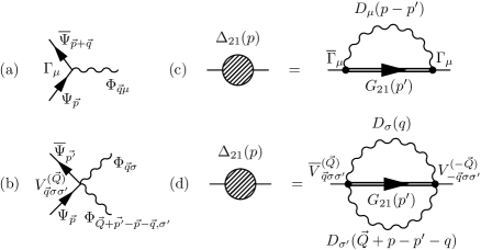
Figure 1: Diagrammatic representations of electron-phonon coupling Hamiltonians (9) and (11) for linear (a) and quadratic (b) couplings respectively. The corresponding self-consistent gap equations (13) and (14) are shown in (c) and (d) respectively.

Similarly to Pisarski & Rischke (1999), we describe the pairing by the set of matrix Green functions in Matsubara representation $G_{ij}(\vec{p},\tau)=-\langle T\Psi^{(i)}_{\vec{p}}(\tau)\overline{\Psi}^{(j)}_{\vec{p}}(0)\rangle$, where $\Psi^{(1)}_{\vec{p}}=\Psi_{\vec{p}}$, $\Psi^{(2)}_{\vec{p}}=\Psi_{\mathrm{C}\vec{p}}\equiv C\overline{\Psi}^{T}_{-\vec{p}}$ is the charge-conjugated spinor and $C=i\gamma^{2}\gamma^{0}$ is the charge-conjugation matrix. The anomalous Green functions $G_{12}$ and $G_{21}$ are responsible for a Cooper pair condensate. The Gor’kov equations, describing the pairing in the mean-field approximation, are:

$$G_{ij}(p)=\delta_{ij}G^{(0)}_{i}(p)+G^{(0)}_{i}(p)\Delta_{i,3-i}(p)G_{3-i,j}(p),$$ (12)

where $p=\{p_{0}=i\pi T(2k+1),\vec{p}\}$, $G^{(0)}_{1,2}(p)=[\gamma^{0}(p_{0}\pm\mu)-v_{\mathrm{F}}\vec{\gamma}\vec{p}]^{-1}$ are the free particle Green functions, following from (1) and $\mu$ is the chemical potential in graphene.

The expressions for the anomalous self-energy $\Delta_{21}$ (the other component $\Delta_{12}=\gamma^{0}\Delta_{21}^{+}\gamma^{0}$) in (12) for the cases of linear (9) and quadratic (11) electron-phonon interaction Hamiltonians are, respectively (see Fig. 1(c,d)),

$$\Delta_{21}(p)=-\frac{T}{S}\sum_{p^{\prime}\mu}g_{\mu}^{2}D_{\mu}(p-p^{\prime})\overline{\Gamma}_{\mu}G_{21}(p^{\prime})\Gamma_{\mu},$$ (13)

$$\Delta_{21}(p)=\frac{2T^{2}}{S^{2}}\sum_{p^{\prime}q}\sum_{\vec{Q}\sigma\sigma^{\prime}}D_{\sigma}(q)D_{\sigma^{\prime}}(\vec{Q}+p-p^{\prime}-q)\overline{V}^{(\vec{Q})}_{\vec{q}\sigma\sigma^{\prime}}G_{21}(p^{\prime})V^{(-\vec{Q})}_{-\vec{q}\sigma\sigma^{\prime}}.$$ (14)

Here the charge-conjugated vertices $\overline{\Gamma}_{\mu}=C^{-1}\Gamma_{\mu}^{T}C$ and $\overline{V}^{(\vec{Q})}_{\vec{q}\sigma\sigma^{\prime}}=C^{-1}V^{(\vec{Q})T}_{\vec{q}\sigma\sigma^{\prime}}C$ are introduced, and $D_{\mu}(q)=2\omega_{\vec{q}\mu}/(q_{0}^{2}-\omega_{\vec{q}\mu}^{2})$ is the phonon Green function.

To solve the Gor’kov equations (12), we assume that the pairing is diagonal with respect to the conduction and valence bands, but suppose, that the structure of the order parameter with respect to electron valleys is parameterized by arbitrary $SU(2)$ matrix. The band-diagonal order parameter can be represented as a decomposition over projection operators $\mathcal{P}_{\pm}(\hat{p})=(1\pm\gamma^{0}\vec{\gamma}\hat{p})/2$ on conduction and valence bands, where $\hat{p}=\vec{p}/|\vec{p}|$ (Pisarski & Rischke 1999). Further, rotation of the order parameter in the valley space can be performed by means of three generators $T_{1}=\gamma^{5}$, $T_{2}=\gamma^{3}\gamma^{5}$ and $T_{3}=i\gamma^{3}$, obeying the algebra of the Pauli matrices (Gusynin et al. 2007). Thus, the explicit form of $\Delta_{21}$ is:

$$\Delta_{21}(p)=e^{i\vec{v}\vec{T}}\left[\Delta_{+}(p)\mathcal{P}_{+}(\hat{p})+\Delta_{-}(p)\mathcal{P}_{-}(\hat{p})\right],$$ (15)

where $\Delta_{\pm}(p)$ are the gaps in conduction and valence bands, and the three-dimensional vector $\vec{v}$ defines the valley structure of the order parameter.

Substituting (15) in (13) and (14), we can derive the system of two coupled gap equations for $\Delta_{\pm}(p)$, having the form:

$$\Delta_{\alpha}(p)=-\frac{T}{S}\sum_{p^{\prime}\beta}\frac{\Delta_{\beta}(p^{\prime})}{p_{0}^{\prime 2}-E^{2}_{\beta}(p^{\prime})}\,\Lambda^{\mu}_{\alpha\beta}(p,p^{\prime};\vec{v}),$$ (16)

where $E_{\pm}(p)=\sqrt{(v_{\mathrm{F}}|\vec{p}|\mp\mu)^{2}+\Delta^{2}_{\pm}(p)}$ are the energies of Bogolyubov excitations in conduction and valence bands. The effective interband ($\alpha=\beta$) and intraband ($\alpha=-\beta$) interactions in the cases of linear and quadratic electron-phonon couplings are, respectively,

$$\Lambda^{\mu}_{\alpha\beta}(p,p^{\prime};\vec{v})=\frac{1}{2}\sum_{\mu}g_{\mu}^{2}D_{\mu}(p-p^{\prime})\,\mathrm{Sp}\left[\mathcal{P}_{\alpha}(\hat{p})e^{-i\vec{v}\vec{T}}\overline{\Gamma}_{\mu}\gamma^{0}e^{i\vec{v}\vec{T}}\mathcal{P}_{\beta}(\hat{p}^{\prime})\gamma^{0}\Gamma_{\mu}\right],$$ (17)

$$\Lambda^{\mu}_{\alpha\beta}(p,p^{\prime};\vec{v})=-\frac{T}{S}\sum_{\vec{q}\vec{Q}}\sum_{\sigma\sigma^{\prime}}D_{\sigma}(q)D_{\sigma^{\prime}}(\vec{Q}+p-p^{\prime}-q)$$

$$\times\mathrm{Sp}\left[\mathcal{P}_{\alpha}(\hat{p})e^{-i\vec{v}\vec{T}}\overline{V}^{(\vec{Q})}_{\vec{q}\sigma\sigma^{\prime}}\gamma^{0}e^{i\vec{v}\vec{T}}\mathcal{P}_{\beta}(\hat{p}^{\prime})\gamma^{0}V^{(-\vec{Q})}_{-\vec{q}\sigma\sigma^{\prime}}\right].$$ (18)

We can find analytical solutions of (16)–(18) in the regime of high doping of graphene, when $\mu$ is greater than the characteristic phonon frequencies. Moreover, high doping facilitates the pairing due to larger density of states at the Fermi level $\mathcal{N}=\mu/2\pi v_{\mathrm{F}}^{2}$. In this case the pairing is effectively one-band, and the Eliashberg equations at $T=0$, following from (16), can be derived by setting $\Delta_{+}(p)=\Delta\Theta(\omega_{0}-p_{0})$, $\Delta_{-}=0$ (similarly to Lozovik et al. 2010):

$$1=2\int\limits_{0}^{\omega_{0}}\frac{d\omega}{\sqrt{\omega^{2}-\Delta^{2}}}\int\limits_{0}^{\infty}d\nu\frac{\alpha^{2}_{\vec{v}}(\nu)F(\nu)}{\omega+\nu}.$$ (19)

Here $\omega_{0}$ is a cutoff frequency of the order of phonon frequencies, and the Eliashberg functions $\alpha^{2}_{\vec{v}}(\nu)F(\nu)$ for in-plane and out-of-plane phonons respectively can be represented as:

$$\alpha^{2}_{\vec{v}}(\nu)F(\nu)=\mathcal{N}g_{\Gamma}^{2}\delta(\nu-\omega_{\Gamma})R^{(1)}_{\Gamma}(\vec{v})+\mathcal{N}g_{\vec{K}}^{2}\delta(\nu-\omega_{\vec{K}})R^{(1)}_{\vec{K}}(\vec{v}),$$ (20)

$$\alpha^{2}_{\vec{v}}(\nu)F(\nu)=Z_{\Gamma}(\nu)R^{(2)}_{\Gamma}(\vec{v})+Z_{\vec{K}}(\nu)R^{(2)}_{\vec{K}}(\vec{v}).$$ (21)

The partial Eliashberg functions of out-of-plane phonons can be calculated within the simple phonon model (see Lozovik & Sokolik (in press)) and reduced to dimensionless functions: $Z_{\mu}(\nu)=(81\mathcal{N}g_{1}^{2}/2a^{2}M^{2}\omega_{\Gamma 2}^{3})\tilde{Z}_{\mu}(x)$, where $x=6\nu/\omega_{\Gamma 2}$, $\omega_{\Gamma 2}\approx 0.11\,\mbox{eV}$. The functions $\tilde{Z}_{\mu}(x)$ are shown in Fig. 2.

Figure 2: Partial dimensionless Eliashberg functions for out-of-plane phonons. Contributions of the two-phonon processes, leaving the electron in its initial valley ($\tilde{Z}_{\Gamma}$, solid line), and flipping it into the opposite valley ($\tilde{Z}_{\vec{K}}$, dotted line) are shown.

Eqs. (20)–(21) show that the Eliashberg functions consist of two parts, corresponding to phonon-mediated electron-electron interaction processes, leaving both electrons in their valleys ($\Gamma$-terms), and flipping both electrons into opposite valleys ($\vec{K}$-terms). The factors $R^{(1,2)}_{\Gamma,\vec{K}}(\vec{v})$, dependent on the valley structure of the order parameter, determine the signs and amplitudes of these contributions:

$$R^{(1)}_{\Gamma}(\vec{v})=-\cos^{2}v+(1-2\hat{v}_{1}^{2})\sin^{2}v,\quad R^{(1)}_{\vec{K}}(\vec{v})=-\cos^{2}v+\hat{v}_{1}^{2}\sin^{2}v,$$

$$R^{(2)}_{\Gamma}(\vec{v})=1,\quad R^{(2)}_{\vec{K}}(\vec{v})=(-\hat{v}_{2}^{2}+\hat{v}_{3}^{2})\sin^{2}v.$$ (22)

All the factors (22) except $R_{\Gamma}^{(2)}$ can vary in the range from $-1$ (the effective phonon-mediated repulsion) to $+1$ (the effective attraction).

The system under pairing conditions should prefer the valley structure $\vec{v}$ of the order parameter, which provides the maximal gap and thus the maximal $\alpha^{2}_{\vec{v}}(\nu)F(\nu)$. For in-plane phonons, the gap, found from (19)–(20), is $\Delta\sim\omega_{\Gamma,\vec{K}}\exp\{-1/\lambda\}$, where the effective coupling constant $\lambda=2\int_{0}^{\infty}(d\nu/\nu)\alpha^{2}_{\vec{v}}(\nu)F(\nu)$ consists of the partial coupling constants: $\lambda=\lambda_{\Gamma}R_{\Gamma}(\vec{v})+\lambda_{\vec{K}}R_{\vec{K}}(\vec{v})$, $\lambda_{\mu}=2\mathcal{N}g_{\mu}^{2}/\omega_{\mu}$. When $\lambda_{\vec{K}}>2\lambda_{\Gamma}$, the preferable pairing structure is $\vec{v}=\{\pi/2,0,0\}$: in this case $R_{\vec{K}}=1$ (scalar and pseudoscalar phonons give rise to effective electron-electron attraction), $R_{\Gamma}=-1$ (pseudovector phonons cause repulsion). At $\lambda_{\vec{K}}<2\lambda_{\Gamma}$, we have $\vec{v}=\{0,(\pi/2)\cos\varphi,(\pi/2)\sin\varphi\}$, and $R_{\Gamma}=1$ (pseudovector phonons cause attraction), $R_{\vec{K}}=0$ (contributions from scalar and pseudoscalar modes cancel each other). Actually, at high values of dielectric permittivity of surrounding medium, $\lambda_{\vec{K}}<2\lambda_{\Gamma}$; at lower permittivity, the Coulomb interaction renormalizes $\lambda_{\vec{K}}$ towards higher values, so the relation $\lambda_{\vec{K}}>2\lambda_{\Gamma}$ can be satisfied (Basko & Aleiner 2008).

For out-of-plane phonons, the preferable valley structure of the order parameter is $\vec{v}=\{0,0,\pi/2\}$, when $R_{\Gamma}=R_{\vec{K}}=1$. Numerical estimates of the coupling constant for out-of-plane phonons show very small values ($10^{-3}$ by the order of magnitude), thus out-of-plane phonons cannot provide any observable electron pairing in graphene. However, in-plane optical phonons can provide observable pairing at heavy doping of graphene.

3 Electron-hole pairing in graphene bilayer

The pairing of spatially separated electrons and holes in graphene bilayer occurs due to Coulomb attraction. This longitudinally-vectorial interaction is described by the vertex $\Gamma=\gamma^{0}$ within the framework of matrix diagrammatic technique, employed in the previous section. Any interaction with such vertex lead to effective electron-electron interaction, independent on the valley structure of the order parameter. Under band-diagonal pairing, the system of self-consistent equations for the conduction- and valence-band gap functions $\Delta_{\pm}(p)$ is similar to (16):

$$\Delta_{\alpha}(p)=-\frac{T}{S}\sum_{p^{\prime}\beta}\frac{1+\alpha\beta\hat{p}\hat{p}^{\prime}}{2}V(|\vec{p}-\vec{p}^{\prime}|,p_{0}-p_{0}^{\prime})\,F_{\beta}(p^{\prime}),$$ (23)

where $F_{\beta}(p^{\prime})=\Delta_{\beta}(p^{\prime})/[p_{0}^{\prime 2}-E_{\beta}^{2}(p^{\prime})]$ is the anomalous Green function and $V(q,\omega)$ is the dynamically screened electron-electron interaction.

The system (23) can be solved in the spirit of BCS theory (Bardeen et al. 1957), i.e. in the static approximation, when one puts $\omega=0$ in $V(q,\omega)$ and assume, that $\Delta_{\pm}(\vec{p},\omega)$ do not depend on $\omega$ and are non-zero in some range of $p$, corresponding to neighborhood of the Fermi surface. Such calculations (Lozovik & Sokolik 2009) showed that in multi-band pairing regime the gap depends exponentially on energy width of the pairing region and thus can be very large. Here we go beyond the static approximation and take into account the frequency dependence of the screened interaction.

The pairing interaction $V(q,\omega)$ can be calculated in the random phase approximation, well-justified in graphene bilayer due to large number of fermionic flavors, equal to 8 (Kharitonov & Efetov 2008a,b; see also Apenko et al. 1982):

$$V(q,\omega)=\frac{v_{q}e^{-qD}}{1-2v_{q}\Pi(q,\omega)+v_{q}^{2}\Pi^{2}(q,\omega)(1-e^{-2qD})},$$ (24)

where $v_{q}=2\pi e^{2}/\varepsilon q$ is the bare Coulomb interaction, $\varepsilon$ is a dielectric permittivity of surrounding medium, $\Pi(q,\omega)$ is a polarization operator of each graphene layer. Hereafter we consider the case of small interlayer distance $D$, when $p_{\mathrm{F}}D\ll 1$, $p_{\mathrm{F}}=\mu/v_{\mathrm{F}}$ is the Fermi momentum. At $\omega=0$, (24) reduces to the statically screened interaction, equal in dimensionless form to $\mathcal{N}V(q,0)=r_{\mathrm{s}}/(q/p_{\mathrm{F}}+8r_{\mathrm{s}})$, where $r_{\mathrm{s}}=e^{2}/\varepsilon v_{\mathrm{F}}\approx 2.19/\varepsilon$ determines the coupling strength. There exist two plasmon branches in the system, corresponding to zeros of denominator of (24): the lower branch with the dispersion $\omega_{-}(q)\approx v_{\mathrm{F}}q$, and the upper branch with the square-root dispersion $\omega_{+}(q)\approx 2\mu\sqrt{r_{\mathrm{s}}(q/p_{\mathrm{F}})}$ at small $q$ and almost linear dispersion at large $q$. When $\omega_{\pm}(q)+v_{\mathrm{F}}q>2\mu$, the plasmons in graphene acquire a finite lifetime due to interband transitions (Wunsch et al. 2006, Hwang & Das Sarma 2007). At $\omega\rightarrow\infty$, the potential $V(q,\omega)$ becomes unscreened: $\mathcal{N}V(q,\infty)=r_{\mathrm{s}}/(q/p_{\mathrm{F}})$.

Using the spectral representations of $F_{\beta}(p^{\prime})$ and $V(q)$ in (23) and summing over $p_{0}^{\prime}$ at $T=0$, we get the Eliashberg-type equations:

$$\Delta_{\alpha}(\vec{p},\omega)=-\sum_{\beta}\int\frac{d\vec{p^{\prime}}}{(2\pi)^{2}}\frac{1+\alpha\beta\hat{p}\hat{p}^{\prime}}{2}\int\limits_{0}^{\infty}\frac{d\omega^{\prime}}{\pi}\,\mathrm{Im}F_{\beta}(\vec{p^{\prime}},\omega^{\prime})\left\{v_{\vec{p}-\vec{p^{\prime}}}+\int\limits_{0}^{\infty}\frac{d\nu}{\pi}\right.$$

$$\left.\vphantom{\int\limits_{0}^{\infty}}\times\mathrm{Im}V(\vec{p}-\vec{p^{\prime}},\omega-\omega^{\prime}+i\delta)\left(\frac{1}{\omega^{\prime}+\nu+\omega+i\delta}-\frac{1}{\omega^{\prime}+\nu-\omega-i\delta}\right)\right\}.$$ (25)

We assume that $\Delta(\vec{p},\omega)$ is real (it is well-justified near $\omega=0$), therefore $\mathrm{Im}F_{\beta}(p^{\prime})=-\pi\delta(\omega^{\prime}-E_{\beta}(p^{\prime}))\Delta_{\beta}(p^{\prime})/2E_{\beta}(p^{\prime})$. Then, we assume that the argument of the $\delta$-function in this expression vanishes at some unambiguous $\omega^{\prime}=\tilde{\omega}(\vec{p^{\prime}})$. This allows us to handle only “on-shell” gap functions and Bogolyubov energies: $\Delta_{\alpha}(|\vec{p}|)\equiv\Delta_{\alpha}(\vec{p},\tilde{\omega}(\vec{p}))$, $E_{\alpha}(|\vec{p}|)\equiv E_{\alpha}(\vec{p},\tilde{\omega}(\vec{p}))$. Rewriting (25) in terms of the on-shell quantities and assuming $\alpha=+1$, $p=p_{\mathrm{F}}$ in its left-hand side, we get:

$$\Delta_{+}(p_{\mathrm{F}})=\sum_{\beta}\int\frac{d\vec{p^{\prime}}}{(2\pi)^{2}}\frac{1+\beta\hat{p}\hat{p}^{\prime}}{2}\frac{\Delta_{\beta}(p^{\prime})}{2E_{\beta}(p^{\prime})}$$

$$\times\left\{v_{\vec{p}-\vec{p^{\prime}}}+\frac{2}{\pi}\int\limits_{0}^{\infty}\mathrm{Im}V(\vec{p}-\vec{p^{\prime}},\nu+i\delta)\frac{d\nu}{E_{\beta}(p^{\prime})+\nu}\right\}.$$ (26)

Here we also neglected $\omega=\Delta_{+}(p_{\mathrm{F}})$ in the second term in the braces.

To demonstrate the influence of dynamical screening of $V(q,\omega)$ on the gap value, we will simplify the equation (26) further. Firstly, we suppose that the both on-shell gap functions $\Delta_{\beta}(p)$ are equal to each other; this seems plausible at large $r_{\mathrm{s}}$, as discussed by Lozovik & Sokolik 2010, and allows us to neglect the angular factor $\hat{p}\hat{p}^{\prime}$ in (26). Secondly, we assume $\Delta_{\pm}(p)=\Delta f(p)$, where $\Delta=\Delta_{+}(p_{\mathrm{F}})$ is the gap at the Fermi surface and $f(p)$ is some trial function, equal to 1 at $p=p_{\mathrm{F}}$ and having the asymptotics $f(p)\propto 1/p$ at $p\rightarrow\infty$, caused by the leading contribution of the unscreened Coulomb interaction in (25). For computational purposes, it is also convenient to single out the contribution of undamped plasmons of the higher branch as: $\mathrm{Im}V(q,\nu+i\delta)=\mathrm{Im}V(q,\nu)-\pi\delta[\nu-\omega_{+}(q)]A(q)$. Here the spectral weight of the higher branch plasmons is $A(q)=-v_{q}/2[\partial\Pi(q,\omega)/\partial\omega]|_{\omega=\omega_{+}(q)}$ when $q+\omega_{+}(q)<2\mu$ and zero otherwise. Thus, the equation (26) for the gap reduces to:

$$1=\frac{1}{2}\sum_{\beta}\int\frac{d\vec{p}}{(2\pi)^{2}}\frac{\Delta_{\beta}(p)}{2E_{\beta}(p)}\left\{v_{\vec{p}-\vec{p}_{\mathrm{F}}}-\frac{2A(\vec{p}-\vec{p}_{\mathrm{F}})}{E_{\beta}(p)+\omega_{+}(\vec{p}-\vec{p}_{\mathrm{F}})}+\vphantom{\int\limits_{0}^{\infty}}\right.$$

$$\left.+\frac{2}{\pi}\int\limits_{0}^{\infty}\mathrm{Im}V(\vec{p}-\vec{p}_{\mathrm{F}},\nu)\frac{d\nu}{E_{\beta}(p)+\nu}\right\}.$$ (27)

Figure 3: On-shell interaction, represented by the expression in the braces of (27), in the intraband channel ($\beta=+1$) at $r_{\mathrm{s}}=2$. Solid line: full on-shell interaction, dash-dotted line: unscreened Coulomb interaction only, dotted line: unscreened Coulomb interaction with the contribution of undamped plasmons, dashed line: statically screened interaction.

The expression in braces in (27) is the effective on-shell interaction, which incorporates the effects of dynamical screening of the pairing interaction. It differs from the statically screened interaction $V(q,\omega)$, employed by Lozovik & Sokolik 2009, Lozovik & Sokolik 2010 and is naturally divided into three contributions (see Fig. 3): a) attractive unscreened Coulomb interaction, b) repulsive contribution due to virtual undamped higher-branch plasmons, c) repulsive contribution due to virtual damped higher-branch plasmons and single-particle intra- and interband excitation continuums at $\omega<v_{\mathrm{F}}q$ and $\omega+v_{\mathrm{F}}q>2\mu$ respectively (Wunsch et al. 2006, Hwang & Das Sarma 2007). However, strictly on the Fermi surface (at $\beta=+1$, $p=p_{\mathrm{F}}$) the effective on-shell interaction coincides with the statically-screened one.

Assuming that the characteristic momentum, at which the on-shell gap $\Delta_{\pm}(p)$ decays, is of the order of the Fermi momentum and employing $f(p)=p_{\mathrm{F}}/(|p-p_{\mathrm{F}}|+p_{\mathrm{F}})$ as a trial function, we can study the influence of dynamical screening of the pairing interaction on the gap value $\Delta$. Fig. 4 shows the results of the numerical solution of (27) with taking into account various contributions to the effective on-shell interaction. Taking into account only the unscreened Coulomb attraction results in huge gap values, reported previously by Min et al. (2008), Zhang & Joglekar (2008). The addition of the undamped plasmons repulsive contribution eliminates the logarithmic singularity of the effective interaction on the Fermi momentum (Fig. 3), but do not change the gap values essentially at large $r_{\mathrm{s}}$. Finally, the contribution of the damped plasmons and and single-particle excitations lowers the gap down to the values of the order of $0.01\mu$ at maximum (several Kelvins at $\mu\sim 0.1\,\mbox{eV}$).

Figure 4: Values of the gap at the Fermi surface $\Delta$, normalized on the chemical potential $\mu$, as functions of $r_{\mathrm{s}}$, calculated with taking into account various contributions to the effective on-shell interaction. Solid line: full on-shell interaction, dash-dotted line: unscreened Coulomb interaction only, dotted line: unscreened Coulomb interaction with the contribution of undamped plasmons, dashed line: statically screened interaction.

When the on-shell interaction is replaced by the statically screened one $V(q,0)$, the gap is unobservably small, if we use the trial function $f(p)$, spread over the momentums of the order of $p_{\mathrm{F}}$; this is in argeement with the BCS-type estimates by Kharitonov & Efetov (2008a,b). However, as shown by Lozovik & Sokolik (2009), the pairing tend to occupy much larger region of the momentums of the order of $8r_{\mathrm{s}}p_{\mathrm{F}}$ and results in large gap values, if we use the statically screened potential as the pairing potential. In our case, when we take into account the dynamical effects and naturally assume that the on-shell gaps $\Delta_{\pm}(p)$ decay at $p\sim p_{\mathrm{F}}$, the gap turns out to take the values, several orders of magnitude smaller than these with unscreened Coulomb interaction, but, at the same time, several orders of magnitude larger than the BCS-type estimates.

4 Conclusions

We have considered electron-electron pairing in graphene, mediated by in-plane and out-of-plane phonons, and electron-hole pairing in graphene bilayer, mediated by the screened Coulomb interaction. In both cases we consider the generally multi-band pairing with the $s$-wave order parameter, diagonal with respect to valence and conduction bands of paired particles. Moreover, we take into account the frequency dependence of pairing interaction in both cases, deriving and solving two-band Eliashberg-type equations.

The consideration of phonon-mediated pairing is performed by resolution of electron-phonon interaction with respect to sublattice and valley degrees of freedom of electrons in graphene and taking into account a possibility of different structures of the order parameter in valley space. We demonstrate that contributions of different phonon modes in graphene to effective electron-electron interaction, entering the Eliashberg-type equations, depend both on symmetries of these modes and on the structure of the order parameter in valley space.

The coupling of graphene electrons with out-of-plane (flexural) phonon modes is quadratic and leads to unusual form of effective electron-electron phonon-mediated interaction, which includes integration on frequency and integration on momentum over the whole Brillouin zone within the phonon loop. The estimates of effective coupling constants show that the pairing due to in-plane phonon modes can occur at high doping of graphene, while the pairing due to out-of-plane phonons does not occur at observable temperatures.

Eliashberg-type equations for electron-hole pairing in graphene bilayer, written in the present paper in terms of the “on-shell” gap functions, allow to estimate the role of dynamical effects. The effective on-shell dynamically screened interaction, entering the gap equations, can be represented as a sum of attractive unscreened Coulomb interaction, repulsive contribution due to undamped virtual plasmons and combined repulsive contribution of the damped plasmons and of the continuum of single-particle excitations.

The unscreened Coulomb interaction on its own provides large values of the gap, which are only slightly reduced with taking into account the undamped plasmons. Inclusion of the damped plasmons and single-particle excitations lower down the gap by several orders of magnitude. This result demonstrates the significant competition between the bare Coulomb attraction and virtual excitations in the system, responsible for its dynamical screening. However, the estimates of the gap, calculated with taking into account the full on-shell potential, are by several orders of magnitude larger than the BCS-type estimates and can reach several Kelvins at strong coupling.

References

- [1]
- [2] Apenko, S.M., Kirzhnits, D.A. & Lozovik, Yu.E. 1982 On the validity of the 1/N expansion. Phys. Lett. A 92, 107–109. (doi:10.1016/0375-9601(82)90343-7)
- [3]
- [4] Armour, W., Hands, S. & Strouthos, C. 2009 Lattice simulations near the semimetal-insulator phase transition of graphene. (http://arxiv.org/abs/cond-mat/0908.0118v1)
- [5]
- [6] Bardeen, J., Cooper, L.N. & Schrieffer, J.R. 1957 Theory of superconductivity Phys. Rev. 108, 1175–1204. (doi:10.1103/PhysRev.108.1175)
- [7]
- [8] Basko, D.M. & Aleiner, I.L. 2008 Interplay of Coulomb and electron-phonon interactions in graphene Phys. Rev. B 77, 041409(R). (doi:10.1103/PhysRevB.77.041409)
- [9]
- [10] Beenakker, C.W.J. 2008 Andreev reflection and Klein tunneling in graphene Rev. Mod. Phys. 80, 1337–1354. (doi:10.1103/RevModPhys.80.1337)
- [11]
- [12] Berman, O.L., Lozovik, Yu.E. & Gumbs, G. 2008a Bose-Einstein condensation and superfluidity of magnetoexcitons in bilayer graphene. Phys. Rev. B 77, 155433. (doi:10.1103/PhysRevB.77.155433)
- [13]
- [14] Berman, O.L., Kezerashvili, R.Ya. & Lozovik, Yu.E. 2008b Collective properties of magnetobiexcitons in quantum wells and graphene superlattices. Phys.Rev. B 78, 035135. (doi:10.1103/PhysRevB.78.035135)
- [15]
- [16] Black-Schaffer, A.M. & Doniach, S. 2007 Resonating valence bonds and mean-field d-wave superconductivity in graphite. Phys. Rev. B 75, 134512. (doi:10.1103/PhysRevB.75.134512)
- [17]
- [18] Castro Neto, A.H., Guinea, F., Peres, N.M.R., Novoselov, K.S. & Geim, A.K. 2009 The electronic properties of graphene. Rev. Mod. Phys. 81, 109–162. (doi:10.1103/RevModPhys.81.109)
- [19]
- [20] Drut, J.E. & Lähde, J.A. 2008 Is graphene in vacuum an insulator? Phys. Rev. Lett. 102, 026802. (doi:10.1103/PhysRevLett.102.026802)
- [21]
- [22] González, J. 2008 Kohn-Luttinger superconductivity in graphene. Phys. Rev. B 78, 205431. (doi:10.1103/PhysRevB.78.205431)
- [23]
- [24] Gusynin V.P., Sharapov, S.G. & Carbotte, J.P. 2007 AC conductivity of graphene: from tight-binding model to 2+1-dimensional quantum electrodynamics. Int. J. Mod. Phys. B 21, 4611–4658. (doi:10.1142/S0217979207038022)
- [25]
- [26] Heersche, H.B., Jarillo-Herrero P., Oostinga, J.O., Vandersypen, L.M.K. & Morpurgo, A.F. 2007 Bipolar supercurrent in graphene. Nature, 446, 56–59. (doi:10.1038/nature05555)
- [27]
- [28] Honerkamp C. 2008 Density waves and Cooper pairing on the honeycomb lattice Phys. Rev. Lett. 100, 164404. (doi:10.1103/PhysRevLett.100.146404)
- [29]
- [30] Hwang, E.H. & Das Sarma, S. 2007 Dielectric function, screening, and plasmons in two-dimensional graphene. Phys. Rev. B 75, 205418. (doi:10.1103/PhysRevB.75.205418)
- [31]
- [32] Katsnelson, M.I., Novoselov, K.S. & Geim, A.K. 2006 Chiral tunnelling and the Klein paradox in graphene. Nature Phys. 2, 620–625. (doi:10.1038/nphys384)
- [33]
- [34] Katsnelson, M.I. & Novoselov, K.S. 2007 Graphene: new bridge between condensed matter physics and quantum electrodynamics. Solid State Commun. 143, 3–13. (doi:10.1016/j.ssc.2007.02.043)
- [35]
- [36] Kharitonov, M.Yu. & Efetov, K.B. 2008a Electron screening and excitonic condensation in double-layer graphene systems. Phys. Rev. B 78, 241401(R). (doi:10.1103/PhysRevB.78.241401)
- [37]
- [38] Kharitonov, M.Yu. & Efetov, K.B. 2008b Excitonic condensation in a double-layer graphene system. Semicond. Sci. Tech. 25, 034004. (doi:10.1088/0268-1242/25/3/034004)
- [39]
- [40] Khveshchenko, D.V. 2001 Ghost excitonic insulator transition in layered graphite. Phys. Rev. Lett. 87, 246802. (doi:10.1103/PhysRevLett.87.246802)
- [41]
- [42] Khveshchenko, D.V. 2009 Massive Dirac fermions in single-layer graphene. J. Phys.: Condens. Matter 21, 075303. (doi:10.1088/0953-8984/21/7/075303)
- [43]
- [44] Lozovik, Yu.E. & Berman, O.L. 1997 Phase transitions in a system of spatially separated electrons and holes. JETP 84, 1027–1035. (doi:10.1134/1.558220)
- [45]
- [46] Lozovik, Yu.E. & Sokolik, A.A. 2008a Electron-hole pair condensation in a graphene bilayer. JETP Lett. 87, 55–59. (doi:10.1134/S002136400801013X)
- [47]
- [48] Lozovik, Yu.E. & Sokolik 2008b Coherent phases and collective electron phenomena in graphene. J. Phys.: Conf. Ser. 129, 012003. (doi:10.1088/1742-6596/129/1/012003)
- [49]
- [50] Lozovik, Yu.E., Merkulova, S.P. & Sokolik, A.A. 2008 Collective electron phenomena in graphene. Phys.-Usp. 51, 727-744. (doi: 10.1070/PU2008v051n07ABEH006574)
- [51]
- [52] Lozovik, Yu.E. & Sokolik, A.A. 2009 Multi-band pairing of ultrarelativistic electrons and holes in graphene bilayer. Phys. Lett. A 374, 326–330. (doi:10.1016/j.physleta.2009.10.045)
- [53]
- [54] Lozovik, Yu.E., Ogarkov, S.L. & Sokolik, A.A. 2010 Theory of superconductivity for Dirac electrons in graphene. JETP 110, 49–57. (doi:10.1134/S1063776110010073)
- [55]
- [56] Lozovik, Yu.E. & Poushnov, A.V. 1997 Magnetism and Josephson effect in a coupled quantum well electron-hole system. Phys. Lett. A 228, 399–407. (doi:10.1016/S0375-9601(97)00133-3)
- [57]
- [58] Lozovik, Yu.E. & Sokolik, A.A. 2010 Ultrarelativistic electron-hole pairing in graphene bilayer. Eur. Phys. J. B 73, 195–206. (doi:10.1140/epjb/e2009-00415-9)
- [59]
- [60] Lozovik, Yu.E. & Sokolik, A.A. In press. Phonon-mediated electron pairing in graphene. Phys. Lett. A
- [61]
- [62] Lozovik, Yu.E. & Yudson, V.I. 1975 Feasibility of superfluidity of paired spatially separated electrons and holes; a new superconductivity mechanism. JETP Lett. 22, 274–276.
- [63]
- [64] Lozovik, Yu.E. & Yudson, V.I. 1976 Superconductivity at dielectric pairing of spatially separated quasiparticles. Sol. St. Commun. 19, 391–393. (doi:10.1016/0038-1098(76)91360-0)
- [65]
- [66] Mariani, E. & von Oppen, F. 2008 Flexural phonons in free-standing graphene. Phys. Rev. Lett. 100, 076801. (doi:10.1103/PhysRevLett.100.076801)
- [67]
- [68] Min, H., Bistritzer, R., Su, J.-J. & MacDonald, A.H. 2008 Room-temperature superfluidity in graphene bilayers. Phys. Rev. B 78, 121401(R). (doi:10.1103/PhysRevB.78.121401)
- [69]
- [70] Nozières, P. & Schmitt-Rink S. 1985 Bose condensation in an attractive fermion gas: from weak to strong coupling superconductivity. J. Low Temp. Phys. 59, 195–211. (doi:10.1007/BF00683774)
- [71]
- [72] Pisarski, R.D. & Rischke, D.H. 1999 Superfluidity in a model of massless fermions coupled to scalar bosons. Phys. Rev. D 60, 094013. (doi:10.1103/PhysRevD.60.094013)
- [73]
- [74] Piscanec, S., Lazzeri, M., Mauri, F., Ferrari, A.C. & Robertson, J. 2004 Kohn anomalies and electron-phonon interactions in graphite. Phys. Rev. Lett. 93, 185503. (doi:10.1103/PhysRevLett.93.185503)
- [75]
- [76] Sabio, J., Sols F. & Guinea F. Two-body problem in graphene. Phys. Rev. B 81, 045428. (doi:10.1103/PhysRevB.81.045428)
- [77]
- [78] Shevchenko, S.I. 1994 Phase diagram of systems with pairing of spatially separated electrons and holes. Phys. Rev. Lett. 72, 3242–3245. (doi:10.1103/PhysRevLett.72.3242)
- [79]
- [80] Suzuura, H. & Ando, T. 2002 Phonons and electron-phonon scattering in carbon nanotubes. Phys. Rev. B 65, 235412. (doi:10.1103/PhysRevB.65.235412)
- [81]
- [82] Uchoa ,B. & Castro Neto, A.H. 2007 Superconducting states of pure and doped graphene. Phys. Rev. Lett. 98, 146801. (doi:10.1103/PhysRevLett.98.146801)
- [83]
- [84] Wunsch, B., Stauber, T., Sols, F. & Guinea, F. 2006 Dynamical polarization of graphene at finite doping. New J. Phys. 8, 318. (doi:10.1088/1367-2630/8/12/318)
- [85]
- [86] Zhang, C.-H. & Joglekar, Y.N. 2008 Excitonic condensation of massless fermions in graphene bilayers. Phys. Rev. B 77, 233405. (doi:10.1103/PhysRevB.77.233405)
- [87]