Monte Carlo simulation of joint density of states of two continuous spin models using Wang-Landau-Transition-Matrix Algorithm

Abstract

Monte Carlo simulation has been performed in one-dimensional Lebwohl-Lasher model and two dimensional XY-model using the Wang-Landau and the Wang-Landau-Transition-Matrix Monte Carlo methods. Random walk has been performed in the two-dimensional space comprising of energy-order parameter and energy-correlation function and the joint density of states (JDOS) were obtained. From the JDOS the order parameter, susceptibility and correlation function are calculated. Agreement between the results obtained from the two algorithms is very good.

PACS: 64.60.De; 61.30.-v; 05.10.Ln
Keywords: Wang Landau, Transition Matrix. Joint Density of states

I Introduction

During the last couple of years or so a number of Monte-Carlo (MC) algorithms have been proposed which directly determine the density of states (DOS) of a system. One of these is the Transition Matrix Monte Carlo (TMMC) algorithm developed by Oliveria et al oliveria1 and subsequently generalized by Wang and co-workers swendsen . In this algorithm, during a random walk in the energy space, one keeps a record of the transitions between the microstates of the system. The entire history of the transitions is then used to obtain the density of states of the system. More recently Wang and Landau wlprl proposed another algorithm which goes by their name (WL) and has drawn wide attention of investigators. This algorithm employs a method of flat histograms, while a random walk is performed in the energy space and estimates the DOS of the system by using an iterative scheme. Both methods, the TMMC and WL, depend on broad sampling of the phase space and are easy to implement. A knowledge of the DOS of a system as a function of energy, $\Omega(E)$ enables one to calculate the partition function $Z$ by a simple Boltzmann reweighting: $Z(\beta)={\displaystyle\sum_{E}{\Omega(E)e^{-\beta E}}}$, where $\beta$ is the inverse temperature $1/T$. With a knowledge of the partition function one can calculate the averages of thermodynamic quantities which are directly related to energy. It has been established that while the TMMC method gives more accurate estimation of the DOS, the WL algorithm is more efficient in sampling the phase space.
Shell et al proposed shell an algorithm which is an amalgamation of the two algorithms and utilizes the benefits of each. This algorithm, now known as the Wang Landau Transition Matrix (WLTM) Monte Carlo algorithm, is at the same time efficient and accurate. Shell et al applied the algorithm to a two-dimensional Ising model and a Lennard-Jones fluid. More recently Ghulghazarya et al ghulgha have applied this method to simulate protein and peptide.
The sampling of the phase space which is done in each of the above methods need not be restricted to the evaluation of the density of states as a function of energy alone. One can determine the DOS or to be more specific, the Joint Density of States (JDOS) with a substantially more book-keeping. The JDOS $\Omega(E,\phi)$ is a function of some variable $\phi$ (which can be an order parameter, spin-spin correlation or any other observable) besides the energy $E$. This partition function is determined from: $Z(\beta)={\displaystyle\sum_{E}\sum_{\phi}{\Omega(E,\phi)e^{-\beta E}}}$. The ensemble average of any function of $\phi$ at an inverse temperature $\beta$ is then given by

$$<f(\phi,\beta)>=\frac{{\displaystyle\sum_{E}\sum_{\phi}f(\phi)\Omega(E,\phi)e^{-\beta E}}}{{\displaystyle\sum_{E}\sum_{\phi}\Omega(E,\phi)e^{-\beta E}}}$$ (1)

Most of the investigators have so far worked on the determination of DOS or JDOS in discrete systems using the three above mention algorithms shell2 ; yan ; landau ; xu ; kisor . Even in this domain the amount of work reported on the determination of JDOS is relatively small. In an earlier paper shyamal we have reported on the working of WLTM in two continuous lattice-spin models. While the discrete systems like Ising or Potts model can be handled in a straight forward manner, the investigation of continuous systems are more tedious. The range of energy (and another observable in case of two-dimensional random walk) needs to be discretized and several parameters appear which are to be chosen properly for the determination of DOS or JDOS. In the present communication we report the determination of JDOS using the WLTM algorithm in two continuous lattice spin models. The quantities evaluated other than energy and specific heat are the order parameter, susceptibility and correlation function. One of the models is the one-dimensional Lebwohl-Lasher model ll , which is exactly solvable romerio and therefore allows us to check the accuracy of the results of our simulation. The other system is the two-dimensional XY-model where exact solutions are not available and we have compared the results with those obtained from the JDOS determined using the WL algorithm. The aim of the present work is to test the feasibility of the determination of JDOS in continuous models using the WLTM algorithm. This turned out to be a some what difficult task as a formidable amount of computer memory is necessary even for systems of moderate size.

II The different algorithms

II.1 The Wang Landau algorithm

We outline below the method of determination of the JDOS, $\Omega(E,\phi)$ using the WL algorithm. In a system where $E$ and $\phi$ are continuous variables, discretization in required to label the macrostates of the system. The ranges of $E$ and $\phi$ are divided into a large number of bins of width $d_{e}$ and $d_{\phi}$ respectively. Let $E_{I}$ and $\phi_{J}$ be the mean energy and mean order parameter (or correlation function) corresponding to the $I^{th}$ bin of energy and the $J^{th}$ bin of the order parameter (correlation function) respectively. Then $\Omega(I,J)$ denotes the number of microstates of the system having energy $E_{I}$ and order parameter (correlation function) $\phi_{J}$ or simply the degeneracy of the macrostate $(I,J)$. Since $\Omega(I,J)$ is a very large number, it is convenient to work with its natural logarithm and we use $g(I,J)=ln\Omega(I,J)$.

We perform two dimensional random walk in the $(E-\phi)$ space. Initially we do not have any knowledge of $g(I,J)$, and set $g(I,J)=0$ for all values of $I$ and $J$. Also, an histogram count $H(I,J)$ of the states visited during the random walk is maintained. The WL algorithm generates the JDOS profile, which progressively approaches the actual density of states of the system. The algorithm starts with some microstate of the system and successive microstates are generated by rotating one spin at a time. Let $(I,J)$ and $(K,L)$ be the macrostates before and after rotating the spin and the corresponding microstates are $(i,j)$ and $(k,l)$, where $i\in I,j\in J$ and $k\in K,l\in L$. The transition probability from state $(i,j)$ to $(k,l)$ is given by

$$P(i,j\rightarrow k,l)=min\left(\frac{\Omega(I,J)}{\Omega(K,L)},1\right)$$ (2)

Thus the acceptance probability of the new state is inversely proportional to the current density of states. When the new state is accepted the density of states $g(K,L)$ and the histogram count $H(K,L)$ of the state $(K,L)$ are modified as

$$g(K,L)=g(K,L)+lnf$$ (3a)

$$\text{and}\qquad H(K,L)=H(K,L)+1$$ (3b)

and when the new state is not accepted the old density of state $g(I,J)$ and histogram count $H(I,J)$ are modified as

$$g(I,J)=g(I,J)+lnf$$ (4a)

$$\text{and}\qquad H(I,J)=H(I,J)+1$$ (4b)

Here $f$ is a modification factor whose initial value was chosen to be equal to $e$. When the histogram is sufficiently flat (say, 80%) i.e., histogram count $H(I,J)$ of each bin $(I,J)$ is at least $80\%$ of the mean histogram $H_{M}=\left(\sum^{M_{1}}_{I}\sum^{M_{2}}_{J}H(I,J)\right)/M$ , $M$ being the total number of bins then one iteration is said to be complete. Then the histogram is reset to zero for all values of $I$ and $J$ and the modification factor $f$ is reduced in some prescribed manner (we use $lnf\rightarrow lnf/2$). A fresh iteration is started with the modified value of $lnf$ and the old values of $g(I,J)^{\prime}s$ which were calculated in the previous iteration. One continues iterations with the same procedure until the modification factor becomes sufficiently small (say, $10^{-8}$). The error introduced in the joint density of states has been predicted to be proportional to $\sqrt{(}lnf)$ as is apparent from the theoretical work of Zhou and Bhatt zhou . This has been tested for a number of discrete and continuous models and the prediction has been found to be correct lee .

II.2 The Transition Matrix Monte Carlo algorithm

The TMMC algorithm is an efficient algorithm in which one directly calculates the density of states and was first proposed by Oliveria et al. in the year 1996. If the transition probability from a microstate $(i,j)$ to another microstate $(k,l)$ is $t(i,j;k,l)$ and that from a macrostate $(I,J)$ to a macrostate $(K,L)$ is $T(I,J;K,L)$ then

$$T(I,J;K,L)=\frac{1}{\Omega(I,J)}\sum_{i\in I}\sum_{j\in J}\sum_{k\in K}\sum_{l\in L}{t(i,j;k,l)}$$ (5)

with the following conditions:

$$\sum_{k,l}{t(i,j;k,l)}=1,\qquad t(i,j;k,l)\geq 0$$ (6a)

$$\text{and}\qquad\sum_{K,L}{T(I,J;K,L)}=1,\qquad T(I,J;K,L)\geq 0$$ (6b)

If $T(K,L;I,J)$ be the reverse transition then one can write

$$\frac{T(I,J;K,L)}{T(K,L;I,J)}=\frac{\Omega(K,L)}{\Omega(I,J)}\frac{\displaystyle{\sum_{i\in I}\sum_{j\in J}\sum_{k\in K}\sum_{l\in L}{t(i,j;k,l)}}}{\displaystyle{\sum_{k\in K}\sum_{l\in L}\sum_{i\in I}\sum_{j\in J}{t(k,l;i,j)}}}$$ (7)

The transition probability $t(i,j;k,l)$ actually is a product of two probabilities,

$$t(i,j;k,l)=a(i,j;k,l)P(i,j;k,l)$$ (8)

Here $a(i,j;k,l)$ is the probability of the move $(i,j)\rightarrow(k,l)$ being proposed and depends on the type of the Monte Carlo moves and while $P(i,j;k,l)$ is the probability of proposed move being accepted and depends on the configurations $(i,j)$ and $(k,l)$. One can choose any value of $P$ and an infinite temperature transition probability $(T_{\infty})$ can be chosen for which $P(i,j;k,l)=1$ for all i,j and k,l. This is particularly easy to understand if one considers the Metropolis algorithm at infinite temperature. This process does not affect the JDOS to be determined since it is independent of temperature. Using equations (7) and (8) we can write:

$$\frac{T_{\infty}(I,J;K,L)}{T_{\infty}(K,L;I,J)}=\frac{\Omega(K,L)}{\Omega(I,J)}\frac{\displaystyle{\sum_{i\in I}\sum_{j\in J}\sum_{k\in K}\sum_{l\in L}a(i,j;k,l)}}{\displaystyle{\sum_{k\in K}\sum_{l\in L}\sum_{i\in I}\sum_{j\in J}a(k,l;i,j)}}$$ (9)

Again for symmetric moves (single spin flip dynamics) $a(i,j;k,l)=a(k,l;i,j)$ and the summation terms on right hand side of equation (9) drops out and the equation can be simplified as

$$\frac{T_{\infty}(I,J;K,L)}{T_{\infty}(K,L;I,J)}=\frac{\Omega(K,L)}{\Omega(I,J)}$$ (10)

This equation relates the JDOS with the infinite temperature transition probabilities. Thus from the knowledge of infinite temperature transition probabilities one can estimate the JDOS. Now, one needs to calculate $T_{\infty}$(I,J;K,L) which can be done by keeping a record of moves in the form of a matrix, called C-matrix, $C(I,J;K,L)$ for all proposals $(I,J)\rightarrow(K,L)$, during the random walk. Initially, we set $C(I,J;K,L)=0$ for all I,J and K,L. At infinite temperature all the proposed moves are accepted so whenever a move is proposed we update the C-matrix as

$$C(I,J;K,L)=C(I,J;K,L)+1$$ (11)

Once the construction of C-matrix is started we never reset it to zero, because the C-matrix keeps the detail history of the transitions in the system. The current estimate of the infinite temperature transition probability ($\widetilde{T}_{\infty}$) is

$$\widetilde{T}_{\infty}(I,J;K,L)=\frac{C(I,J;K,L)}{\displaystyle{\sum_{K}\sum_{L}C(I,J;K,L)}}$$ (12)

Where the sum extends over all $K$ and $L$ and the tilde indicates the estimate. From equation (10) and (12) one can determine the joint density of states. But the equation (10) is an over specified problem since for a system with $N$ macrostate having $N$ unknown quantities $\Omega(I,J)$ there are $N(N-1)/2$ such equations. To calculate $\Omega(I,J)$ one needs to minimize the total variance

$$\sigma^{2}_{tot}=\sum_{I,J;K,L}{\displaystyle{\frac{[S(I,J)-S(K,L)+ln\left(\frac{\widetilde{T}_{\infty}(I,J;K,L)}{\widetilde{T}_{\infty}(K,L;I,J)}\right)]^{2}}{\sigma^{2}_{IJKL}}}}$$ (13)

with

$$\sigma^{2}_{IJKL}=C(I,J;K,L)^{-1}+H(I,J)^{-1}+C(K,L;I,J)^{-1}+H(K,L)^{-1}$$ (14)

Here we have used $S(I,J)=ln\Omega(I,J)$ and $H(I,J)=\sum_{K,L}C(I,J;K,L)$. In order to ensure that the random walker visits all macrostates in the region of interest one considers a uniform ensemble, where all macrostates are equally probable. The probability of occurrence of a given microstate $(i,j)$ is therefore proportional to the multiplicity of the macrostate $(I,J)$ where $i\in I$ and $j\in J$. So the probability of acceptance of a move $(i,j)\rightarrow(k,l)$ is given by

$$p(i,j\rightarrow k,l)=min\left(1,\frac{\Omega(I,J)}{\Omega(K,L)}\right)$$ (15)

Since the JDOS are not known a priori, the acceptance criteria can be written as

$$p(i,j\rightarrow k,l)=min\left(1,\frac{\widetilde{T}_{\infty}(K,L;I,J)}{\widetilde{T}_{\infty}(I,J;K,L)}\right)$$ (16)

where we have used equation (10) So using the above acceptance probability together with equation (10) and minimizing the total variance as discussed above, one can generate the profile of the joint density of states. The TMMC algorithm gives accurate value of JDOS since it stores and uses the entire history of the transitions during the random walk. But this method has a drawback that the convergence is not guaranteed and a significant amount of CPU time is necessary. On the other hand the WL method ensures that all the macrostates are visited rather efficiently and more quickly. As proposed by Shell and co-workers shell in the WLTM method we combine the TMMC and WL algorithms in order to get the benefit of both the algorithms. This is discusses in the next section.

II.3 Combination of Wang-Landau and Transition Matrix Monte Carlo algorithm: The WLTM algorithm

In the WLTM algorithm, one efficiently combines the WL and TM Monte Carlo algorithms. In this algorithm, the phase space is sampled via the acceptance criteria given by equation (15) as in the WL method. Also $g(I,J)$ and $H(I,J)$ are updated in the same fashion as in the WL algorithm and in addition of these, a record of transitions between macrostates is kept in a C-matrix, which is never zeroed during the simulation. At the end of the simulation, from the knowledge of the C-matrix and using equation (10) the joint density of states is determined by minimizing the total variance.

III The models used in the present work

We have determined the JDOS and other thermodynamic quantities such as energy, specific heat, order parameter, correlation function etc. performing two dimensional random walk in $E-\phi$ space using WL and WLTM algorithms for two continuous lattice spin models. We give below a brief description of the models and the related quantities we have measured.

III.1 The 1-d Lebwohl-Lasher model

This model is a linear array of three dimensional spins $(d=1,n=3)$ interacting with nearest neighbors via the a potential

$$V_{ij}=-P_{2}(cos\theta_{ij})$$ (17)

Where $P_{2}$ is the second Legendre polynomial and $\theta_{ij}$ is the angle between two nearest neighbor spins $i$ and $j$. Spins are headless, i.e. it has O(3) as well as $Z_{2}$ symmetry. This model represents one dimensional nematic liquid crystal and does not exhibit any finite temperature order disorder phase transition.
The order parameter is a quantity which describes the amount of order prevailing in a system. Since in a nematic phase the ordering is the orientational, the order parameter quantifies the amount of orientational order present in the system. In a nematic liquid crystal the molecules are on the average aligned along a particular direction $\bf n$ called the director. These molecules in general have equal probability of pointing parallel and anti-parallel to any given direction. If $\bf{\widehat{\eta}(a)}$ is the direction of a molecular axis of a molecule situated at position $\bf x=a$ then $\bf{-\widehat{\eta}(a)}$ have equal contribution as that of $\bf{\hat{\eta}(a)}$ towards the order parameter. So a vector order parameter is inadequate for the system and a symmetric traceless tensor is used as the order parameter. This tensor is chosen in such a way that it is zero in the high temperature isotropic phase and is unity in the fully ordered phase. The order parameter tensor is given as

$$Q_{ij}=\frac{1}{N}\sum_{i=1}^{N}\left(n_{i}^{a}n_{j}^{a}-\frac{1}{3}\delta_{ij}\right)$$ (18)

where $n_{i}^{a}$ is the $i^{th}$ component of the unit vector $\hat{n}$, which points along the spin at position x=a. $N$ is the number of molecules in the system. The order $S=<q^{2}>$ prevailing in the system can be written as

$$S=<q^{2}>=\frac{N}{N-1}<\frac{3}{2}Tr\,Q^{2}-\frac{1}{N}>$$ (19)

The second rank spin-spin correlation function $\rho(r)$ is defined as

$$\rho(r)=<P_{2}(cos\theta(r))>$$ (20)

Where $\theta(r)$ is the angle between two spins separated by $r$ lattice spacing $r$. The order parameter $S$ and $\lim_{r\rightarrow\infty}\rho(r)$ should vanish in the thermodynamic limit. However due to the finite size effect in systems of finite size both quantities have some small non zero value. The exact expression for the correlation function is given by romerio

$$\rho_{N}(r)=\left[\frac{3}{4}\tilde{K}^{-1/2}D^{-1}(\tilde{K}^{1/2})-\frac{3}{4}\tilde{K}^{-1}-\frac{1}{2}\right]^{r}$$ (21)

where $\tilde{K}=3/2T$. $D$ is Dawson function dawson ,

$$D(x)=exp[-x^{2}]\int_{0}^{x}du\,\,exp[u^{2}].$$

III.2 The 2-d XY model

In this model planar spins placed at the sites of a planar square lattice interact with nearest neighbours via a potential,

$$V(\theta_{ij})=2\left\{1-\left[\cos^{2}(\theta_{ij}/2)\right]\right\}$$ (22)

where $\theta_{ij}$ is the angle between the nearest neighbours $i,j$. [This particular form of the interaction, rather than the more conventional $-\cos(\theta_{ij})$ form, was chosen by Domany et. al domany to enable them to modify the shape of the potential easily, which led to what is now known as the modified XY-model ]. The XY-model is known to exhibit a quasi-long-range-order disorder transition which is mediated by unbinding of topological defects as has been described in the seminal work of Kosterlitz and Thoules KT ; K . The XY-model has also been the subject of extensive MC simulation over last few decades and some of the recent results may be found in palma .
In this model, the orientational order parameter is defined as follows: let $\bf n$ be the unit vector (called the director) in the direction of maximum order prevailing in the system and $\bf s$ be the spin vector of unit magnitude then the order parameter $S$ is given by

$$S=<{\bf{n}\cdot\bf{s}>}\\ =<cos\,\phi>$$ (23)

where $\phi$ is the angle between the director and the spin. The spin- spin correlation function for the 2d-XY model is defined as

$$\rho(r)=<cos\,\theta(r)>$$ (24)

Where $\theta(r)$ is the angle between two spins separated by $r$ lattice spacing.

IV Computational details:

Two dimensional random walk has been performed in $E-S$ and $E-\rho$ space for one dimensional Lebwohl-Lasher model and two dimensional XY model. Since both of these models are continuous, we discretize the system by dividing the whole energy range as well as the order parameter (or correlation function) range into a number of bins having widths $d_{e}$ and $d_{\phi}$ respectively. We simulated 2d XY system for lattice sizes $5$, $10$, $15$ and $20$ and 1d LL system for lattice sizes $80$, $160$ and $220$. The 2d XY system can have energy between $0$ and $2N^{2}$ but we simulated the system for the energy range $3.0$ to $2N^{2}$ to avoid trapping of the random walker in low energy states as these are scarcely visited during the simulation. Similarly the 1d LL system can have energy between $-N$ and $N/2$ but we simulated the system for the energy range $-N$, $0$ with a small energy cut near the ground state. We have chosen $d_{e}$ to be $0.1$ for the 1d LL model and $0.2$ for the XY model. $d_{\phi}$ was chosen to be $0.01$ for both the models while performing random walk in $E-S$ space as well as in the $E-\rho$ space. In the 1d LL model, each spin have three components ($l_{i}$ with $i=1,2,3$) specifying the three direction cosines of the spin. We have taken a random initial configuration and a new configuration is generated by rotating any one of the spins randomly using the prescription $l_{i}=l_{i}+p*r_{i}$ (for i=1,2,3), where $r_{i}$ is a random number between -1 and 1. In the 2d XY model, each spin is specified by two direction cosines and new configurations are generated by rotating the spin in the same manner as above. Initially, we do not have any prior knowledge about the DOS, so we set $g(I,J)=0$ for all values of the macrostates $I$ and $J$. A new microstate $(k,l)$ is generated from the old one $(i,j)$ by rotating one spin at a time and the acceptance probability $p(i,j;k,l)$ is given by equation (2). When the new state lies in the same macrostate as the old one the state is accepted. A histogram count is recorded in an array $H(I,J)$ and whenever a state is proposed we update the C-matrix as $C(I,J;K,L)=C(I,J;K,L)+1$. The random walk is continued till the histogram becomes flat (say $80\%$). We point out that in the case of 2-d random walk all the bins are not visited uniformly as this would need an enormous number of Monte Carlo Sweeps (MCS). We first sampled the system for about $10^{6}$ MCS which is called the ’pre-production run’. During the pre-production run we marked by ${}^{\prime}1^{\prime}$ the bins which are visited at least $80\%$ of its average value and by ${}^{\prime}0^{\prime}$ those which are visited less than $80\%$ of the average value or are not visited at all. During the ’production run’ we checked the histogram flatness only for those bins which were marked ${}^{\prime}1^{\prime}$ . The average histogram is calculated by considering only those bins which are visited at least once discarding the bins which are not visited at all. Some bins marked ${}^{\prime}0^{\prime}$ may qualify for the mark ${}^{\prime}1^{\prime}$ during the production runs. When the histogram gets flat the modification factor is changed as $lnf\rightarrow lnf/2$ and the histogram count is reset to zero but the C-matrix is never reset to zero. The iteration is continued with the new modification factor and the same procedure is repeated until the modification factor becomes as small as $10^{-7}$ for LL model and $10^{-5}$ for XY model. At the end of the simulation the JDOS is calculated from the knowledge of the C-matrix by minimizing the variance in equation (13). This variance is minimized using the Dowhill-Simplex method downhill .

It may be noted that for the continuous system there are a large number of macrostates $I$ and $J$. As a result, the number of elements in the four dimensional C-matrix is enormously large. To simulate the system a huge amount of computer storage (RAM) is required which is beyond of our computer resources. But most of the elements of C-matrix are zero since a transition from a given macrostate $(I,J)$ to all macrostates $(K,L)$ is not possible. In general it is found that for the transition $(I,J)\rightarrow(K,L)$, the possible nonzero values of $K$ and $L$ lie within the range $I-n_{1}$ to $I+n_{1}$ and $J-n_{2}$ to $J+n_{2}$ respectively, where $n_{1}$ and $n_{2}$ are integers. Some extra conditions are imposed for the low values of $I$ and $J$. In our case the values of $n_{1}$ and $n_{2}$ are 5 and 1 respectively. So to avoid the problem with storage we transformed $K$ to $K^{\prime}=K-I+n_{1}$ and $L$ to $L^{\prime}=L-J+n_{2}$ and whenever the original values of $K$ and $L$ are necessary we make the reverse transformations.
The JDOS is obtained by minimizing the variance using the Downhill Simplex method downhill . The variance is a function of more than one independent variable; in fact it is a function of a large number of independent variables. It is also very difficult to minimize the multivariable function of such a large number of unknown variables using this method. For example, to minimize a function of $N$ variables (which constitutes a point in an N-dimensional space) it requires $N+1$ points in that space. One of these points is chosen as the starting point $P_{0}$ and other points are obtained by $P_{i}=P_{0}+\lambda e_{i}$, where $\lambda$ is a constant and is taken to be $0.1\%$ of the value of $P_{0}$, and the $e_{i}$ s are $N$ unit vectors. In this method we need a two dimensional matrix ($p$) of extents $N+1$ and $N$. For a continuous model, the values of $N$ is very large consequently the $p$ matrix becomes very large. We had to divide the entire two dimensional surface $g(I,J)$ into a large number of smaller segments. The energy-order parameter surface $g(I,J)$ of LL model was divided into $79$, $159$, $218$ segments for the lattice sizes $80$, $160$ and $220$ respectively. Each segment consists of $100$ order parameter bins and $10$ energy bins. Similarly, the energy-correlation function surface of LL model is divided into the same number of segments as before each having $140$ correlation function bins and $10$ energy bins. We divided the energy-order parameter surface of XY model into $224$, $984$, $2132$ and $3980$ segments for lattice sizes $5$, $10$, $15$ and $20$ respectively. Each segment contains $100$ order parameter bins and $14$, $12$, $12$, $10$ energy bins for lattice sizes $5$, $10$, $15$ and $20$ respectively. Similarly the energy correlation function surface of the XY model was also divided into the same number of segments. Each of the segments contains $100$ correlation function bins and $10$ energy bins. Minimization of the variance given by equation (13) was carried out separately over each segment using the Downhill Simplex method and the JDOS for the entire surface is obtained by connecting the JDOS of each segment obtained by the above mentioned minimizing method. With the above procedure we were able to calculate the JDOS of energy-order parameter or energy-correlation function by minimizing the variance as stated.

Figure 1: The logarithm of JDOS for the $L=80$ 1-d LL model obtained from the WLTM method is plotted against the energy and order parameter.

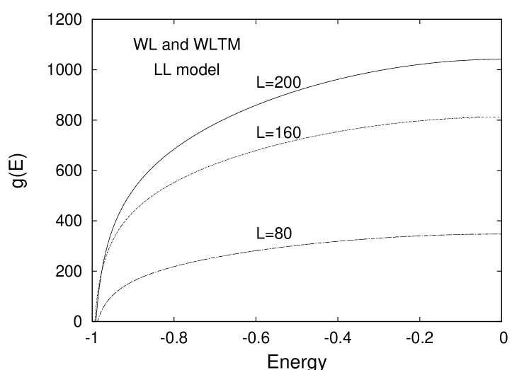
Figure 2: Plot of the logarithm of density of states, $g(E)$ against system energy per particle for 1-d LL model of lattice size $L=80$, $160$ and $220$ obtained using WL and WLTM algorithms.

Figure 3: The variation of orientational order parameter $(S)$ fo the 1-d LL model for different lattice sizes is plotted with temperature, obtained from both WL and WLTM algorithms.

Figure 4: The Susceptibility is shown as a function of temperature for the 1-d LL model of different lattice sizes. Data obtained from WL algorithm as well as from WLTM algorithm are plotted in this graph.

Figure 5: Variation of correlation function $\rho(r,T)$ with temperature for lattice size $L=80$ of 1-d LL model. $15$ different values of $r$ taken $2$, $4$, $6$, $8$, $10$, $12$, $14$, $16$, $18$, $20$, $22$, $24$, $26$, $28$ and $30$. The top most curve is for $r=2$ and the lower curves are for other values of $r$ given in the sequence above and in ascending order of $r$. The curves are the results obtained from the JDOS obtained using WL and WLTM algorithms. Comparison has been made with the exact results (the dots) obtained from romerio using equation 21 for $r=2$, $4$, $6$, $8$, $10$, $12$, $14$ and $16$.

Figure 6: Correlation function as a function of lattice spacing $r$ for seven different temperatures. Both WL and WLTM algorithms have been used. Comparison has been made with the exact results (the dots) of romerio obtained using equation 21.

Figure 7: Logarithm of density of states vs energy per particle for the 2-d XY model of sizes $5\times 5$, $10\times 10$, $15\times 15$ and $20\times 20$. The results obtained from both WL and WLTM algorithm are plotted.

Figure 8: The orientational order parameter is shown against temperature $T$ for 2-d XY model of different lattice sizes using both WL and WLTM algorithms.

Figure 9: The susceptibility of 2-d XY model for four liner lattice sizes $L=5$, $10$, $15$ and $20$ against temperature is plotted. All the data are from the results of two dimensional random walk in $E-S$ space using WL and WLTM algorithm. The height of the peak increases with the increase in system size. It is also noted that the position of peak shifts towards lower temperature with the increase of system size.

Figure 10: Variation of correlation function $\rho(r,T)$ with temperature for lattice size $L=20$ of the 2-d XY model. $10$ different values of $r$ taken $1$, $2$, $3$, $4$, $5$, $6$, $7$, $8$, $9$ and $10$. The top most curve is for $r=1$ and the lower curves are for other values of $r$ given in the sequence above and in ascending values of $r$. The curves are the results we obtained from joint density of states obtained using the both WL and WLTM algorithms.

Figure 11: Correlation function as a function of lattice spacing $r$ with eight different temperatures as parameter is plotted. Both the WL and WLTM algorithms were used.

V Results and discussion

V.1 The 1-d LL model:

In this model simulation was carried out for systems having linear dimension $L=80$, $160$ and $220$. The JDOS obtained by using the WLTM algorithm is shown in figure 1 as a function of energy and order parameter for $L=80$. In figure 2 we have plotted the DOS (actually its logarithm, $g(E)$) for the three lattices as a function of energy per particle obtained from the JDOS of figure 1 by using both WL and WLTM methods. From the knowledge of $g(E)$ one can calculate the average energy, specific heat etc. To determine the order parameter $S(T)$, one needs to perform 2d random walk in energy-order parameter space. Figure 3 shows the order parameter as a function of temperature for the 1d LL model for different lattice sizes obtained using WL and WLTM algorithms. From the figure it is clear that S decreases rapidly with temperature and with increase in system size. This is expected since the 1d LL model does not possess a true long range order at any finite temperature and the non-zero values of $S$ obtained is due to the finite size effect. Consequently the 1d LL model does not exhibit any finite temperature order-disorder phase transition. In figure 4, susceptibility is plotted against temperature for different system sizes. The peaks become sharp with the increase of system size. This also supports the absence of order-disorder phase transition.
The correlation function $\rho(r,T)$ has been plotted against temperature with $r$, the spacing between spins, in figure 5 for lattice size L=80 and 15 different values of $r$ ranging from $2$ to $30$. All data are obtained from 2-d random walk in $E-\rho$ space using both WL and WLTM algorithms. It may be noted that, we had to run one simulation for each value of $r$. With increase in temperature, the correlation between spins for a given value of $r$ decreases. Again $\rho(r,T)$ is plotted as a function of lattice spacing $r$ for seven different temperatures in figure 6. $\rho(r,T)$ decreases very rapidly with lattice spacing i.e. spins which are a large distance apart are uncorrelated. This is expected since in the thermodynamic limit, $\lim_{r\rightarrow\infty}\rho(r)=0$. The finite values of correlation function that appears in the figures is due to the finite size effect.

V.2 The 2-d XY model

In this model the simulation has been carried out for lattice sizes $5\times 5$, $10\times 10$, $15\times 15$ and $20\times 20$ using both WL and WLTM algorithms. Two dimensional random walk in two different spaces ($E-S$ and $E-\rho$) was performed to determine the order parameter, susceptibility and correlation function apart from average energy, specific heat etc which can be determined using 1-d random walk. The minimum energy for all lattice sizes was $3$. The upper limit of energies of these system sizes over which the simulation has been carried out were $50$, $200$, $450$ and $800$. We deleted a small region at the lower end of energy to overcome the trapping of the random walker. The order parameter (correlation function) can have values between $0$ and $1$ ($-0.5$ and $+0.5$). The whole energy and order parameter (correlation function) range is divided into a large number of bins of width $d_{e}=0.2$ and $d_{\phi}=0.01$ respectively.
In figure 7, the density of states obtained from the 2-d random walk for 2-d XY model for different lattice sizes have been plotted against the energy per particle. We have used both WL and WLTM algorithms to obtain the data presented in figure 7. The order parameter ($S(T)$) for 2-d XY model of linear lattice sizes $5$, $10$, $15$ and $20$ are plotted with temperature in figure 8. The system is known to possess no true long range order and a quasi-long-range-order disorder transition takes place due to unbinding of topological defects. Susceptibility of 2d XY model is also plotted as a function of temperature for four lattice sizes in figure 9. It is observed that the height of the susceptibility peak increases with the increase of system sizes and also the position of susceptibility peak is shifted towards the lower temperature with the increase of system size. In figure 10 we have plotted the correlation function $\rho(r,T)$ against temperature for ten values of $r$ for the XY-model. These were obtained from the JDOS computed by using WL and WLTM methods. The same data is depicted in a different way in figure 10, where we have plotted $\rho(r,T)$ against $r$ for eight different values of temperature.

VI Conclusion

We have presented the results of Monte Carlo simulation performed in the 1-d LL model and 2-d XY-model for the evaluation of joint density of states using the WL and WLTM algorithms. Agreement of the statistical averages of different quantities obtained by using the two algorithms is excellent. Calculation of JDOS for continuous spin models has been done earlier kisor . We have demonstrated in this work that, although computationally tedious, it is possible to use the WLTM method for the evaluation of the JDOS for a continuous spin model. This method may prove to be useful for future researchers who will need to generate the JDOS in a discrete or coninuous spin model.

VII Acknowledgment

We acknowledge the receipt of a research grant No. 03(1071)/06/EMR-II from Council of Scientific and Industrial Research (CSIR), India which helped us to procure the IBM x226 servers. One of the authors (SB) gratefully acknowledges CSIR, India, for the financial support.

References

- (1) P. M. C. de Oliveria, T. J. P. Penna and H. J. Hermann Braz. J. Phys. 26 (1996) 677; P. M. C. de Oliveria, Eur. Phys. J. B. 6 (1998) 111.
- (2) J. S. Wang and R. H. Swendsen, J. Stat. Phys. 106 (2001) 245.
- (3) F. Wang and D. P. Landau, Phys. Rev. Lett. 86 (2001) 2050; F. Wang and D. P. Landau, Phys. Rev. E 64 (2001) 056101.
- (4) M. S. Shell, P. G. Debenedetti and A. Z. Panagiotopoulos, J. Chem. Phys, 119 (2003) 9406.
- (5) R. G. Ghulghazaryan, S. Hayryan and C. Hu, J. Comput. Chem 28 (2007) 715.
- (6) M. S. Shell, P. G. Debenedetti and A. Z. Panagiotopoulos, Phys. Rev. E 66 (2002) 056703.
- (7) Q. Yan, R. Faller and J. J. de Pablo, J. Chem. Phys. 116 (2002) 8745.
- (8) D. P. Landau, S. Tsai and M. Exler, Am. J. Phys. 72 (2004) 1294.
- (9) J. Xu and H. Ma, Phys. Rev. E 75 (2007) 041115.
- (10) K. Mukhopadhyay, N. Ghoshal, S. K. Roy, Physics Letters A, 372 (2008) 3369.
- (11) S. Bhar and S. K. Roy, comp. Phys. Comm. 180 (2009) 699.
- (12) P. A. Lebwohl and G. Lasher, Phys. Rev. A 6 (1972) 426.
- (13) P. A. Vuillermot and M. V. Romerio, J. Phys. C 6 (1973) 2922; P. A. Vuillermot and M. V. Romerio, Commun. Math. Phys. 41 (1975) 281.
- (14) C. Zhou and R. N. Bhatt, Phys. Rev. E 72 (2005) 025701.
- (15) H. K. Lee, Y. Okabe and D. P. Landau, Compt. Phys. Commu., 175 (2006) 36.
- (16) M. Abramowitz and I. Stegun, A Handbook of Mathematical Functions, Dover, New York, 1970
- (17) E. Domany, M. Schick and R. H. Swendsen, Phys. Rev. Lett. 52 (1984) 1535.
- (18) J. M. Kosterlitz and D. J. Thouless, J. Phys. C: Solid State Phys, 6 (1973) 1181.
- (19) J. M. Kosterlitz, J. Phys. C: Solid State Phys., 7 (1974) 1046.
- (20) P. Olsson,Phys. Rev. B 52 (1995) 4511; P. Olsson, Phys. Rev. B 52 (1995) 4526; J. Maucourt and D. R. Grempel, Phys. Rev. B 56 (1997) 2572; P. Archambault, S. T. Bramwell et. al, J. Applied Phys. 83 (1998) 7234; G. Palma, T. Mayer and R. Labbe, Phys. Rev. E 66 (2002) 026108.
- (21) J. A. Nelder and R. Mead, Computer Journal, 7 (1965) 308; W. H. Press, S. A. Teukolsky et. al, Numerical Recipes in Fortran, Cambridge University press 1986.