Superconductivity between $H_{C_{2}}$ and $H_{C_{3}}$

Abstract.

Superconductivity for Type II superconductors in external magnetic fields of magnitude between the second and third critical fields is known to be restricted to a narrow boundary region. The profile of the superconducting order parameter in the Ginzburg-Landau model is expected to be governed by an effective one-dimensional model. This is known to be the case for external magnetic fields sufficiently close to the third critical field. In this text we prove such a result on a larger interval of validity.

1. Introduction

1.1. Background

When studying superconductivity in the Ginzburg-Landau model in strong magnetic fields, one encounters three critical values of the magnetic field strength. The first critical field is where a vortex appears and will not concern us in the present text. At the second critical field, denoted $H_{C_{2}}$, superconductivity becomes essentially restricted to the boundary and is weak in the interior. At the third critical field, $H_{C_{3}}$, superconductivity disappears altogether. In this paper we will discuss superconductivity in the zone between $H_{C_{2}}$ and $H_{C_{3}}$.

The Ginzburg-Landau model of superconductivity is the following functional,

$$\mathcal{E}[\psi,\mathbf{A}] =\int_{\Omega}|(\nabla-i\kappa H\mathbf{A})\psi|^{2}-\kappa^{2}|\psi|^{2}+\frac{\kappa^{2}}{2}|\psi|^{4}+(\kappa H)^{2}|{\rm curl}(\mathbf{A}-\mathbf{F})|^{2}\,dx\,.$$ (1.1)

Here $\psi\in W^{1,2}(\Omega)$ is a complex valued wave function, $\mathbf{A}\in W^{1,2}(\Omega,{\mathbb{R}}^{2})$ a vector potential, $\kappa$ the Ginzburg-Landau parameter (a material parameter), and $H$ is the strength of the applied magnetic field. The potential $\mathbf{F}:\Omega\to{\mathbb{R}}^{2}$ is the unique vector field satisfying,

$$\operatorname{curl}\mathbf{F}=1\,,\quad\operatorname{div}\mathbf{F}=0\quad\text{in}~{}\Omega\,,\qquad\qquad N\cdot\mathbf{F}=0\quad\text{on}~{}\partial\Omega\,,$$ (1.2)

where $N$ is the unit inward normal vector of $\partial\Omega$.

With this notation, the critical fields behave as follows for large $\kappa$:

$$H_{C_{2}}\approx\kappa+o(\kappa),\qquad H_{C_{3}}\approx\frac{\kappa}{\Theta_{0}}+o(\kappa),$$ (1.3)

where $\Theta_{0}\approx 0.59$ is a universal constant. The definition of $\Theta_{0}$ is recalled in (2.7) below.

Therefore, when we study the Ginzburg-Landau functional for $H=b\kappa$, $1<b<\Theta_{0}^{-1}$, superconductivity should be a boundary phenomenon. This was proved in a weak sense in [11].

Theorem 1.1 ([11]).

For any $b\in\left]1,\Theta_{0}^{-1}\right[$, there exists a constant $E_{b}$, such that, for $H=\kappa b$,

$$\inf_{(\psi,{\bf A})\in W^{1,2}(\Omega)\times W^{1,2}(\Omega;{\mathbb{R}}^{2})}{\mathcal{E}}_{\kappa,H}[\psi,{\bf A}]=-\sqrt{\kappa H}E_{b}|\partial\Omega|+o(\kappa),\qquad\text{ as }\kappa\rightarrow\infty.$$ (1.4)

Local energy results are also obtained in [11]. Theorem 1.1 indicates that superconductivity is uniformly distributed along the boundary. However, the constant $E_{b}$ is only defined as a limit and its calculation is not easy. A number of conjectures related to the calculation of $E_{b}$ are given in [11]. In [1] (see also [5, Chapter 14]), the constant $E_{b}$ is determined for $b$ in the vicinity of $\Theta_{0}^{-1}$. It turns out that the determination of the constant in this non-linear problem can be reduced to the positivity of a linear operator. Define the space ${\mathcal{B}}^{1}({\mathbb{R}}^{+})$ as

$${\mathcal{B}}^{1}({\mathbb{R}}^{+})=\{\phi\in L^{2}({\mathbb{R}}^{+})\,:\,\phi^{\prime}\in L^{2}({\mathbb{R}}^{+})\text{ and }t\phi\in L^{2}({\mathbb{R}}^{+})\}.$$ (1.5)

Define, for $z\in{\mathbb{R}}$, $\lambda>0$,

$${\mathcal{F}}_{z,\lambda}(\phi) :=\int_{0}^{+\infty}|\phi^{\prime}(t)|^{2}+(t-z)^{2}|\phi(t)|^{2}+\frac{\lambda}{2}|\phi(t)|^{4}-\lambda|\phi(t)|^{2}\,dt\,,$$ (1.6)

and let $f_{z,\lambda}$ be a non-negative minimizer of this functional (see Theorem 3.1 below for properties of minimizers—in particular the fact that $f_{z,\lambda}$ exists and is unique).

For given $\lambda>0$, minimize ${\mathcal{F}}_{z,\lambda}(f_{z,\lambda})$ over $z$ and denote a minimum by $\zeta(\lambda)$—we will prove below that such a minimum exists when $\lambda\in\left]\Theta_{0},1\right]$. By definition of $f_{\zeta(\lambda),\lambda}$,

$${\mathcal{F}}_{z,\lambda}(\phi)\geq{\mathcal{F}}_{\zeta(\lambda),\lambda}(f_{\zeta(\lambda),\lambda}),$$ (1.7)

for all $(z,\phi)\in{\mathbb{R}}\times{\mathcal{B}}^{1}({\mathbb{R}^{+}})$.

We also introduce a linear operator ${\mathfrak{k}}_{\lambda}$. Define, for $\nu\in{\mathbb{R}}$, $\lambda\in{\mathbb{R}^{+}}$, the operator ${\mathfrak{k}}_{\lambda}={\mathfrak{k}}_{\lambda}(\nu)$ to be the Neumann realization of

$${\mathfrak{k}}_{\lambda}(\nu)=-\frac{d^{2}}{dt^{2}}+(t-\nu)^{2}+\lambda f_{\zeta(\lambda),\lambda}(t)^{2},$$ (1.8)

on $L^{2}({\mathbb{R}}_{+})$. We denote by $\{\lambda_{j}(\nu)\}_{j=1}^{\infty}$ the spectrum of ${\mathfrak{k}}_{\lambda}(\nu)$. Also $\{v_{j}(t;\nu)\}_{j=1}^{\infty}$ will be the associated real, normalized eigenfunctions.

Remark 1.2.

Notice the following complication: Since we do not know that $\zeta(\lambda)$ is unique, the operator ${\mathfrak{k}}_{\lambda}(\nu)$ is really a family of operators,

$${\mathfrak{k}}^{(j)}_{\lambda}(\nu)=-\frac{d^{2}}{dt^{2}}+(t-\nu)^{2}+\lambda f_{\zeta_{j}(\lambda),\lambda}(t)^{2},$$

one for every minimum $\zeta_{j}(\lambda)$.

It follows from [1, 5] that

Theorem 1.3.

Let $\lambda\in\left]\Theta_{0},1\right[$. Suppose that there exists a minimum $\zeta(\lambda)$ such that for the corresponding choice of the operator ${\mathfrak{k}}_{\lambda}(\nu)$ we have

$$\lambda\leq\inf_{\nu\in\mathbb{R}}\lambda_{1}(\nu)\,.$$ (1.9)

Then

$$E_{\lambda^{-1}}=\frac{\lambda}{2}\|f_{\zeta(\lambda),\lambda}\|_{L^{4}({\mathbb{R}}^{+})}^{4}.$$ (1.10)

It is also proved in [1, 5] (see Proposition 14.2.13 in [5]) that there exists $\varepsilon>0$ such that (1.9) is satisfied for $\lambda\in\left]\Theta_{0},\Theta_{0}+\varepsilon\right[$. The objective of the present paper is to give explicit bounds on the magnitude of $\varepsilon$.

Remark 1.4.

A minimizer $f_{z,\lambda}$ of the functional ${\mathcal{F}}_{z,\lambda}$ will be a solution to the Euler-Lagrange equations for the minimization problem (1.6)

$$-u^{\prime\prime}+(t-z)^{2}u+\lambda|u|^{2}u=\lambda u,\qquad u^{\prime}(0)=0.$$ (1.11)

In particular, when $\nu=\zeta(\lambda)$ we have $\lambda_{1}(\nu)=\lambda$, since (by (1.11) with $z=\zeta(\lambda)$) $f_{\zeta(\lambda),\lambda}$ will be a positive eigenfunction of ${\mathfrak{k}}_{\lambda}(\zeta(\lambda))$.

1.2. Main results

We are not able to prove (1.9) for all $\lambda\in]\Theta_{0},1]$. Here we state some partial results. Clearly, $\nu=\zeta$ is a stationary point for $\lambda_{1}(\nu)$. Our first result shows that this is a local minimum.

Theorem 1.5.

1. Let $\Theta_{0}<\lambda\leq 1$. Then $\lambda_{1}(\nu)$ has a local minimum for $\nu=\zeta,$ i.e., there exist positive constants $\delta_{\lambda}$ and $c_{\lambda}$ such that for all $|\nu-\zeta|<\delta_{\lambda}$ it holds that

   $$\lambda_{1}(\nu)\geq\lambda+c_{\lambda}(\nu-\zeta)^{2}.$$

2. Let $\lambda>\Theta_{0},$ $z\in{\mathbb{R}},$ and let $f_{z,\lambda}$ be a positive minimizer of ${\mathcal{F}}_{z,\lambda}$. Define

   $$\lambda_{1}(\nu;z):=\inf\operatorname{Spec}\Big{\{}-\frac{d^{2}}{dt^{2}}+(t-\nu)^{2}+\lambda f_{z,\lambda}^{2}\Big{\}},$$ (1.12)

   where we consider the Neumann realization on $L^{2}({\mathbb{R}}^{+})$ of the operator.

   Then, $\lambda_{1}(\nu;z)\rightarrow 1$ as $\nu\rightarrow+\infty$. Furthermore, there exists $\nu_{0}=\nu_{0}(\lambda,z)>0$ such that

   $$\lambda_{1}(\nu;z)>1,$$ (1.13)

   for all $\nu\geq\nu_{0}$.

Remark 1.6.

In particular, the second item in Theorem 1.5 implies that (1.9) is not true for $\lambda>1$. It is therefore natural to expect that (1.9) will be valid if and only if $\lambda\in\left]\Theta_{0},1\right]$. Notice that we will not prove that a minimum $\zeta(\lambda)$ exists for $\lambda>1$. This explains the somewhat cumbersome statement in the second item in Theorem 1.5.

We also obtain an explicit range of values of $\lambda$ for which the condition (1.9) is satisfied. The results contain some explicit universal constants that will be defined later. In this introduction we will only state the numerical values obtained.

Theorem 1.7.

• Let $\Theta_{0}<\lambda\leq 1$. For all $\nu\leq 1.33$ it holds that $\lambda_{1}(\nu)\geq\lambda$.

• Let $\Theta_{0}\leq\lambda\leq 0.8$. Then (1.9) holds, i.e.

  $$\inf_{\nu\in\mathbb{R}}\lambda_{1}(\nu)\geq\lambda.$$

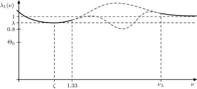
Figure 1.1. A schematic picture of what we know about $\lambda_{1}(\nu)$ from Theorems 1.5 and 1.7. The gray dashed parts show two possible scenarios.

In Section 2 we recall some well-known results about the linear de Gennes operator, and give some new spectral estimates. In Section 3 we study the nonlinear problem appearing from the functional $\mathcal{F}_{z,\lambda}(\phi)$ in (1.6) and prove (1.13). In Section 4 we consider the operator $\mathfrak{k}_{\lambda}(\nu)$ and prove the remainder of Theorem 1.5 and Theorem 1.7.

2. The linear problem

2.1. Reminder for the de Gennes operator

Define

$${\mathfrak{h}}(\xi)=-\frac{d^{2}}{dt^{2}}+(t-\xi)^{2},$$ (2.1)

in $L^{2}({\mathbb{R}}^{+})$ with Neumann boundary conditions at $0$. We will denote the eigenvalues of this operator by $\{\mu_{j}(\xi)\}_{j=1}^{\infty}$ and corresponding (real normalized) eigenfunctions by $u_{j}(t)=u_{j}(t;\xi)$.

From a similar calculation as the one leading to (A.18) in [2],

$$\mu_{1}(\xi)\geq 1-C_{1}\xi\exp(-\xi^{2}),$$ (2.2)

for some constant $C_{1}>0$ and for sufficiently large $\xi$. As part of the proof of Proposition 2.2 below we will obtain a weaker asymptotics of $\mu_{1}(\xi)$.

A basic identity from perturbation theory (Feynman-Hellmann) is

$$\mu_{j}^{\prime}(\xi)=-2\int_{0}^{+\infty}(t-\xi)|u_{j}(t;\xi)|^{2}\,dt.$$ (2.3)

An integration by parts, combined with the equation satisfied by $u_{j}(t;\xi)$ yields the useful alternative formula from Dauge-Helffer [3]:

$$\mu_{j}^{\prime}(\xi)=(\xi^{2}-\mu_{j}(\xi))|u_{j}(0;\xi)|^{2}\,.$$ (2.4)

From (2.4) it is simple to deduce that $\mu_{j}$ has a unique minimum attained at $\xi_{0}^{(j)}$ satisfying

$$\mu_{j}(\xi_{0}^{(j)})=(\xi_{0}^{(j)})^{2}\,.$$ (2.5)

Notice that, from (2.3), we obtain

$$\xi_{0}^{(j)}>0\,,$$ (2.6)

for all $j$. We will sometimes write $\xi_{0}=\xi_{0}^{(1)}$. By definition

$$\Theta_{0}=\inf_{\xi\in\mathbb{R}}\mu_{1}(\xi)=\mu_{1}(\xi_{0}^{(1)})=(\xi_{0}^{(1)})^{2}.$$ (2.7)

Finally, we recall that

$$\mu_{j}(0)=1+4(j-1)\,,\quad\lambda_{j}^{D}(0)=3+4(j-1)\,,$$ (2.8)

where $\lambda_{j}^{D}(\xi)$ denotes the $j$-th eigenvalue of the Dirichlet realization of $\mathfrak{h}(\xi)$ in $L^{2}(\mathbb{R}^{+})$. These identities follow upon noticing that the eigenfunctions of the harmonic oscillator on the entire line are respectively even or odd functions.

2.2. Comparison Dirichlet-Neumann

In this section we recall useful links between the Dirichlet spectrum and the Neumann spectrum of the family $\mathfrak{h}(\xi)$ ($\xi\in\mathbb{R}$) in $L^{2}(\mathbb{R}^{+})$ . By domain monotonicity, it is standard that $\xi\mapsto\lambda_{j}^{D}(\xi)$ is monotonically decreasing. By comparison of the form domains:

$$\mu_{j}(\xi)\leq\lambda_{j}^{D}(\xi)\,.$$ (2.9)

Also,

$$\lim_{\xi\to+\infty}\lambda_{1}^{D}(\xi)=\lim_{\xi\to+\infty}\mu_{1}(\xi)=1\,,$$

$$\lim_{\xi\to+\infty}\lambda_{2}^{D}(\xi)=\lim_{\xi\to+\infty}\mu_{2}(\xi)=3\,.$$

Using Sturm-Liouville theory, we also observe that, for any $j\geq 2$ and any $\xi$, there exists $\xi^{\prime}$ such that

$$\mu_{j}(\xi)=\lambda_{j-1}^{D}(\xi^{\prime})\,.$$ (2.10)

In particular, using that

$$\inf_{\xi\in\mathbb{R}}\lambda_{1}^{D}(\xi)=1\,,$$ (2.11)

we get

$$\mu_{2}(\xi)>1\,.$$ (2.12)

2.3. The virial theorem

For $\ell>0$, the map $t\mapsto\ell t$ can be unitarily implemented on $L^{2}(\mathbb{R}^{+})$ by the operator $Uf(t)=\sqrt{\ell}f(\ell t)$. Therefore, $\mathfrak{h}(\xi)$ is isospectral to the (Neumann realization of the) operator

$${\mathfrak{k}}_{\ell}:=-\ell^{-2}\frac{d^{2}}{dt^{2}}+(\ell t-\xi)^{2}.$$

Since the eigenvalues are unchanged when $\ell$ varies we can take the derivative at $\ell=1$ and find (using (2.3))

$$0 =\int_{0}^{+\infty}|u_{j}^{\prime}(t;\xi)|^{2}\,dt-\int_{0}^{+\infty}t(t-\xi)|u_{j}(t;\xi)|^{2}\,dt$$

$$=\int_{0}^{+\infty}|u_{j}^{\prime}(t;\xi)|^{2}\,dt-\int_{0}^{+\infty}(t-\xi)^{2}|u_{j}(t;\xi)|^{2}\,dt+\frac{\xi}{2}\mu_{j}^{\prime}(\xi).$$

Combined with the definition of the energy

$$\mu_{j}(\xi)=\int_{0}^{+\infty}|u_{j}^{\prime}(t;\xi)|^{2}\,dt+\int_{0}^{+\infty}(t-\xi)^{2}|u_{j}(t;\xi)|^{2}\,dt\,,$$

we get

$$\int_{0}^{+\infty}|u_{j}^{\prime}(t;\xi)|^{2}\,dt =\frac{\mu_{j}(\xi)}{2}-\frac{\xi\mu_{j}^{\prime}(\xi)}{4}\,,$$ (2.13)

and

$$\int_{0}^{+\infty}(t-\xi)^{2}|u_{j}(t;\xi)|^{2}\,dt =\frac{\mu_{j}(\xi)}{2}+\frac{\xi\mu_{j}^{\prime}(\xi)}{4}\,.$$ (2.14)

2.4. Lower bounds on $\mu_{j}(\xi)$

2.4.1. Estimates on $\mu_{1}$

As a warm-up, we recall the lower bound on $\mu_{1}(\xi)$. Let $u_{1}(\,\cdot\,;\xi)$ be the ground state of ${\mathfrak{h}}(\xi)$. We use this function as a trial state for ${\mathfrak{h}}(0)$ and find

$$1=\inf{\rm Spec}\,{\mathfrak{h}}(0) <\langle u_{1}(\,\cdot\,;\xi),{\mathfrak{h}}(0)u_{1}(\,\cdot\,;\xi)\rangle=\mu_{1}(\xi)+2\xi\int_{0}^{+\infty}(t-\xi)u_{1}(t;\xi)^{2}\,dt+\xi^{2}.$$

So we obtain the inequality :

$$1<\mu_{1}(\xi)-\xi\mu_{1}^{\prime}(\xi)+\xi^{2}\,.$$ (2.15)

We insert $\xi_{0}^{(1)}$, using $(\xi_{0}^{(1)})^{2}=\Theta_{0}=\min_{\xi}\mu_{1}(\xi)$, $\mu_{1}^{\prime}(\xi_{0}^{(1)})=0$ and get

$$\frac{1}{2}<\Theta_{0}\,.$$ (2.16)

2.4.2. Estimates on $\mu_{j}$, $j>1$

From (2.5), (2.6) and the fact that $\lim_{\xi\to+\infty}\mu_{j}(\xi)=(2j-1)$ we find that

$$0<\xi^{(j)}_{0}<\sqrt{2j-1}.$$

The function $\xi\mapsto\mu_{j}(\xi)$ decreases from its value $\mu_{j}(0)=4j-3$ until it arrives at its minimum at $\xi^{(j)}_{0}$, after which it becomes increasing, so there exists a unique point $\widehat{\xi}_{j}>0$ such that $\mu_{j}(\widehat{\xi}_{j})=2j-1$. By comparison with the harmonic oscillator on a half axis it can be seen that $\widehat{\xi}_{j}$ coincides with the smallest value of $\xi$ for which $h_{j}^{\prime}(\xi)=0$, where $h_{j}^{\prime}(\xi)$ denotes the $j$th Hermite function. In particular one easily finds that

$$\widehat{\xi}_{2}=1,\quad\text{and}\quad\widehat{\xi}_{3}=\sqrt{5/2}.$$ (2.17)

To get the behavior of $\widehat{\xi}_{j}$ as $j\to\infty$ we observe by reflection that $-\widehat{\xi}_{j}$ is given by the value of $\xi$ for which $\mu_{1}(\xi)=2j-1$.

Let us get an upper bound on $\mu_{1}(\xi)$ for $\xi$ negative. For any $\gamma>0$ and any $\xi\in\mathbb{R}$ we use the inequality

$$(t-\xi)^{2}\leq(1+\gamma)t^{2}+(1+1/\gamma)\xi^{2}$$

to obtain the quadratic form comparison (here and below $\int_{0}^{+\infty}|u|^{2}\,dt=1$)

$$\int_{0}^{+\infty}|u^{\prime}|^{2}+(t-\xi)^{2}|u|^{2}\,dt\leq\int_{0}^{+\infty}|u^{\prime}|^{2}+(1+\gamma)t^{2}|u|^{2}\,dt+(1+1/\gamma)\xi^{2}.$$

Comparing the first eigenvalue $\mu(\xi)$ with the first eigenvalue of the (scaled) harmonic oscillator, we find

$$\mu_{1}(\xi)\leq\sqrt{1+\gamma}+(1+1/\gamma)\xi^{2}.$$

The upper bound we get from this seems to be poor.

For any $\gamma>0$ and any $\xi\in\mathbb{R}$ we use the inequality

$$(t-\widehat{\xi}_{j})^{2}\leq(1+\gamma)(t-\xi)^{2}+(1+1/\gamma)(\widehat{\xi}_{j}-\xi)^{2}$$

to obtain the quadratic form comparison

$$\int_{0}^{+\infty}|u^{\prime}|^{2}+(t-\widehat{\xi}_{j})^{2}|u|^{2}\,dt\leq\int_{0}^{+\infty}|u^{\prime}|^{2}+(1+\gamma)(t-\xi)^{2}|u|^{2}\,dt+(1+1/\gamma)(\widehat{\xi}_{j}-\xi)^{2}.$$

By scaling and change of function, we have that the quadratic form on the right-hand side is unitary equivalent to

$$\sqrt{1+\gamma}\int_{0}^{+\infty}|u^{\prime}|^{2}+(t-(1+\gamma)^{1/4}\xi)^{2}|u|^{2}\,dt+(1+1/\gamma)(\widehat{\xi}_{j}-\xi)^{2}.$$

In particular, with the choice $\xi=\xi^{(j)}_{0}(1+\gamma)^{-1/4}$ we obtain, comparing the $j$th eigenvalue of the corresponding operators and using (2.5), that

$$2j-1=\mu_{j}(\widehat{\xi}_{j}) \leq\sqrt{1+\gamma}\mu_{j}(\xi^{(j)}_{0})+(1+1/\gamma)\bigl{(}\widehat{\xi}_{j}-\xi^{(j)}_{0}(1+\gamma)^{-1/4}\bigr{)}^{2}$$

$$=\sqrt{1+\gamma}\bigl{(}\xi^{(j)}_{0}\bigr{)}^{2}+(1+1/\gamma)\bigl{(}\widehat{\xi}_{j}-\xi^{(j)}_{0}(1+\gamma)^{-1/4}\bigr{)}^{2}.$$

Now let $j=2$. By (2.17) we have

$$3\leq\sqrt{1+\gamma}\bigl{(}\xi^{(2)}_{0}\bigr{)}^{2}+(1+1/\gamma)\bigl{(}\xi^{(2)}_{0}(1+\gamma)^{-1/4}-1\bigr{)}^{2}.$$

Completing the square, we get

$$\bigl{(}\xi^{(2)}_{0}-(1+\gamma)^{-3/4}\bigr{)}^{2}\geq\frac{2\gamma}{(1+\gamma)^{3/2}},$$

and hence the inequality

$$\xi^{(2)}_{0}>\frac{1+\sqrt{2\gamma}}{(1+\gamma)^{3/4}}$$ (2.18)

(since $\frac{1-\sqrt{2\gamma}}{(1+\gamma)^{3/4}}<1$ for all $\gamma>0$. Indeed, the function $\gamma\mapsto\frac{1-\sqrt{2\gamma}}{(1+\gamma)^{3/4}}$ starts at $1$ for $\gamma=0$ and then decreases to its minimal value $-1/\sqrt{3}$ for $\gamma=8$ after which it increases to $0$ as $\gamma\to\infty$). Optimizing (2.18) in $\gamma>0$ we find that the maximal value is attained for $\gamma=1/2$, for which we have

$$\xi^{(2)}_{0}>\frac{2^{7/4}}{3^{3/4}}\approx 1.48.$$

The corresponding lower bound for $\mu_{2}$ is

$$\mu_{2}\bigl{(}\xi^{(2)}_{0}\bigr{)}\geq\frac{2^{7/2}}{3^{3/2}}\approx 2.18.$$ (2.19)

Continuing with $j=3$, we arrive at the inequality

$$5\leq\sqrt{1+\gamma}\bigl{(}\xi^{(3)}_{0}\bigr{)}^{2}+(1+1/\gamma)\bigl{(}\xi^{(3)}_{0}(1+\gamma)^{-1/4}-\sqrt{5/2}\bigr{)}^{2}.$$

The same type of calculation shows that

$$\xi^{(3)}_{0}>\sqrt{\frac{5}{2}}\frac{1+\sqrt{\gamma}}{(1+\gamma)^{3/4}}.$$

Optimizing over $\gamma>0$ yields $\gamma=\frac{1}{2}\bigl{(}13-3\sqrt{17}\bigr{)}\approx 0.32$ with corresponding inequality

$$\xi^{(3)}_{0}>\frac{\sqrt{5}\Bigl{(}2+\sqrt{26-6\sqrt{17}}\Bigr{)}}{(30-6\sqrt{17})^{3/4}}\approx 2.01$$

which in turn gives

$$\mu_{3}(\xi^{(3)}_{0})\geq\frac{5\Bigl{(}2+\sqrt{26-6\sqrt{17}}\Bigr{)}^{2}}{(30-6\sqrt{17})^{3/2}}\approx 4.04.$$

Remark 2.1.

We can compare these estimates with the numerical values

$$\xi^{(2)}_{0}\approx 1.62,\quad\mu_{2}(\xi^{(2)}_{0})\approx 2.64,\quad\xi^{(3)}_{0}\approx 2.16,\quad\text{and}\quad\mu_{3}(\xi^{(3)}_{0})\approx 4.65.$$

2.5. Asymptotics of $u_{1}$

We end this section by giving an asymptotic formula for $u_{1}(\,\cdot\,;\xi)$ for large $\xi$.

Proposition 2.2.

For all $\alpha<1$ there exist $C_{\alpha}>0$ and $\Xi_{0}>0$ such that

$$\Bigl{|}u_{1}(t,\xi)-\frac{1}{\sqrt{\pi}}\exp\bigl{[}-(t-\xi)^{2}/2\bigr{]}\Bigr{|}\leq C_{\alpha}\exp(-\alpha\xi^{2}/2),$$ (2.20)

for all $t\in{\mathbb{R}}^{+}$ and all $\xi>\Xi_{0}$.

Proof.

Let $\phi$ be smooth, $\phi(t)=0$ for $t\leq 1$, $\phi(t)=1$ for $t\geq 2$ and define

$$\tilde{u}(t)=\phi(t)\frac{1}{\sqrt{\pi}}\exp\big{[}-(t-\xi)^{2}/2\big{]}.$$ (2.21)

An elementary calculation now yields (for $\xi>2$ and some constant $C>0$)

$$\bigl{\|}[{\mathfrak{h}}(\xi)-1]\tilde{u}\bigr{\|}^{2}\leq C\xi^{2}\exp\bigl{(}-(\xi-2)^{2}\bigr{)},$$ (2.22)

Using the lower bound on $\mu_{2}(\xi)$ and the spectral theorem this implies that

$$|\mu_{1}(\xi)-1|\leq C\exp(-\alpha\xi^{2}/2),$$ (2.23)

and the existence of a (possibly non-normalized) ground state eigenfunction $u_{1}$ such that

$$\|\tilde{u}-u_{1}\|_{2}\leq C\exp(-\alpha\xi^{2}/2).$$ (2.24)

One now obtains the similar estimate in $W^{1,2}(\mathbb{R}^{+})$, from which the pointwise estimate follows. ∎

3. Estimates on the non-linear problem

We now analyse the functional ${\mathcal{F}}_{z,\lambda}$ defined in (1.6).

3.1. Preliminaries

We introduce the notation

$${\mathfrak{I}}(\lambda):=\{\xi\in{\mathbb{R}}\,:\,\mu_{1}(\xi)<\lambda\}.$$ (3.1)

For future reference, we notice that if $\Theta_{0}<\lambda<1$, then there exist $\xi_{1}(\lambda),\xi_{2}(\lambda)>0$ such that

$${\mathfrak{I}}(\lambda)=\bigl{]}\xi_{1}(\lambda),\xi_{2}(\lambda)\bigr{[}.$$ (3.2)

For $\lambda=1$ we have ${\mathfrak{I}}(\lambda)=\left[0,\infty\right[$.

Theorem 3.1.

• For all $z\in{\mathbb{R}},\lambda>0,$ the functional ${\mathcal{F}}_{z,\lambda}$ admits a non-negative minimizer $f_{z,\lambda}\in{\mathcal{B}}^{1}({\mathbb{R}}^{+})$, which is non-trivial if and only if $\lambda>\mu_{1}(z)$. The minimizer $f_{z,\lambda}$ is a solution to the Euler-Lagrange equation (1.11) and satisfies the bound

  $$\|f_{z,\lambda}\|_{\infty}\leq 1\,.$$ (3.3)

  Furthermore, minimizers are unique up to multiplication by a constant $c\in{\mathbb{S}}^{1}\subset{\mathbb{C}}$.

• For all $\varepsilon\in\left]0,1/2\right[$, $\lambda>0$ and $z\in{\mathfrak{I}}(\lambda)$, there exist constants $c_{\varepsilon},C_{\varepsilon}>0$ such that

  $$c_{\varepsilon}\exp\Big{(}-\Big{[}\frac{1}{2}+\varepsilon\Big{]}(t-z)^{2}\Big{)}\leq f_{z,\lambda}(t)\leq C_{\varepsilon}\exp\Big{(}-\Big{[}\frac{1}{2}-\varepsilon\Big{]}(t-z)^{2}\Big{)}.$$ (3.4)

Proof.

The first item in Theorem 3.1 is a slight improvement of known results (see [5, Proposition 14.2.1 and 14.2.2]), so we will only give brief indications of proof. For given $z$ and $\lambda$ the functional is clearly bounded from below, so the existence of minimizers is standard. Also, by differentiation of the absolute value, we see that minimizers can be chosen non-negative. The proof of the non-triviality statement is also straight-forward. The equation (1.11) follows by variation around a minimum, and (3.3) is a consequence of the maximum principle applied to (1.11).

We finally consider the uniqueness question. Let $u$ be a minimizer and let $f=|u|$. By the Euler-Lagrange equation (1.11) we see that

$${\mathfrak{k}}_{\lambda}(z)f=\lambda f,\qquad{\mathfrak{k}}_{\lambda}(z)u=\lambda u.$$ (3.5)

By Cauchy uniqueness, we therefore have $u=cf$ for some $c\in{\mathbb{S}}^{1}$. Therefore, to prove uniqueness it suffices to prove uniqueness of non-negative minimizers. The proof of this (which does not use any bound on the value of $\lambda$) is given in the proof of [5, Proposition 14.2.2] and will not be repeated.

The upper and lower bounds in (3.4) can both be proved using the following strategy, so we only consider the upper bound. We start from the equation for $f_{z,\lambda}$ in the form

$$f_{z,\lambda}^{\prime\prime}(t)=[(t-z)^{2}+\lambda f_{z,\lambda}^{2}(t)-\lambda]f_{z,\lambda}(t).$$ (3.6)

Define, for $\alpha<1$, the function $g$ as $g(t)=C\exp(-\frac{\alpha}{2}(t-z)^{2})$, for some constant $C>0$. Then

$$g^{\prime\prime}(t)=[\alpha^{2}(t-z)^{2}-\alpha]g(t).$$ (3.7)

Choose $T>z$ so large that

$$0<[\alpha^{2}(t-z)^{2}-\alpha]\leq[(t-z)^{2}+\lambda f_{z,\lambda}^{2}(t)-\lambda],$$ (3.8)

for all $t\geq T$. This is possible since $\alpha<1$. Choose $C>0$ in such a way that

$$g(T)>f_{z,\lambda}(T).$$ (3.9)

Suppose that the inequality $g(t)\geq f_{z,\lambda}(t)$ fails for some $t>T$. Since both functions tend to $0$ at $+\infty$ (at least along some sequence, since $f\in L^{2}({\mathbb{R}}^{+})$), we deduce that $u:=f-g$ has a positive maximum at some point $t_{0}>T$. Thus $u^{\prime\prime}(t_{0})\leq 0$. But, for $t\geq T$, we have

$$u^{\prime\prime}(t) =[(t-z)^{2}+\lambda f_{z,\lambda}^{2}(t)-\lambda]f_{z,\lambda}(t)-[\alpha^{2}(t-z)^{2}-\alpha]g(t)$$

$$\geq[\alpha^{2}(t-z)^{2}-\alpha]u(t).$$ (3.10)

At $t_{0}$ this is strictly positive and we get a contradiction. ∎

By a continuity argument, we find

Proposition 3.2.

For $0<\lambda\leq 1$, the function

$${\mathbb{R}}\ni z\mapsto{\mathcal{F}}_{z,\lambda}(f_{z,\lambda})$$ (3.11)

admits a minimum $\zeta(\lambda)>0$.

Notice that for $\lambda>1$, the existence of a minimum is an open problem.

Proof.

Only the case $\lambda=1$ needs some consideration. We will prove that the minimal energy in that case tends to $0$ as $z\to+\infty$. By continuity this implies the proposition. We calculate, for arbitrary $\phi\in{\mathcal{B}}^{1}({\mathbb{R}}^{+})$ and $\alpha\in\left]0,1\right[$, and estimating (part of) the quadratic expression from below by the linear ground state energy

$${\mathcal{F}}_{z,1}(\phi) \geq\int_{0}^{+\infty}\bigl{[}\alpha(t-z)^{2}+(1-\alpha)\mu_{1}(z)-1\bigr{]}|\phi|^{2}+\frac{1}{2}|\phi|^{4}\,dt$$

$$\geq\int_{\bigl{\{}|t-z|\leq\sqrt{[1-(1-\alpha)\mu_{1}(z)]/\alpha}\bigr{\}}}\bigl{[}(1-\alpha)\mu_{1}(z)-1\bigr{]}|\phi|^{2}+\frac{1}{2}|\phi|^{4}\,dt$$

$$\geq-\bigl{[}(1-\alpha)\mu_{1}(z)-1\bigr{]}^{2}\sqrt{\frac{1-(1-\alpha)\mu_{1}(z)}{\alpha}}$$

$$=-\bigl{[}1-\mu_{1}(z)+\alpha\mu_{1}(z)\bigr{]}^{2}\sqrt{\frac{1-\mu_{1}(z)+\alpha\mu_{1}(z)}{\alpha}},$$ (3.12)

where the last inequality follows by completing the square. We choose $\alpha=\alpha(z)=1-\mu_{1}(z)\rightarrow 0$ as $z\rightarrow+\infty$ to get the conclusion. ∎

We can now prove (1.13).

Proof of the second item in Theorem 1.5.

Let $z\in{\mathbb{R}}$ and let $f_{z,\lambda}$ be a positive minimizer of ${\mathcal{F}}_{z,\lambda}$. Notice that $z$ and $\lambda$ will be fixed in the remainder of the proof. We therefore write $f$ instead of $f_{z,\lambda}$. We also denote by $\tilde{\lambda}_{j}(\nu)=\lambda_{j}(\nu,z)$ the eigenvalues of the operator in (1.12).

We apply Temple’s inequality (see [10]) with $u_{1}:=u_{1}(\,\cdot\,;\nu)$ as a test function. Under the condition that $\tilde{\lambda}_{2}(\nu)>A$, Temple’s inequality says that

$$\tilde{\lambda}_{1}(\nu)\geq A-\frac{B}{\tilde{\lambda}_{2}(\nu)-A},$$ (3.13)

where

$$A=\Big{\langle}u_{1},\Big{\{}-\frac{d^{2}}{dt^{2}}+(t-\nu)^{2}+\lambda f^{2}\Big{\}}u_{1}\Big{\rangle}=\mu_{1}(\nu)+\lambda\|fu_{1}\|_{2}^{2}$$

and

$$B=\Big{\|}\Big{\{}-\frac{d^{2}}{dt^{2}}+(t-\nu)^{2}+\lambda f^{2}\Big{\}}u_{1}\Big{\|}_{2}^{2}-A^{2}=\lambda^{2}\|f^{2}u_{1}\|_{2}^{2}-\lambda^{2}\|fu_{1}\|_{2}^{4}.$$

Using the upper bound in (2.20) and (3.4), $\|fu_{1}\|_{2}\rightarrow 0$ as $\nu\rightarrow\infty$. Since $\tilde{\lambda}_{2}(\nu)\geq\mu_{2}(\nu)$ we see that the condition $\tilde{\lambda}_{2}(\nu)>A$ is satisfied for large $\nu$’s, and there

$$\tilde{\lambda}_{1}(\nu)\geq\mu_{1}(\nu)+\lambda\|fu_{1}\|_{2}^{2}-C\lambda^{2}\|f^{2}u_{1}\|_{2}^{2},$$ (3.14)

for some $C>0$ independent of $\nu$.

Using the upper bounds in (2.20) and (3.4), we get for all $0<\alpha<1$, and large $\nu$,

$$\|f^{2}u_{1}\|_{2}^{2} \leq C\exp(-\alpha\nu^{2})+C\int_{-\infty}^{+\infty}\exp(-2\alpha(t-z)^{2})\exp(-\alpha(t-\nu)^{2})\,dt$$

$$\leq C\exp(-\alpha\nu^{2})+C^{\prime}\exp(-2\alpha^{\prime}\nu^{2}/3),$$ (3.15)

where $\alpha^{\prime}<\alpha$ is arbitrary.

Without striving for optimality, we make the simple estimate

$$\|fu_{1}\|_{2}^{2}\geq\int_{\nu/2-1}^{\nu/2+1}f^{2}u_{1}^{2}\,dt.$$ (3.16)

In this interval of integration it follows from (2.20) that $u_{1}^{2}\geq C\exp\bigl{(}-(\nu/2+1)^{2}\bigr{)}$ and from (3.4) that $f^{2}\geq C\exp(-\beta\nu^{2}/4)$ for any $\beta>1$. Inserting in the integral yields, for any $\beta^{\prime}>1$,

$$\|fu_{1}\|_{2}^{2}\geq C\exp(-\beta^{\prime}\nu^{2}/2).$$ (3.17)

Combining (3.14), (3.1), (3.17) and the asymptotics of $\mu_{1}$ from (2.2) gives that

$$\tilde{\lambda}_{1}(\nu)>1,$$ (3.18)

for large $\nu$, which is (1.13).

To prove that $\tilde{\lambda}_{1}(\nu)\rightarrow 1$, we use the variational principle with $u_{1}=u_{1}(\,\cdot\,;\nu)$ as a test function. Notice that by the lower bound just established, we only need to prove an upper bound with limit $1$ at infinity. The variational principle gives

$$\tilde{\lambda}_{1}(\nu)\leq\mu_{1}(\nu)+\lambda\|fu_{1}\|_{2}^{2}.$$ (3.19)

Since we have seen above that $\|fu_{1}\|_{2}\rightarrow 0$ and $\mu_{1}(\nu)\rightarrow 1$ in the large $\nu$ limit, this implies the upper bound required. ∎

3.2. A virial-type result

The function $f_{\zeta,\lambda}$ satisfies the Euler-Lagrange equation (1.11). Since, $\zeta=\zeta(\lambda)$ is a minimum for the non-linear energy, we get

$$\int_{0}^{+\infty}(t-\zeta)f_{\zeta,\lambda}^{2}\,dt=0.$$ (3.20)

In particular it holds that $\zeta(\lambda)>0$.

Moreover, multiplying (1.11) by $f_{\zeta,\lambda}$ and integrating, we obtain

$$\|f_{\zeta,\lambda}^{\prime}\|_{2}^{2}+\|(t-\zeta)f_{\zeta,\lambda}\|_{2}^{2}+\lambda\|f_{\zeta,\lambda}\|_{4}^{4}=\lambda\|f_{\zeta,\lambda}\|_{2}^{2}\,.$$ (3.21)

Lemma 3.3.

Assume that $\Theta_{0}\leq\lambda\leq 1$ and that $(\zeta,f_{\zeta,\lambda})$ is a minimizer of the functional (1.6). Then

$$\|f^{\prime}_{\zeta(\lambda),\lambda}\|_{2}^{2}-\|(t-\zeta(\lambda))f_{\zeta(\lambda),\lambda}\|_{2}^{2}+\frac{\lambda}{4}\|f_{\zeta(\lambda),\lambda}\|_{4}^{4} =0\,,$$ (3.22)

$$2\|f^{\prime}_{\zeta(\lambda),\lambda}\|_{2}^{2}+\frac{5\lambda}{4}\|f_{\zeta(\lambda),\lambda}\|_{4}^{4} =\lambda\|f_{\zeta(\lambda),\lambda}\|_{2}^{2}\,,$$ (3.23)

and

$$2\|(t-\zeta(\lambda))f_{\zeta(\lambda),\lambda}\|_{2}^{2}+\frac{3\lambda}{4}\|f_{\zeta(\lambda),\lambda}\|_{4}^{4} =\lambda\|f_{\zeta(\lambda),\lambda}\|_{2}^{2}\,.$$ (3.24)

Proof.

By a change of variable and of function in the functional ${\mathcal{F}}_{z,\lambda}$ we get a rescaled functional

$$\phi\mapsto\int_{0}^{+\infty}\rho^{2}|\phi^{\prime}(t)|^{2}+\Bigl{(}\frac{t}{\rho}-\zeta\Bigr{)}^{2}|\phi(t)|^{2}+\frac{\lambda\rho}{2}|\phi(t)|^{4}-\lambda|\phi(t)|^{2}\,dt$$

with same infimum. Expressing that the infimum is independent of $\rho$, we obtain (using (3.20)) at $\rho=1$ and $\zeta=\zeta(\lambda)$, the identity (3.22). Combining with (3.21) we also get (3.23) and (3.24). ∎

3.3. Different bounds on $f_{\zeta,\lambda}$

Proposition 3.4.

Assume that $\Theta_{0}\leq\lambda\leq 1$ and let $(\zeta,f_{\zeta,\lambda})$ be a minimum of the function $(z,f)\mapsto{\mathcal{F}}_{z,\lambda}(f)$ with ${\mathcal{F}}$ defined in (1.6). Then

$$f_{\zeta,\lambda}(0)^{2}=\frac{2}{\lambda}\bigl{(}\lambda-\zeta^{2}\bigr{)}.$$ (3.25)

Furthermore,

$$2(\lambda-\zeta^{2})\leq\lambda\|f_{\zeta,\lambda}\|_{\infty}^{2}\leq\frac{9}{2^{4/3}}\zeta^{2/3}\lambda^{1/3}\biggl{(}\frac{1}{2}-\frac{5(\lambda-\Theta_{0})}{12\zeta^{1/2}\lambda\|u_{1}(\,\cdot\,;\xi_{0})\|_{4}^{2}}\biggr{)}^{1/3}(\lambda-\mu_{1}(\zeta))$$ (3.26)

and

$$\frac{\lambda-\Theta_{0}}{\|u_{1}(\,\cdot\,:\xi_{0})\|_{4}^{2}}\leq\lambda\|f_{\zeta,\lambda}\|_{4}^{2}\leq\frac{3}{2}\zeta^{1/2}(\lambda-\mu_{1}(\zeta)).$$ (3.27)

Remark 3.5.

A numerical calculation yields the approximate value $\|u_{1}(\,\cdot\,;\xi_{0})\|_{4}^{4}\approx 0.584$. One can also get a lower bound to $\|u_{1}(\,\cdot\,;\xi_{0})\|_{4}^{4}$ using (3.27): We have

$$\|u_{1}(\,\cdot\,;\xi_{0})\|_{4}^{4}\geq\frac{4}{9}\lim_{\lambda\rightarrow\Theta_{0}}\frac{(\lambda-\Theta_{0})^{2}}{\zeta(\lambda)\bigl{(}\lambda-\mu_{1}(\zeta(\lambda))\bigr{)}^{2}}=\frac{4}{9\xi_{0}}\approx 0.579.$$

Proof.

The lower bound in (3.26) is an easy consequence of (3.25). Both are proved in [11]. We reproduce the short proof for the sake of completeness. Indeed, define the function

$$H(t)=f_{\zeta,\lambda}^{\prime}(t)^{2}-(t-\zeta)^{2}f_{\zeta,\lambda}(t)^{2}+\lambda f_{\zeta,\lambda}(t)^{2}-\frac{\lambda}{2}f_{\zeta,\lambda}(t)^{4}.$$

A calculation, using (1.11) shows that $H^{\prime}(t)=-2(t-\zeta)f_{\zeta,\lambda}(t)^{2}$. By exponential decay it also holds that $\lim_{t\to\infty}H(t)=0$. Hence, by (3.20) we have that $H(0)=-\int_{0}^{\infty}H^{\prime}(t)\,dt=0$. On the other hand we also have $H(0)=(\lambda-\zeta^{2})f_{\zeta,\lambda}(0)^{2}-\frac{\lambda}{2}f_{\zeta,\lambda}(0)^{4}$. Since $f_{\zeta,\lambda}(0)\neq 0$, we get the equality in (3.25).

We continue with the lower bound in (3.27). By definition we have

$$-\frac{\lambda}{2}\|f_{\zeta,\lambda}\|_{4}^{4}={\mathcal{F}}_{\zeta,\lambda}[f_{\zeta,\lambda}]=\inf_{z\in{\mathbb{R}},\phi\in B^{1}}{\mathcal{F}}_{z,\lambda}[\phi].$$ (3.28)

We insert the trial state $z=\xi_{0}$, $\phi=\rho u_{1}(\,\cdot\,;\xi_{0})$, with $\rho=\sqrt{(\lambda-\Theta_{0})/[\lambda\|u_{1}(\,\cdot\,;\xi_{0})\|_{4}^{4}]}$, in (3.28). This yields,

$$-\frac{\lambda}{2}\|f_{\zeta,\lambda}\|_{4}^{4}\leq-\frac{\lambda}{2}\frac{(\lambda-\Theta_{0})^{2}}{\lambda^{2}\|u_{1}(\,\cdot\,;\xi_{0})\|_{4}^{4}}.$$ (3.29)

This finishes the proof of the lower bound in (3.27).

Finally, we turn to the upper bounds. Using the variational characterization of $\mu_{1}(\zeta),$ equation (3.21) implies that

$$\lambda\|f_{\zeta,\lambda}\|_{4}^{4}\leq(\lambda-\mu_{1}(\zeta))\|f_{\zeta,\lambda}\|_{2}^{2}\,.$$ (3.30)

We estimate, using (3.20), and for $\alpha>1$ (recall that $\zeta>0$),

$$\|f_{\zeta,\lambda}\|_{2}^{2} \leq\int_{0}^{\alpha\zeta}|f_{\zeta,\lambda}|^{2}\,dt+\frac{1}{\zeta(\alpha-1)}\int_{\alpha\zeta}^{+\infty}(t-\zeta)|f_{\zeta,\lambda}|^{2}\,dt$$

$$=\int_{0}^{\alpha\zeta}\frac{\alpha\zeta-t}{\zeta(\alpha-1)}|f_{\zeta,\lambda}|^{2}\,dt$$

$$\leq\zeta^{1/2}\sqrt{\frac{\alpha^{3}}{3(\alpha-1)^{2}}}\|f_{\zeta,\lambda}\|_{4}^{2}.$$ (3.31)

We choose the optimal $\alpha=3$ and implement (3.30) to get

$$\|f_{\zeta,\lambda}\|_{2}^{2}\leq\frac{3}{2}\zeta^{1/2}\|f_{\zeta,\lambda}\|_{4}^{2}\leq\frac{3}{2}\zeta^{1/2}\sqrt{\frac{\lambda-\mu_{1}(\zeta)}{\lambda}}\|f_{\zeta,\lambda}\|_{2},$$ (3.32)

i.e.

$$\|f_{\zeta,\lambda}\|_{2}\leq\frac{3}{2}\,\zeta^{1/2}\,\sqrt{\frac{\lambda-\mu_{1}(\zeta)}{\lambda}}.$$ (3.33)

Combining (3.30) and (3.33) yields the upper bound (3.27).

One easily obtains

$$f_{\zeta,\lambda}(t)^{3}=-\int_{t}^{+\infty}(f_{\zeta,\lambda}^{3})^{\prime}(\tau)\,d\tau\leq 3\|f_{\zeta,\lambda}\|_{4}^{2}\|f_{\zeta,\lambda}^{\prime}\|_{2}\,.$$ (3.34)

From (3.23), (3.29) and (3.32) we have

$$\|f_{\zeta,\lambda}^{\prime}\|_{2}^{2} =\lambda\biggl{(}\frac{1}{2}\|f_{\zeta,\lambda}\|_{2}^{2}-\frac{5}{16}\|f_{\zeta,\lambda}\|_{4}^{4}\biggr{)}$$ (3.35)

$$\leq\lambda\|f_{\zeta,\lambda}\|_{2}^{2}\biggl{(}\frac{1}{2}-\frac{5}{12\zeta^{1/2}}\|f_{\zeta,\lambda}\|_{4}^{2}\biggr{)}$$ (3.36)

$$\leq\lambda\|f_{\zeta,\lambda}\|_{2}^{2}\biggl{(}\frac{1}{2}-\frac{5(\lambda-\Theta_{0})}{12\zeta^{1/2}\lambda\|u_{1}(\,\cdot\,;\xi_{0})\|_{4}^{2}}\biggr{)},$$ (3.37)

which combined with (3.30), (3.33) and (3.34) implies

$$\lambda\|f_{\zeta,\lambda}\|_{\infty}^{2}\leq\lambda\big{\{}3\|f_{\zeta,\lambda}\|_{4}^{2}\|f_{\zeta,\lambda}^{\prime}\|_{2}\big{\}}^{2/3}\\ \leq\lambda\Biggl{\{}3\frac{1}{\sqrt{\lambda}}(\lambda-\mu_{1}(\zeta))^{1/2}\|f_{\zeta,\lambda}\|_{2}\sqrt{\lambda}\|f_{\zeta,\lambda}\|_{2}\biggl{(}\frac{1}{2}-\frac{5(\lambda-\Theta_{0})}{12\zeta^{1/2}\lambda\|u_{1}(\,\cdot\,;\xi_{0})\|_{4}^{2}}\biggr{)}^{1/2}\Biggr{\}}^{2/3}\\ \leq\lambda\Biggl{\{}3(\lambda-\mu_{1}(\zeta))^{1/2}\frac{9}{4}\zeta\frac{1}{\lambda}(\lambda-\mu_{1}(\zeta))\biggl{(}\frac{1}{2}-\frac{5(\lambda-\Theta_{0})}{12\zeta^{1/2}\lambda\|u_{1}(\,\cdot\,;\xi_{0})\|_{4}^{2}}\biggr{)}^{1/2}\Biggr{\}}^{2/3}\\ \leq\frac{9}{2^{4/3}}\zeta^{2/3}\lambda^{1/3}\biggl{(}\frac{1}{2}-\frac{5(\lambda-\Theta_{0})}{12\zeta^{1/2}\lambda\|u_{1}(\,\cdot\,;\xi_{0})\|_{4}^{2}}\biggr{)}^{1/3}(\lambda-\mu_{1}(\zeta)).$$ (3.38)

∎

3.4. Bounds on $\zeta(\lambda)$

It follows from Theorem 3.1 that $\zeta(\lambda)\in{\mathfrak{I}}(\lambda)$. These bounds on $\zeta$ can be sharpened considerably.

Lemma 3.6.

Let $\Theta_{0}<\lambda\leq 1$. It holds that

$$\sqrt{\lambda/2}\leq\zeta(\lambda)\leq\sqrt{\lambda}.$$ (3.39)

Proof.

From (3.25) we find that $\zeta^{2}<\lambda$. Moreover, by the bound (3.3), $\|f_{\zeta,\lambda}\|_{\infty}\leq 1$, combined with the lower bound (3.26), we easily obtain the lower bound $\zeta(\lambda)\geq\sqrt{\lambda/2}$. ∎

Remark 3.7.

The lower bound in Lemma 3.6 can be improved using both the lower and upper bounds in (3.26), see Figure 3.1.

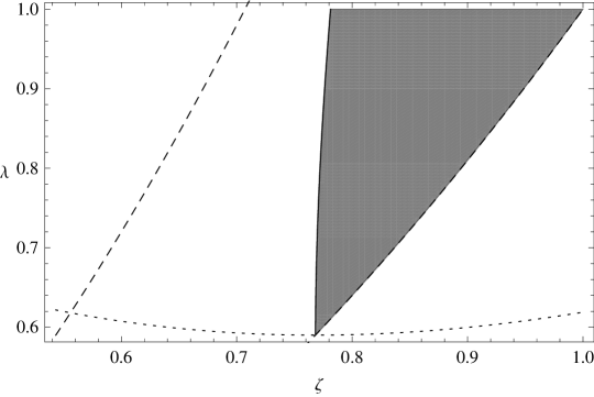
Figure 3.1. Different bounds on $\zeta(\lambda)$. Using Lemma 3.6 we find that $\zeta(\lambda)$ should be between the dashed lines. Numerically, with the help of (3.26) instead of (3.3) we find that $\zeta(\lambda)$ belongs to the shaded area. The dotted line is the graph of $\mu_{1}(\zeta)$.

4. The analysis of ${\mathfrak{k}}_{\lambda}(\nu)$

4.1. Starting point

Recall the operator ${\mathfrak{k}}_{\lambda}(\nu)$ with associated eigenvalues $\{\lambda_{j}(\nu)\}$ defined in (1.8). We will for shortness write $f$ instead of $f_{\zeta(\lambda),\lambda}$ and $\zeta$ instead of $\zeta(\lambda)$ in this section. From the sign of the perturbation and Proposition 3.4 we get:

Proposition 4.1.

Let $\Theta_{0}\leq\lambda\leq 1$. We have the following estimates on the eigenvalues of ${\mathfrak{k}}_{\lambda}(\nu)$:

$$\mu_{j}(\nu)\leq\lambda_{j}(\nu)\leq\mu_{j}(\nu)+\frac{9}{2^{4/3}}\zeta^{2/3}\lambda^{1/3}\biggl{(}\frac{1}{2}-\frac{5(\lambda-\Theta_{0})}{12\zeta^{1/2}\lambda\|u_{1}(\,\cdot\,;\xi_{0})\|_{4}^{2}}\biggr{)}^{1/3}(\lambda-\mu_{1}(\zeta)),$$ (4.1)

and

$$\mu_{1}(\nu)\leq\lambda_{1}(\nu)\leq\mu_{1}(\nu)+\frac{3^{3/4}}{2^{1/2}}\zeta^{1/2}(\lambda-\mu_{1}(\zeta))\bigl{(}\mu_{1}(\nu)/2-\nu\mu_{1}^{\prime}(\nu)/4\bigr{)}^{1/4}.$$ (4.2)

Proof.

The estimate (4.1) is an immediate consequence of (3.26). To show the second estimate (4.2), we notice that

$$\lambda_{1}(\nu)\leq\langle u_{1},{\mathfrak{k}}_{\lambda}(\nu)u_{1}\rangle=\mu_{1}(\nu)+\lambda\|fu_{1}\|_{2}^{2},\leq\mu_{1}(\nu)+\lambda\|f\|_{4}^{2}\|u_{1}\|_{4}^{2},$$

and

$$\|u_{1}\|_{4}^{2}\leq\frac{2^{1/2}}{3^{1/4}}\|u_{1}\|_{2}^{3/2}\|u_{1}^{\prime}\|_{2}^{1/2}\leq\frac{2^{1/2}}{3^{1/4}}\bigl{(}\mu_{1}(\nu)/2-\nu\mu_{1}^{\prime}(\nu)/4\bigr{)}^{1/4}.$$ (4.3)

The first inequality in (4.3) is due to Nagy [12], while the second one follows from (2.13). The upper bound in (4.2) now follows from the upper bound in (3.27). ∎

Lemma 4.2.

If $\nu\not\in\mathfrak{I}(\lambda)$ then $\lambda_{1}(\nu)\geq\lambda$.

Proof.

If $\nu\not\in\mathfrak{I}(\lambda)$ then, by (4.1), we get $\lambda_{1}(\nu)\geq\mu_{1}(\nu)\geq\lambda$. ∎

We continue with some identities.

Proposition 4.3.

Suppose that $\nu_{0}$ is a stationary point for $\lambda_{1}$, i.e.

$$\lambda_{1}^{\prime}(\nu_{0})=0\,.$$ (4.4)

Then we have the following identities:

$$\{\lambda_{1}(\nu_{0})-\nu_{0}^{2}-\lambda f^{2}(0)\}v^{2}_{1}(0;\nu_{0})=2\lambda\int_{0}^{+\infty}v^{2}_{1}(t;\nu_{0})f(t)f^{\prime}(t)\,dt\,,$$ (4.5)

$$\int_{0}^{+\infty}(t-\nu_{0})v^{2}_{1}(t;\nu_{0})\,dt=0\,,$$ (4.6)

$$\|(t-\nu_{0})v_{1}(\,\cdot\,;\nu_{0})\|_{2}^{2}+\lambda\int_{0}^{+\infty}tv^{2}_{1}(t;\nu_{0})f(t)f^{\prime}(t)\,dt=\|v_{1}^{\prime}(\,\cdot\,;\nu_{0})\|_{2}^{2}\,,$$ (4.7)

$$\|v_{1}^{\prime}(\,\cdot\,;\nu_{0})\|_{2}^{2}+\|(t-\nu_{0})v_{1}(\,\cdot\,;\nu_{0})\|_{2}^{2}+\lambda\|f\,v_{1}(\,\cdot\,;\nu_{0})\|_{2}^{2}=\lambda_{1}(\nu_{0})\,.$$ (4.8)

Proof.

Equation (4.5) is a Dauge-Helffer type formula, (4.6) is the Feynman-Hellmann formula, (4.7) follows by the virial theorem and (4.8) is just the energy equation. ∎

Corollary 4.4.

If $0<\zeta<\nu_{0}$, $\lambda_{1}^{\prime}(\nu_{0})=0$ and $\int_{0}^{+\infty}v^{2}_{1}(t;\nu_{0})f(t)f^{\prime}(t)\,dt\geq 0$ then $\lambda_{1}(\nu)>\lambda$.

Proof.

From (4.5) and (3.25) we get

$$\lambda_{1}(\nu_{0})\geq\lambda f(0)^{2}+\nu_{0}^{2}=\lambda+(\lambda-\zeta^{2})+(\nu_{0}^{2}-\zeta^{2})>\lambda,$$

since $\lambda\geq\zeta^{2}$ by (3.39) and $\nu_{0}^{2}>\zeta^{2}$ by the assumption. ∎

Remark 4.5.

From Theorem 1.7 we notice that it is enough to consider $\nu_{0}>1.33$ and so the condition on $\nu_{0}$ and $\zeta$ is not restricting since $\zeta<1$.

It is also worth to notice that if $\int_{0}^{+\infty}v^{2}_{1}(t;\nu_{0})f(t)f^{\prime}(t)\,dt<0$ then also

$$\int_{0}^{+\infty}tv^{2}_{1}(t;\nu_{0})f(t)f^{\prime}(t)\,dt<0,$$

since there exists a $t_{0}$ such that $f^{\prime}(t)$ is positive for $t\in\left]0,t_{0}\right[$ and negative for $t\in\left]t_{0},\infty\right[$, see [11].

4.2. Lower bound on $\lambda_{1}(\nu)$

Lemma 4.6.

If $\lambda_{2}(\nu)>\lambda+(\nu-\zeta)^{2}$ then it holds that

$$\lambda_{1}(\nu)\geq\lambda+(\nu-\zeta)^{2}\biggl{[}1-\frac{4\|(t-\zeta)f\|_{2}^{2}}{\bigl{(}\lambda_{2}(\nu)-\lambda-(\nu-\zeta)^{2}\bigr{)}\|f\|_{2}^{2}}\biggr{]}.$$ (4.9)

Proof.

The Temple inequality (see [10]) with $f/\|f\|_{2}$ as trial state, implies that if $\lambda_{2}(\nu)>A$ then

$$\lambda_{1}(\nu)\geq A-\frac{B}{\lambda_{2}(\nu)-A},$$ (4.10)

where

$$A=\frac{\langle f,{\mathfrak{k}}_{\lambda}(\nu)f\rangle}{\|f\|_{2}^{2}}=\lambda+(\nu-\zeta)^{2}$$

and

$$B=\frac{\langle f,({\mathfrak{k}}_{\lambda}(\nu)-A)^{2}f\rangle}{\|f\|_{2}^{2}}=\frac{\langle f,{\mathfrak{k}}_{\lambda}(\nu)^{2}f\rangle}{\|f\|_{2}^{2}}-A^{2}.$$

Using that ${\mathfrak{k}}_{\lambda}(\zeta)f=\lambda f$, we find that

$${\mathfrak{k}}_{\lambda}(\nu)f=\lambda f-2(\nu-\zeta)(t-\zeta)f+(\nu-\zeta)^{2}f,$$

and so

$$\|{\mathfrak{k}}_{\lambda}(\nu)f\|^{2}=\bigl{(}\lambda+(\nu-\zeta)^{2}\bigr{)}^{2}\|f\|_{2}^{2}+4(\nu-\zeta)^{2}\|(t-\zeta)f\|_{2}^{2}.$$

We conclude that

$$B=4(\nu-\zeta)^{2}\frac{\|(t-\zeta)f\|_{2}^{2}}{\|f\|_{2}^{2}}.$$

Inserting these expressions for $A$ and $B$ into (4.10) yields (4.9). ∎

Proof of Theorem 1.5.

We only consider (1), since the second item has already been established. Combining the lower bounds on $\|f\|_{4}$ from (3.32) and (3.27) we first get

$$2\|(t-\zeta)f\|_{2}^{2} =\lambda\|f\|_{2}^{2}-\frac{3\lambda}{4}\|f\|_{4}^{4}$$ (4.11)

$$\leq\lambda\|f\|_{2}^{2}\Bigl{(}1-\frac{1}{2\zeta^{1/2}}\|f\|_{4}^{2}\Bigr{)}$$

$$\leq\lambda\|f\|_{2}^{2}\biggl{(}1-\frac{\lambda-\Theta_{0}}{2\lambda\zeta^{1/2}\|u_{1}(\,\cdot\,;\xi_{0})\|_{4}^{2}}\biggr{)}.$$

We implement this in (4.9) and use the simple inequality $\lambda_{2}(\nu)\geq\mu_{2}(\nu)$,

$$\lambda_{1}(\nu)\geq\lambda+(\nu-\zeta)^{2}\Biggl{[}\frac{\mu_{2}(\nu)-\bigl{(}3\lambda-\frac{\lambda-\Theta_{0}}{\zeta^{1/2}\|u_{1}(\,\cdot\,;\xi_{0})\|_{4}^{2}}\bigr{)}-(\nu-\zeta)^{2}}{\lambda_{2}(\nu)-\lambda-(\nu-\zeta)^{2}}\Biggr{]}.$$ (4.12)

By continuity it suffices to check verify that

$$\mu_{2}(\zeta)-\biggl{(}3\lambda-\frac{\lambda-\Theta_{0}}{\zeta^{1/2}\|u_{1}(\,\cdot\,;\xi_{0})\|_{4}^{2}}\biggr{)}>0,$$ (4.13)

and

$$\lambda_{2}(\zeta)-\lambda>0.$$ (4.14)

This last inequality is trivially satisfied since $\lambda_{2}\geq\mu_{2}$ which satisfies the lower bound (2.19). Thus we only have to consider (4.13). Notice that the parenthesis in (4.13) is strictly less than $3$. Since $\mu_{2}$ is decreasing on $\left[0,1\right]$ and $\mu_{2}(1)=3$ this finishes the proof. ∎

Define the set ${\mathcal{X}}(\lambda)\subset{\mathfrak{I}}(\lambda)$ as the possible values of $\zeta$, i.e.

$${\mathcal{X}}(\lambda):=\{\zeta\in{\mathbb{R}}\,:\,\text{ the function }{\mathbb{R}}\ni z\mapsto{\mathcal{F}}_{z,\lambda}(f_{z,\lambda})\text{ has a minimum at }\zeta\}.$$ (4.15)

By Lemma 3.6 we have ${\mathcal{X}}(\lambda)\subset\bigl{[}\sqrt{\lambda/2},\sqrt{\lambda}\,\bigr{]}$, but from Figure 3.1 it actually follows that

$${\mathcal{X}}(\lambda)\subset\bigl{[}\xi_{0},\sqrt{\lambda}\,\bigr{]}$$ (4.16)

We can summarize the result (4.12) of Temple’s inequality as follows

Proposition 4.7.

Let $\Theta_{0}\leq\lambda\leq 1$. Assume that

$$\mu_{2}(\nu)-\biggl{(}3\lambda-\frac{\lambda-\Theta_{0}}{\zeta^{1/2}\|u_{1}(\,\cdot\,;\xi_{0})\|_{4}^{2}}\biggr{)}-(\nu-\zeta)^{2}\geq 0,$$ (4.17)

and

$$\mu_{2}(\nu)-\lambda-(\nu-\zeta)^{2}>0$$ (4.18)

for all $\zeta\in\mathcal{X}(\lambda)$ and $\nu\in\mathfrak{I}(\lambda)$. Then $\lambda_{1}(\nu)\geq\lambda$ for all $\nu\in{\mathfrak{I}}(\lambda)$.

Proof of Theorem 1.7.

We will use Proposition 4.7. We start by verifying (4.18). To prove (i) we need only to consider $0\leq\nu\leq 1.33$ and to prove (ii) it suffices to consider $0\leq\nu\leq 1.5$ since the right endpoint of the interval $\mathfrak{I}(0.8)$ is less than $1.5$ (solving the equation $\mu_{1}(\nu)=0.8$ gives a numerical value $\nu\approx 1.496$). The inequality (4.18) holds for all $0\leq\nu\leq 1.5$, $\zeta\in\mathcal{X}(\lambda)$ and $\Theta_{0}\leq\lambda\leq 1$. Indeed, $(\nu-\zeta)^{2}<1$ by (4.16) and $\mu_{2}(\nu)\geq 2.18$ by (2.19).

We now consider (4.17). If $0\leq\nu\leq\zeta$, $\xi_{0}\leq\zeta\leq 1$ and $\Theta_{0}\leq\lambda\leq 1$ then

$$\mu_{2}(\nu)-3\lambda-(\nu-\zeta)^{2}\geq\mu_{2}(\nu)-3-(\nu-1)^{2}.$$ (4.19)

From Figure B.2 it is clear that $\mu_{2}^{\prime}(\nu)<2(\nu-1)$ on $0\leq\nu\leq 1$. Hence, the function $\nu\mapsto\mu_{2}(\nu)-3-(\nu-1)^{2}$ is decreasing on this interval. Since $\mu_{2}(1)=3$ we find that the right-hand side of (4.19) is bounded from below by $0$, and it follows that (4.17) holds for $\nu\leq\zeta$.

To complete the proof of (i) it is sufficient to show that the inequality (4.17) holds for $\xi_{0}\leq\zeta\leq\sqrt{\lambda}$, $\zeta<\nu\leq 1.33$ and $\Theta_{0}\leq\lambda\leq 1$. From Figure B.1 we note that $\mu_{2}$ is decreasing for these values of $\nu$, and so since $\nu>\zeta$ it follows that the left-hand side in (4.17) is decreasing as a function of $\nu$. Hence we get a lower bound replacing $\nu$ by the right endpoint $1.33$. Moreover, $1.5\approx 3-1/\bigl{(}\xi_{0}^{1/2}\|u(\,\cdot\,;\xi_{0})\|_{4}^{2}\bigr{)}>0$ so we also get a lower bound if we replace $\lambda$ by $1$, i.e.

$$\mu_{2}(\nu)-\biggl{(}3\lambda-\frac{\lambda-\Theta_{0}}{\zeta^{1/2}\|u_{1}(\,\cdot\,;\xi_{0})\|_{4}^{2}}\biggr{)}-(\nu-\zeta)^{2}\\ \geq\mu_{2}(1.33)-\biggl{(}3-\frac{1-\Theta_{0}}{\zeta^{1/2}\|u_{1}(\,\cdot\,;\xi_{0})\|_{4}^{2}}\biggr{)}-(1.33-\zeta)^{2}.$$ (4.20)

Differentiating the right-hand side of (4.20) with respect to $\zeta$ and estimating on $\xi_{0}\leq\zeta\leq 1$ we find

$$\frac{d}{d\zeta}\biggl{[}\mu_{2}(1.33)-\biggl{(}3-\frac{1-\Theta_{0}}{\zeta^{1/2}\|u_{1}(\,\cdot\,;\xi_{0})\|_{4}^{2}}\biggr{)}-(1.33-\zeta)^{2}\biggr{]}$$

$$\begin{aligned} &=-\frac{1-\Theta_{0}}{2\zeta^{3/2}\|u_{1}(\,\cdot\,;\xi_{0})\|_{4}^{2}}+2(1.33-\zeta)\\ &\geq-\frac{1-\Theta_{0}}{2\xi_{0}^{3/2}\|u_{1}(\,\cdot\,;\xi_{0})\|_{4}^{2}}+2(1.33-1)\\ &\approx 0.26.\end{aligned}$$

Thus, we get a lower bound of the right-hand side of (4.20) by inserting the left endpoint $\zeta=\xi_{0}$. The lower bound is

$$\mu_{2}(1.33)-\biggl{(}3-\frac{1-\Theta_{0}}{\xi_{0}^{1/2}\|u_{1}(\,\cdot\,;\xi_{0})\|_{4}^{2}}\biggr{)}-(1.33-\xi_{0})^{2}\approx 0.01.$$

This finishes the proof of (i).

We continue with (ii). It is sufficient to show that the inequality (4.17) holds for $\xi_{0}\leq\zeta\leq\sqrt{\lambda}$, $\zeta<\nu\leq 1.5$ and $\Theta_{0}\leq\lambda\leq 0.8$, where the endpoint $1.5$ is chosen to be slightly larger than the right endpoint of the interval $\mathfrak{I}(0.8)$.

Again $\mu_{2}$ is decreasing for these values of $\nu$, and so since $\nu>\zeta$ it follows that the left-hand side in (4.17) is decreasing as a function of $\nu$. Hence we get a lower bound replacing $\nu$ by $1.5$. In the same way as for (i) we also get a lower bound if we replace $\lambda$ by the right endpoint $0.8$, i.e.

$$\mu_{2}(\nu)-\biggl{(}3\lambda-\frac{\lambda-\Theta_{0}}{\zeta^{1/2}\|u_{1}(\,\cdot\,;\xi_{0})\|_{4}^{2}}\biggr{)}-(\nu-\zeta)^{2}\\ \geq\mu_{2}(1.5)-\biggl{(}3\times 0.8-\frac{0.8-\Theta_{0}}{\zeta^{1/2}\|u_{1}(\,\cdot\,;\xi_{0})\|_{4}^{2}}\biggr{)}-(1.5-\zeta)^{2}.$$ (4.21)

We differentiate the right-hand side of (4.21), and estimate for $\xi_{0}\leq\zeta\leq\sqrt{0.8}$, to find

$$\frac{d}{d\zeta}\biggl{[}\mu_{2}(1.5)-\biggl{(}3\times 0.8-\frac{0.8-\Theta_{0}}{\zeta^{1/2}\|u_{1}(\,\cdot\,;\xi_{0})\|_{4}^{2}}\biggr{)}-(1.5-\zeta)^{2}\biggr{]}$$ (4.22)

$$\begin{aligned} &=-\frac{0.8-\Theta_{0}}{2\zeta^{3/2}\|u_{1}(\,\cdot\,;\xi_{0})\|_{4}^{2}}+2(1.5-\zeta)\\ &\geq-\frac{0.8-\Theta_{0}}{2\xi_{0}^{3/2}\|u_{1}(\,\cdot\,;\xi_{0})\|_{4}^{2}}+2(1.5-\sqrt{0.8})\\ &\approx 1.0.\end{aligned}$$ (4.23)

Hence, we get a lower bound of the right-hand side of (4.21) by inserting the left endpoint $\zeta=\xi_{0}$. The lower bound we get is

$$\mu_{2}(1.5)-\biggl{(}3\times 0.8-\frac{0.8-\Theta_{0}}{\xi_{0}^{1/2}\|u_{1}(\,\cdot\,;\xi_{0})\|_{4}^{2}}\biggr{)}-(1.5-\xi_{0})^{2}\approx 0.026.$$

This finishes the proof of (ii). ∎

Appendix A Comments on the numerical calculations

We give some details on how the numerical calculations were done. The solutions to the eigenvalue equation $\mathfrak{h}(\xi)u=\mu(\xi)u$, not taking the Neumann boundary condition into account, are given by

$$u(t)=c_{1}e^{-\frac{1}{2}(t-\xi)^{2}}H_{\frac{1}{2}(\mu(\xi)-1)}(t-\xi)+c_{2}e^{\frac{1}{2}(t-\xi)^{2}}H_{-\frac{1}{2}(\mu(\xi)+1)}(i(t-\xi)).$$ (A.1)

Here, $H_{\nu}(t)$ solves the Hermite equation (see Section 10.13 in [4])

$$-y^{\prime\prime}(t)+2ty^{\prime}(t)-2\nu y(t)=0,$$

and is polynomially bounded at infinity. Hence, for the function $u$ in (A.1) to be square integrable, we must set $c_{2}=0$. Using the well-known relations for the derivative of $H_{\nu}$, $\frac{d}{dt}H_{\nu}(t)=2\nu H_{\nu-1}(t)$, we find that the Neumann condition $u^{\prime}(0)=0$ reads

$$(\mu(\xi)-1)H_{\frac{1}{2}(\mu(\xi)-3)}(-\xi)+\xi H_{\frac{1}{2}(\mu(\xi)-1)}(-\xi)=0.$$ (A.2)

Hence, for $\xi\in\mathbb{R}$, the $j$th eigenvalue $\mu_{j}(\xi)$ of the operator $\mathfrak{h}(\xi)$ is given by the $j$th (positive) solution $\mu(\xi)$ of (A.2). To obtain an equation for $\mu_{j}^{\prime}(\xi)$ we differentiate (A.2) implicitly.

We use the software Mathematica from Wolfram Research (who claims that Mathematica is able to calculate these special functions to any given precision) to solve these equations numerically and draw the plots. By inserting (2.5) into (A.2) we are also able to calculate the constant $\Theta_{0}$ to any precision (see also Remark A.6 in [7]).

Appendix B Additional graphs

In this appendix we have collected some additional graphs that have to do with the eigenvalues $\mu_{j}(\xi)$ of $\mathfrak{h}(\xi)$.

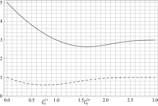
Figure B.1. A plot of $\mu_{1}$ (dashed) and $\mu_{2}$ (solid).

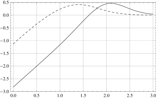
Figure B.2. A plot of $\mu_{1}^{\prime}$ (dashed) and $\mu_{2}^{\prime}$ (solid).

References

- [1] Y. Almog and B. Helffer. The distribution of surface superconductivity along the boundary: on a conjecture of X. B. Pan. SIAM J. Math. Anal., 38(6):1715–1732 (electronic), 2007.
- [2] C. Bolley and B. Helffer. An application of semi-classical analysis to the asymptotic study of the supercooling field of a superconducting material. Ann. Inst. H. Poincaré Phys. Théor., 58(2):189–233, 1993.
- [3] M. Dauge and B. Helffer. Eigenvalues variation. I. Neumann problem for Sturm-Liouville operators. J. Differential Equations, 104(2):243–262, 1993.
- [4] A. Erdélyi, W. Magnus, F. Oberhettinger, and F. G. Tricomi. Higher transcendental functions. Vol. II. Robert E. Krieger Publishing Co. Inc., Melbourne, Fla., 1981. Based on notes left by Harry Bateman, Reprint of the 1953 original.
- [5] S. Fournais and B. Helffer. Spectral Methods in Surface Superconductivity, volume 77 of Progress in Nonlinear Differential Equations and Their Applications. Birkhäuser, to appear in 2010.
- [6] S. Fournais and A. Kachmar. Nucleation of bulk superconductivity close to critical magnetic field. arXiv:0909.5451v1, 2009.
- [7] S. Fournais and M. Persson. Strong diamagnetism for the ball in three dimensions. arXiv:0911.4838v1, 2009.
- [8] B. Helffer. The Montgomery model revisited. Colloquium Mathematicum, volume in honor of A. Hulanicki, 118(2):391–400, 2010.
- [9] B. Helffer and M. Persson. Spectral properties of higher order anharmonic oscillators. Journal of Mathematical Sciences, 165(1), 2010.
- [10] T. Kato. On the upper and lower bounds of eigenvalues. J. Phys. Soc. Japan, 4:334–339, 1949.
- [11] X.-B. Pan. Surface superconductivity in applied magnetic fields above . Comm. Math. Phys., 228(2):327–370, 2002.
- [12] B. Sz.-Nagy. Über Integralgleichungen zwischen einer Funktion und ihrer Ableitungen. Acta Sci. Math. Szeged, 10:64–74, 1941.