The X-ray spectrum of the newly discovered accreting millisecond pulsar IGR J17511–3057

Abstract

We report on a 70ks XMM-Newton ToO observation of the newly discovered accreting millisecond pulsar, IGR J17511–3057. Pulsations at 244.8339512(1) Hz are observed throughout the outburst with an RMS pulsed fraction of 14.4(3)$\%$. Pulsations have been used to derive a precise solution for the P${}_{orb}=12487.51(2)$s binary system. The measured mass function indicates a main sequence companion star with a mass between 0.15 and 0.44 M_⊙.

The XMM-Newton 0.5–11 keV spectrum of IGR J17511–3057 can be modelled by at least three components, which we interpret, from the softest to the hardest, as multicoloured disc emission, thermal emission from the neutron star surface and thermal Comptonization emission. Spectral fit of the XMM-Newton data and of the RXTE data, taken in a simultaneous temporal window, well constrain the Comptonization parameters: the electron temperature, kT_e=51${}^{+6}_{-4}$ keV, is rather high, while the optical depth ($\tau$=1.34${}^{+0.03}_{-0.06}$) is moderate.

The energy dependence of the pulsed fraction supports the interpretation of the cooler thermal component as coming from the accretion disc, and indicates that the Comptonizing plasma surrounds the hot spots on the neutron star surface, which in turn provide the seed photons. Signatures of reflection, such as a broadened iron K$\alpha$ emission line and a Compton hump at $\sim 30$ keV, are also detected. We derive from the smearing of the reflection component an inner disc radius of $\;\buildrel>\over{\sim}\;$ 40 km for a 1.4 M_⊙ neutron star, and an inclination between 38^∘ and 68^∘.

XMM-Newton also observed two type-I X-ray bursts, whose fluence and recurrence time suggest that the bursts are ignited in a nearly pure helium environment. No photospheric radius expansion is observed, thus leading to an upper limit on the distance to the source of 10 kpc. A lower limit of 6.5 kpc can be also set if it is assumed that emission during the decaying part of the burst involves the whole neutron star surface. Pulsations are observed during the burst decay with an amplitude similar to the persistent emission. They are also compatible with being phase locked to pre-burst pulsations, suggesting that the location on the neutron star surface where they are formed does not change much during bursts.

1 Introduction

The discovery of 244.8 Hz pulsations in the X-ray emission of the newly discovered transient source, IGR J17511–3057 (Markwardt et al., 2009), has brought to thirteen the number of Accreting Millisecond Pulsars (hereafter AMSP) discovered so far. Such high spin frequencies are believed to ensue from a long phase ($\lower 2.15277pt\hbox{$\;\buildrel>\over{\sim}\;$}10^{8}$ yr) of accretion of mass and angular momentum onto the neutron star (NS), according to the so-called recycling scenario (Bhattacharya & van den Heuvel, 1991).

In this paper we mainly focus on the spectral properties of this source. The broadband continuum of AMSP has been invariably found to be dominated by a power-law like hard emission with a cut off at an energy between 30 and 60 keV . This emission is interpreted as Comptonization of soft photons in a hot plasma (see Poutanen, 2006, and references therein, for a review of the spectral properties of AMSP). At energies of $\sim$1 keV two soft components are also generally found (Gierliński & Poutanen 2005, GP05 hereinafter, Papitto et al. 2009; Patruno et al. 2009). The cooler one is attributed to the accretion disc emission, while the hotter is interpreted as thermal emission of the hotspots on the NS surface. In this scenario, the hotspot thermal emission constitutes the bulk of soft photons that Compton down-scatter the hot plasma. The X-ray spectrum of IGR J17511–3057 is found consistent with this phenomenological description and the outlined physical interpretation fits well the observed spectral properties.

Figure 1: 2–60 keV light curve of the IGR J17511–3057 outburst as observed by the PCU2 of the PCA aboard RXTE. Circles and crosses refer to observations pointed towards IGR J17511–3057 (Obsid P94041) and XTE J1751–305 (Obsid P94042), respectively. As the two PCA fields of view greatly overlap, the detected pulse frequency is used to discriminate from which source the emission observed by the PCA was actually coming from (see text for details). To which source the emission is attributed is indicated at the top of the figure. The time at which the XMM-Newton observation was performed is also shown.

A couple of AMSP have also showed the typical clues of disc reflection, a Compton hump at $\sim 30$ keV (Gierliński et al., 2002) and a K$\alpha$ emission iron line (Papitto et al., 2009; Cackett et al., 2009; Patruno et al., 2009). In particular the line observed from SAX J1808.4–3658 is compatible with the typically broadened shape caused by the relativistic Keplerian motion of the inner rings of the accretion disc, immersed in the deep gravitational well of the compact object (Fabian et al., 1989). The observation of similar broadened lines from AMSPs has a peculiar importance in the context of NS accretors. It may constrain in fact where the magnetosphere breaks off the accretion disc flow and lifts off matter to the accretion columns.

The spectral and timing capabilities of XMM-Newton already proved fundamental to investigate the X-ray emission and pulse properties of AMSPs especially at low energies, as well as to detect iron emission lines at a high statistics. To these ends, we have obtained a 70ks Target of Opportunity (ToO) observation of IGR J17511–3057, performed roughly one week after the outburst onset. We report on the spin and orbital properties of the source in Sec. 3.1, and on its spectrum in Sec.3.3. We also show how it is possible to take advantage of a simultaneous Rossi X-ray Timing Explorer (RXTE) observation, in order to constrain its high energy emission (Sec. 3.3).

Also two type I X-ray bursts were caught by XMM-Newton, making this observation particularly rich (Sec.4). We observed burst oscillations during the bursts, at the same frequency of the non-burst emission. It is of key importance to observe burst oscillations from sources, the rotational state of which is known at a great accuracy. The comparison with the properties of the non-burst pulsations may in fact assess the physical mechanism that produces oscillations during bursts. These have already been observed to be strongly phase locked to the non-burst oscillations, possibly suggesting that the similarities in their formation are more profound than expected (Watts et al., 2008).

2 Observations and data analysis

The X-ray transient IGR J17511–3057 has been discovered by INTEGRAL on 2009 September 21.140, during its Galactic Bulge monitoring (Baldovin et al., 2009). At that time also the RXTE Proportional Counter Array (PCA) detected a rising X-ray flux activity from the Galactic Bulge. This emission was tentatively attributed to two known nearby transient sources, XTE J1751–305, an AMSP spinning at 435 Hz (Markwardt et al., 2002), and GRS 1747–312. RXTE therefore pointed at the position of XTE J1751–305 to discover that the emission instead originated by a source spinning at $\sim$245 Hz. This made IGR J17511–3057 the twelfth AMSP discovered (Markwardt et al., 2009). A follow up Swift ToO observation constrained the source position at a few arcsec accuracy, obtaining a value $\sim$20 arcmin away from XTE J1751–305, thus confirming the discovery of a new source (Bozzo et al., 2010). A Chandra observation further refined the source position (Nowak et al., 2009), giving the most accurate available estimate as RA=17h 51’ 08.66”, DEC=- 30^∘ 57’  41.0” (1 sigma error of 0.6 arcsec), which is the one we consider in the following.

2.1 XMM-Newton

Figure 2: Pulse phase time delays induced by the orbital motion as a function of the mean orbital longitude. Longitude 0^∘ refers to the passage of the pulsar at the ascending node of the orbit. Residuals with respect to the best fitting orbit model are also over-plotted at a magnified scale (rightmost y-axis). The reduced chi squared of the model is 1.15 over 684 degrees of freedom.

XMM-Newton observed IGR J17511–3057 as a ToO observation for 70ks starting on 2009 September 21.037, $\sim$ 9 days after the source discovery. The XMM-Newton observation is indicated by a horizontal bar in Fig.1, where the RXTE PCA light curve of the outburst is plotted.

The EPIC-pn camera operated in timing mode to allow the temporal resolution (30 $\mu$s) needed to study the millisecond variability of the source, and to avoid spectral deformations due to pile-up. Also EPIC-MOS2 camera observed in timing mode, while EPIC-MOS1 operated in Small Window to provide an image of the source. No evident background due to soft proton flares was recorded during the observation, and the full exposure window is retained for scientific purposes. XMM-Newton detected two type I X-ray bursts during its pointing. When analysing the persistent emission, we discarded 20s prior and 110s after the burst onset. This choice is fairly conservative as the e-folding factor of the burst decay is $\tau\simeq 11$s (see Sec.4).

XMM-Newton data have been extracted and reduced using SAS v.9.0. A concatenated and calibrated event file has been created with the task epproc, specifying the Chandra coordinates of the source. The EPIC-pn spectrum has been extracted from a 13 pixels wide region around the source position (RAWX=36), equivalent to 53.3 arcsec (which should encircle more than 90 per cent of the source counts up to 9 keV) A similar stripe centred on RAWX=10 has been used to estimate the background. The background subtracted 1.4–11 keV persistent count rate recorded by the EPIC-pn is 43.9 c/s on the average. Pile up is therefore not an issue for EPIC-pn data. Spectral channels have been re-binned to have at least three channels per resolution element and 25 counts per channel.

EPIC-MOS1 data have been extracted using the task emproc to provide a 101”$\times$101” image of the source. Using the task edetect_chain, we estimate the source position as RA=17h 51m 08.55s, DEC=-30^∘ 57’ 41.7”, with an uncertainty of 4.3 arcsec. This is consistent with the more accurate Chandra determination. EPIC-MOS 2 data have a significantly lower statistics than that of EPIC-pn and are therefore discarded from the spectral analysis.

Reflection Grating Spectrometers (RGS) operated in standard spectroscopy mode and data have been reduced using the task rgsproc. We consider only first order spectra, re-binned in order to have at least 25 counts per channel. The average persistent count rate is 0.4 and 0.5 c/s for RGS1 and RGS2, respectively.

All spectral fits were performed using XSPEC v.12.5.1

2.2 RXTE

Similarly to the other AMSPs, only one third of the X-ray flux of IGR J17511–3057 is emitted in the energy range covered by XMM-Newton. In order to better constrain the broadband X-ray emission, we take advantage of two RXTE observations performed simultaneously to the XMM-Newton pointing, and amounting to an exposure of 8.8ks (Obs. 94041-01-02-08 and Obs. 94041-01-02-18).

RXTE observations have also been used to extract a light curve of the whole outburst. Starting on 2009 September 13.849, RXTE observed IGR J17511–3057 for $\sim$ 24.5 d, achieving a total exposure of 611 ks ($\simeq$30% of the whole outburst; ObsId P94041). The 2–60 keV light curve extracted from the PCU2 of the PCA (Bradt et al., 1993; Jahoda et al., 2006) data is plotted in Fig.1. Background has been subtracted using the faint model (pca_bkgd_cmfaintl7_eMv20051128.mdl), regardless during the outburst the source crosses the threshold of 40 c/s/PCU above which a bright model should be used. Such a choice was made to avoid the unphysical flux discontinuity that would take place when switching from one model to the other. In Fig.1, filled circles represent observations pointed to the IGR J17511–3057 position (ObsId P94041), while crosses refer to pointings in the direction of the nearby source, XTE J1751–305 (ObsId P94042). These two sources are 19.67 arcmin away, and there is an overlap of nearly 80% between the respective PCA pointings (the FWHM of the PCA collimator is $\sim$ 1^∘). RXTE observations are subject to the contribution of both sources, no matter which the instrument is actually pointed to. The detected spin frequency is therefore used to discriminate which source emits the observed flux. As during the first observation reported in Fig.1 the 245 Hz periodicity is detected, it can be attributed to IGR J17511–3057 even if the instrument was pointing towards XTE J1751–305. The overlap between RXTE observations of these two sources becomes even more evident when looking at the late part of the outburst. Around 2009 Oct 8 (Day 26 according to the scale used in Fig.1, where time is reported in days since 2009 Sep 12.0), the X-ray flux shows an increase of more than 70% with respect to the previous emission. Most importantly, 435 Hz pulsations are detected, clearly indicating a renewed activity from XTE J1751–305, as it has also been confirmed by a narrow pointed Swift XRT observation (Markwardt et al., 2009). Observations performed between 2009 Oct 8 and Oct 10 can be therefore safely attributed to a dim outburst of XTE J1751–305, similar to those already displayed in 2005 March (Grebenev et al., 2005) and 2007 April (Falanga et al., 2007).

The fact that IGR J17511–3057 is in the Galactic Bulge not only forces to deal with a crowded field, but also with the Galactic Ridge emission. It is in fact easy to see from Fig.1 that the PCU2 count-rate stays at a level of $\sim$ 6.5 c/s even after the XTE J1751–305 activity episode is over. Emission at the same flux level was observed also at the end of the 2002 outburst of XTE J1751–305 (GP05) and owes to the Galactic ridge. This emission introduces an additional background to all the PCA observations. This is clearly indicated by the prominent 6.6 keV iron line that appears in PCA spectra when this additional background is not accounted for (Markwardt et al., 2009). As we show in Sec.3.3, to subtract this background is of key importance to ensure agreement between the EPIC-pn and RXTE-PCA spectral data. To estimate a reliable spectrum of this additional background we therefore summed up all RXTE data from 2009 Oct 11.400 to 22.745 (for an exposure of 87.8 ks). In the following we refer to this additional background as the Galactic ridge emission.

In order to extract a PCA spectrum, we have considered only data taken by the PCU2, that is the only always switched on during the RXTE observations overlapping with the XMM-Newton pointing. Data processing has also been restricted to its top xenon layer, as it is the less affected by the instrumental background. Only photons in the 3–50 keV band have been retained as this band is best calibrated. Data taken by the High Energy X-ray Timing Experiment (HEXTE, Rothschild et al., 1998) in the 35–200 keV band has been extracted considering the cluster B, which was the only one to perform rocking to estimate the background, at the time the observation took place.

Table 1: Best fitting orbital and spin parameters of IGR J17511–3057 as observed by XMM-Newton. Errors in parentheses are evaluated at 1$\sigma$ confidence level, while upper limits are given at a 3$\sigma$ level.

a $\sin{i}$/c (lt-s)	0.275196(4)
Porb (s)	12487.51(2)
T∗ (MJD)	55094.9695351(7)
e	$<8\times 10^{-5}$
f(M1,M2,i) (M⊙)	$1.07086(5)\times 10^{-3}$
$\nu$ (Hz)	244.8339512(1)
$\dot{\nu}$ (Hz/s)	$<3\times 10^{-11}$

3 The ”persistent” emission

3.1 The pulse profile

In this paper the pulsations shown by IGR J17511–3057 are analysed using only the XMM-Newton data. A temporal analysis based on RXTE data is instead included in a companion paper (Riggio et al., 2010, submitted). In order to perform a timing analysis we retain all the 0.3–12 keV energy interval covered by the EPIC-pn, and report the photons arrival time to the Solar System barycentre using the SAS task barycen, considering the Chandra position given by Nowak et al. (2009). The 244.8 Hz periodicity is clearly detected throughout the XMM-Newton observation. To estimate the spin and orbital parameters we focus on the persistent emission. We first fold 100 s long intervals around the best estimate of the spin frequency given by Riggio et al. (2009). The pulse profiles thus obtained are modelled with a sum of harmonic functions:

$$F(\phi)=A_{0}\left\{1+\sum_{k}A_{k}cos[k(\phi-\phi_{k})]\right\}$$ (1)

where $A_{0}$ is the average countrate, $\phi=2\pi\nu(t-T_{0})$ is the rotational phase, and $A_{k}$ and $\phi_{k}$ are the fractional amplitude and phase of the k-th harmonic, respectively. Two harmonics are enough to model pulse profiles obtained over 100s intervals. The relevant orbital parameters (the semi-major axis of the NS orbit, $x=a\sin{i}/c$, the orbital period, $P_{orb}$, the epoch of passage at the ascending node of the orbit, $T^{*}$, and the eccentricity $e$) are estimated fitting the time delays affecting the first harmonic phases with respect to a constant frequency model (see Eq.(3) of Papitto et al. 2007, and references therein). The observed time delays, together with the residuals with respect to the best fitting model, are plotted in Fig.2, while the orbital parameters we obtain are listed in Table 1. They are perfectly compatible with those estimated by Riggio et al. (2010, submitted) considering the RXTE coverage of the outburst, even if the uncertainties that affect them are naturally larger because of the shorter exposure they are calculated over.

Figure 3: Pulse profile obtained by folding the 0.3–12keV EPIC-pn time series in 64 bins around the best spin frequency estimate, $\nu=244.8339512$, after having corrected data for the orbital motion. The solid line is the best fitting five harmonics function described in text. The first (dashed line), second (dotted line) and third (dash-dotted) harmonic are also over-plotted. An offset equal to the average count rate have been added to the harmonics count-rate for graphical purposes. Two cycles are shown for clarity.

After the photon arrival times have been corrected for the orbital motion of the pulsar, we folded data in 16 phase bins over longer time intervals (1000s), and derived more stringent measures of the phases and of their temporal evolution. The statistical errors on the phases obtained fitting the profiles so obtained are summed in quadrature with the uncertainty introduced by the errors affecting the orbital parameters (see Eq.(4) in Papitto et al. 2007). As there are no significant differences between the estimates we obtain with the two harmonic components, we present here only the results based on the fundamental one. The phase evolution can be successfully modelled by a constant frequency ($\chi^{2}_{red}=1.02$ for 68 d.o.f.), whose estimate is given in Table 1. The quoted error is evaluated considering also the uncertainty introduced by the positional error-box (see Burderi et al. 2007). The introduction of a quadratic term, possibly reflecting a spin evolution of the source, is not significant, and it is possible to derive a 3$\sigma$ upper limit on the spin frequency derivative of $1\times 10^{-11}$ Hz/s.

Figure 4: Variation with energy of the fractional amplitude of the first (top), second (middle) and third (bottom) harmonic.

Folding over the entire observation length the 0.3–12 keV EPIC-pn time series we obtain the average pulse profile plotted in Fig.3. Five harmonics are needed to successfully fit (i.e. $\chi^{2}/$dof=53.1/54) the pulse profile using Eq.(1), while AMSPs pulse profiles are generally fitted by just two components. Such a complexity is unveiled probably thanks to the high statistics and low background granted by the EPIC-pn, and, most importantly, to the larger pulse fraction IGR J17511–3057 shows with respect to the other objects of this class. Accounting for the average background count-rate (2.225(6) in the 0.3–12 keV band), the fractional amplitudes of these harmonic components are in fact, $20.21(8)\%$, $2.66(8)\%$, $0.98(8)\%$, $0.39(8)\%$ and $0.33(8)\%$, respectively, where the errors in parentheses are quoted at 1$\sigma$ confidence level. The total RMS pulsed fraction can be estimated as $(\sum_{k}A_{k}^{2}/2)^{1/2}=14.4(3)\%$ RMS.

The pulse of IGR J17511–3057 also shows strong spectral variability. The amplitude of the first harmonic increases with energy until it reaches an approximately constant value of $\sim 0.22$ at $\sim 3keV$. The second and third harmonic are instead more regular (see Fig. 4). We show in Sec.5.3 how the decrease of the pulsed fraction can be understood in terms of the shape of the various components used to model the X-ray spectrum. Phase lags are also observed (see Fig.5). In particular the phase of the fundamental shows an excursion of $\sim 230\mu s$ (0.06 in phase units) between 1 and 10 keV, with the pulses at low energy lagging those at higher energies. Lags are also shown by the second harmonic, even if their significance is lowered by the larger error bars affecting these estimates, with respect to those calculated on the first harmonic. The behaviour with energy of the second harmonic phases is anyway more regular. While at low energies the second harmonic phase anticipates the first harmonic, at higher energies they become comparable. We thus conclude that the overall pulse shape is energy dependent.

Figure 5: Phases in $\mu s$ of the first (solid line) and second harmonic (dotted line) with respect to energy. An common offset has been set on phases so that the phase of the fundamental between 1 and 2 keV is equal to 0.

Table 2: Fitting parameters of the 0.5-11.0 keV combined RGS + EPIC–pn spectrum of IGR J17511–3057. Models are defined as follows: Model A, phabs$\times$edge(diskbb+bbodyrad+nthcomp) with kT${}_{soft}=$kT_BB; Model B, phabs$\times$edge(diskbb+bbodyrad+nthcomp) with kT${}_{soft}\neq$kT_BB; Model C, same as model Model B with the addition of a diskline to model the K$\alpha$ iron emission feature. The disc outer radius is fixed to $1\times 10^{5}$ R_g. All these models are evaluated for an electron temperature of the Comptonized component fixed to 100 keV. Errors on each parameter are quoted at the 90% confidence level, as for all the spectral parameters in the rest of the paper.

Model	A	B	C
nH ($10^{22}$ cm-2)	$1.10^{+0.07}_{-0.04}$	$0.98\pm 0.04$	$0.96^{+0.01}_{-0.02}$
$\tau$ O VIII	$0.22\pm 0.08$	$0.21\pm 0.07$	$0.20\pm 0.07$
kTin (keV)	$0.21^{+0.02}_{-0.01}$	$0.33^{+0.04}_{-0.02}$	$0.34^{+0.04}_{-0.03}$
R${}_{in}(\cos{i})^{1/2}$ ($d_{8}$ km)	$63^{+28}_{-19}$	$20^{+5}_{-4}$	$17^{+4}_{-5}$
kTBB (keV)	$0.39^{+0.02}_{-0.03}$	$0.62^{+0.03}_{-0.02}$	$0.63^{+0.02}_{-0.03}$
RBB ($d_{8}$ km)	$7\pm 1$	$7.1^{+0.5}_{-0.6}$	$6.7^{+0.3}_{-0.4}$
$\Gamma$	$1.710\pm 0.008$	$2.4\pm 0.2$	$2.1^{+0.2}_{-0.1}$
kTsoft (keV)	=kTBB	$1.5\pm 0.01$	$1.36^{+0.05}_{-0.17}$
EFe (keV)	—	—	$6.72^{+0.24}_{-0.09}$
$\beta$	—	—	$-4.1^{+0.8}_{-2.9}$
Rin ($GM/c^{2}$)	—	—	$37^{+31}_{-9}$
i $(^{\circ})$	—	—	$>37$
EW (eV)	—	—	$43.9\pm 0.06$
$\chi^{2}_{red}$	$2008.1/1598$	$1775.8/1597$	$1740.7/1592$

3.2 The XMM-Newton spectrum

We first analyse the XMM-Newton spectrum, considering data taken by the two RGS (0.5–2.0 keV) and by the EPIC-pn (1.4–11.0 keV). EPIC-pn data below 1.4 keV are discarded as they show a clear soft excess with respect to RGS data, regardless of the model used to fit the spectrum. Such an excess was already noticed by, e.g., Boirin et al. (2005); Iaria et al. (2009); D’Aì et al. (2009); Papitto et al. (2009); D’Aì et al. (2010), analysing observations performed by the EPIC-pn in timing mode. The absence of such a feature in RGS data indicates how it is probably of calibration origin, hence the choice to retain only data taken by the EPIC-on in the 1.4–11.0 keV energy interval, for the purposes of a spectral analysis. The relative normalisation of the RGS1 and RGS2 with respect to the EPIC-pn camera are left free. We find RGS1/PN=$1.02(1)$ and RGS2/PN=$0.98(1)$, regardless of the particular spectral model considered. The numbers quoted in parentheses are the errors at 90% confidence level, level at which the uncertainty on any spectral parameter is quoted in this paper.

The 0.5–11 keV spectrum of IGR J17511–3057 is energetically dominated by a power law, which is easy to interpret as the realization of a broader Comptonized emission on a limited bandwidth. The first Comptonization model we consider is nthcomp (Zdziarski et al., 1996; Życki et al., 1999). It describes a thermal Comptonization spectrum in terms of the temperature of the input soft photons (kT_soft), the temperature of the hot comptonizing electrons (kT_e) and by an asymptotic power law index ($\Gamma$) related to kT_e and to the medium optical depth $\tau$ through the relation:

$$\Gamma=\left[\frac{9}{4}+\frac{1}{\left(\frac{kT_{e}}{m_{e}c^{2}}\right)\tau\left(1+\frac{\tau}{3}\right)}\right]^{1/2}-\frac{1}{2}$$ (2)

(see e.g. Lightman & Zdziarski 1987). As no high energy cut-off appears in the XMM-Newton spectrum, we fix kT_e to an arbitrary value of 100 keV. Such a choice does not affect significantly the results obtained on the XMM-Newton dataset alone. Interstellar absorption is treated with the phabs model, the abundances are fixed at the values of Anders & Grevesse (1989), and cross sections are taken from Balucinska-Church & McCammon (1992), and modifications after Yan et al. (1998). Data show no significant deviation from solar abundances. The nthcomp component alone, poorly reproduces the observed spectrum ($\chi^{2}_{red}=1.68$ for 1604 d.o.f.). Residuals around 1.8 and 2.2 keV are evident. As there is no sign of similar features in the RGS spectra, we interpret them in terms of an incorrect calibration of the instrumental Si and Au edges that frequently affect EPIC-pn spectra. An improvement of $\Delta\chi^{2}=151$ is obtained modelling these residuals with narrow Gaussian absorption features.

As a soft excess is present, we add two thermal components to the model, accordingly to the results previously obtained modelling XMM-Newton spectra of AMSP (GP05, Papitto et al. 2009). We model the softer component as disc emission (diskbb), and the hotter as a single temperature blackbody (bbodyrad). As the normalisation of the latter component is smaller than $\approx$ 10 km, we interpret it as thermal emission arising from the neutron star surface. Assuming that it is this component that provides the seed photons for Comptonization, we tie kT_soft to the temperature of the blackbody. The addition of these two thermal components definitely improves the fit, as the $\chi^{2}$ decreases of 39 and 486, for the addition of two and one degree of freedom, respectively. An absorption edge at $0.88\pm 0.01$ keV is also clearly detected in the RGS data, with an absorption depth of $0.22\pm 0.06$. We identify it as an absorption edge of O VIII (E${}_{\>OVIII}=0.871$ keV). The edge is quite sharp, as an upper limit of $34$ eV is found on its width, if a smeared edge (smedge) is used to model it. The best fitting parameters of this model (named as model A) are listed in the left column of Table 2.

The final reduced chi squared is anyway still large, $\chi^{2}_{red}$=1.26(1598 d.o.f.). Disentangling the temperature of the seed photons of the Comptonized component from the observed blackbody (model B, see Table 2), significantly improves the fit ($\Delta\chi^{2}=232$ for the addition of just one d.o.f.). Data thus favour a hotter and smaller region to produce the seed photons of the Comptonized component, than that of the observed blackbody.

The presence of residuals around 6.6 keV (see Fig.6 where EPIC-pn residuals with respect to a simple power law are plotted in the bottom panel) suggests the presence of an iron K$\alpha$ emission line. Adding a Gaussian centred at $E_{Fe}=6.65\pm 0.25$ keV improves the $\chi^{2}$ by 23 (for three additional d.o.f.). The width of the feature ($\sigma>0.56$ keV) indicates it could be produced from reflection of the NS hard emission on the geometrically thin, optically thick, accretion disc. In this context, the feature is broadened by the relativistic motion of the reflecting plasma in the inner parts of the accretion disc, where the space-time is bent by the gravitational influence of the compact object. We use a diskline model to account for relativistic effects (Fabian et al., 1989), obtaining an improvement of $\Delta\chi^{2}=13$ for 3 d.o.f. added. The diskline model describes the line shape in terms of the size of the illuminated disc (that is, of its inner radius, $R_{in}$, and of its outer radius, $R_{out}$), of the index of the radial dependence of the line emissivity, $\beta$, and of the inclination of the system, $i$. As $R_{out}$ is poorly constrained by the available statistics, we fix it to an arbitrary value of $10^{5}$ R_g (where $R_{g}=GM_{1}/c^{2}$ is the NS gravitational radius, and $M_{1}$ the mass of the compact object), of the order of the circularization radius for a system like IGR J17511–3057 (see e.g. Frank et al., 2002). The parameters we obtain are listed in the rightmost column of Table 2 (model C), and are compatible with the assumption that the line is emitted by plasma illuminated by the NS emission, and rotating in the accretion disc. The energy of the transition indicates mildly to highly ionised iron. As we show in the next section, these indications are supported also by the modelling of disc reflection on a broader energy range. The feature stands at 3.5$\sigma$ above the continuum, and the F probability that the $\chi^{2}$ improvement when switching from model B to model C is due to chance is $<10^{-5}$. However, the use of an F-Test to test the presence of additional components has been strongly discouraged by Protassov et al. (2002, but see also ). We have then simulated 100 spectra starting from the best fit parameters of model B, and fitted them using both model B and C. In none of the cases we have noticed a $\chi^{2}$ improvement, or an F statistics value, larger than the one we obtain from modelling real data. We therefore exclude at more than 99 per cent confidence level that the $\chi^{2}$ improvement obtained with model C with respect to model B is due to chance.

Model C is the best model we have found to fit the XMM-Newton dataset. However the $\chi^{2}$ corresponding to this model is relatively large and the probability that we observe by chance a $\chi^{2}$ equal or larger than the value we obtain, if the model is correct, is 0.5 per cent. This makes the model only barely acceptable. The average scatter of data points with respect to this model is anyway compatible with the accuracy of the effective area calibration of the EPIC-pn, while operated in fast modes (quoted to be better than 5% from an analysis of the 1.5–3 keV band, see http://xmm2.esac.esa.int/docs/documents/CAL-TN-0083.pdf). Since the distribution of residuals does not show any systematic trend, but are instead randomly distributed around what is predicted by our best fit model, we conclude that the $\chi^{2}$ we obtain is affected by uncertainties in the instrument calibration, and/or by the possible presence of unresolved and unfitted features. We therefore retain model C as a reliable description of IGR J17511-3057 spectrum in the considered bandwidth.

3.3 A simultaneous RXTE–XMM-Newton spectrum

The spectrum of IGR J17511–3057 is dominated by a power-law like component which we have interpreted in terms of Comptonization, with a cut-off temperature beyond the energy band covered by the EPIC-pn. Moreover, the detection of a broadened K$\alpha$ iron emission feature indicates how disc reflection may be important. To better assess these issues, we take advantage of the observations performed by RXTE (3–200 keV) overlapping with the XMM-Newton pointing. We thus added to the XMM-Newton data presented in the previous section, the PCA (3–50 keV) and the HEXTE (35–200 keV) spectra. A systematic error of 0.5% has been added to the PCA points according to the guidelines stated in the description of the latest PCA response matrix generator .

In order to check the inter calibration between the EPIC-pn and RXTE-PCA spectra, we simultaneously fit these two spectra with an absorbed power law. The RXTE-PCA spectrum shows large swings up to $\sim$ 10$\sigma$ with respect to EPIC-pn points, with a clear soft excess below 5 keV and a much more prominent emission feature at $\sim$ 6.6 keV. In order to investigate if such a discrepancy could be due to the contamination of the Galactic ridge emission, we subtracted from PCA data the Galactic ridge spectrum (see Sec.2.2). A great improvement ($\Delta\chi^{2}=376.33$ for 710 d.o.f.) is achieved with respect to the unsubtracted data. Most importantly, the residuals of the EPIC-pn and the PCA points are distributed in the same way after the subtraction of the Galactic ridge contribution to the PCA spectrum (see Fig. 6). Such a result gives us confidence about the reliability of the combined XMM-Newton–RXTE spectral modelling we describe in the following. The relative normalisations between the various instruments and the EPIC-pn are left free. The same normalisations quoted in the previous section have been found for the RGS, while PCA/PN and HEXTE/PN vary in the ranges $1.24$–$1.25$ and $0.6$–$0.8$, respectively, depending on the particular model used. We note that the values taken by the normalisation factors for different spectral models are all compatible with each other within the respective errors (that are typically $0.006$ and $0.1$ for PCA/PN and HEXTE/PN, respectively).

Figure 6: Residuals of the RXTE-PCA (top panel) and of the EPIC-pn (bottom panel ) with respect to an absorbed power law model. The RXTE-PCA points are subtracted from an additional background representing the emission of the Galactic ridge.

Table 3: Best-fitting parameters of the 0.5–200 keV spectrum composed of the RGS (0.5–2.0 keV), EPIC-pn (1.4–11 keV), PCA (3.0–50.0 keV) and HEXTE (35–200 keV) spectra. The continuum models are defined as follows: (i) Model B, phabs$\times$edge(diskbb+bbodyrad +nthcomp); (ii) Model B-Refl, phabs$\times$edge(diskbb+bbodyrad+nthcomp+diskline+rdblur$\times$pexriv); (iii) Model PS, phabs$\times$edge(diskbb+bbodyrad+compps); (iv) Model PS-Refl, phabs$\times$edge(diskbb+bbodyrad+compps+diskline+rdblur$\times$pexriv). All the fluxes calculated are unabsorbed.

Model	B	B-Refl	PS	PS-Refl
nH ($10^{22}$ cm-2)	$1.04^{+0.04}_{-0.05}$	$0.98_{-0.05}^{+0.04}$	$1.00^{+0.03}_{-0.04}$	$0.95^{+0.02}_{-0.03}$
$\tau$ O VIII	$0.22^{+0.07}_{-0.08}$	$0.14\pm 0.08$	$0.22\pm 0.07$	$0.19\pm 0.07$
kTin (keV)	$0.27^{+0.03}_{-0.02}$	$0.32^{+0.05}_{-0.02}$	$0.31^{+0.03}_{-0.02}$	$0.36\pm 0.02$
R${}_{in}\sqrt{\cos{i}}$ ($d_{8}$ km)	$33\pm 9$	$19\pm 8$	$24^{+7}_{-4}$	$15^{+1}_{-2}$
F${}_{Disc}^{bol}$($\times 10^{-9}$erg/cm2/s)	$0.20$	$0.13$	$0.17$	$0.14$
kTBB (keV)	$0.53^{+0.02}_{-0.01}$	$0.60\pm 0.04$	$0.60\pm 0.02$	$0.64^{+0.01}_{-0.02}$
RBB ($d_{8}$ km)	$8.7^{+0.6}_{-0.7}$	$6.8\pm 0.6$	$7.6\pm 0.5$	$6.3^{+0.3}_{-0.1}$
F${}_{BB}^{0.5-150}$($\times 10^{-9}$erg/cm2/s)	$0.10\pm 0.02$	$0.10\pm 0.02$	$0.10\pm 0.01$	$0.11\pm 0.01$
$\Gamma$	$1.86^{+0.03}_{-0.02}$	$1.78\pm 0.02$	—	—-
kTel(keV)	$100$(fixed)	$100$(fixed)	$75^{+11}_{-10}$	$51^{+6}_{-4}$
$\tau$	$0.6$–$1.9$	$1.1$–$2.0$	$1.18^{+0.08}_{-0.07}$	$1.34^{+0.03}_{-0.06}$
i${}_{SLAB}(^{\circ})$	—	—	$65.0(fixed)$	$57.0^{+11}_{-7}$
kTsoft	$1.01^{+0.04}_{-0.05}$	$1.1\pm 0.1$	$1.47\pm 0.06$	$1.37^{+0.01}_{0.02}$
Rsoft($d_{8}$ km)	$4.2$–$5.3$	$3.2$–$4.7$	$3.3^{+0.3}_{-0.2}$	$3.4^{+0.1}_{-0.4}$
F${}_{C}^{(0.5-150)}$($\times 10^{-9}$erg/cm2/s)	$1.00\pm 0.04$	$1.04\pm 0.07$	$1.30\pm 0.08$	$1.00\pm 0.05$
$\log\xi$	—	$3.4\pm 0.5$	—	$3.0^{+0.4}_{-0.2}$
$\Omega/2\pi$	—	$0.18\pm 0.05$	—	$0.14^{+0.10}_{-0.01}$
F${}_{Refl}^{(0.5-150)}$($\times 10^{-9}$erg/cm2/s)	—	$0.07\pm 0.02$	—	$0.07\pm 0.03$
EFe (keV)	—	$6.8^{+0.2}_{-0.1}$	—	$6.82^{+0.09}_{-0.11}$
$\beta$	—	$-6_{-6}^{+3}$	—	$-5.5^{+0.8}_{-4.9}$
Rin ($GM/c^{2}$)	—	$22^{+9}_{-5}$	—	$27^{+6}_{-9}$
i $(^{\circ})$	—	$41_{-5}^{+8}$	—	$48^{+6}_{-10}$
EW (eV)	—	$35\pm 1$	—	$40.9\pm 0.7$
F${}_{unabs}^{0.5-150}$($\times 10^{-9}$erg/cm2/s)	$1.19\pm 0.04$	$1.28\pm 0.08$	$1.52\pm 0.08$	$1.28\pm 0.06$
$\chi^{2}_{red}$	$1993.1/1721$	$1838.1/1713$	$1912.7/1720$	$1847.7/1712$

Figure 7: Unfolded 0.5–200 keV spectrum of IGR J17511–3057 convolved with the model B+refl (left) and PS+Refl (right; see caption of Table 3 for a description), together with residuals in units of sigmas in the respective bottom panels. The overall model (thick solid line), the diskbb (dashed line), the blackbody (solid thin line), the Comptonized spectrum (dotted line), and the reflected spectrum (continuum and diskline, dash-dotted line) are also overplotted. Data have been re-binned for graphical purposes.

As expected, the analysis of the combined datasets gives similar results than those presented in the previous section for what concerns the low energy part of the spectrum. Two soft components are requested to model the observed data, in addition to an $\alpha=1.56\pm 0.04$ power law, cut off at an energy $E=51^{+16}_{-9}$ keV. Using nthcomp to model the hard emission we find that, if the observed blackbody provides the seed photons upscattered in the Comptonizing medium ($kT_{BB}=kT_{soft}=0.34^{+0.03}_{-0.04}$ keV), chi squared is large ($\chi^{2}_{red}=1.26$ for 1722 d.o.f.). Moreover, a region of size larger than the one measured ($R_{BB}=8.6\pm 2.7$ d₈ km, where d₈ is the distance to the source in units of 8 kpc) is needed to provide enough photons for the observed hard component. Such a radius is evaluated considering that the flux escaping the Comptonizing medium is $F^{\prime}=A\times F_{soft}$, where $F_{soft}$ is the seed flux, and the Compton amplification factor is $A=e^{y}$, with $y=(4kT_{e}/m_{e}c^{2})\times\max{(\tau,\tau^{2})}$, the Compton parameter. As the nthcomp model only evaluates the flux added by the Compton process, $F_{C}$, the energy conservation between the two phases can be rephrased as $F_{C}/F_{soft}\simeq e^{y}-1$. Expressing the seed flux as $F_{soft}=\sigma T_{soft}^{4}(R_{soft}/d)^{2}$, the radius of the area providing the seed photons has to be:

$$R_{soft}=2.4\times 10^{5}d_{8}\frac{\sqrt{F_{C}/(e^{y}-1)}}{(kT_{soft})^{2}}km,$$ (3)

where $kT_{soft}$ is expressed in keV. As using nthcomp no significant cut-off is found, we are forced to measure the best-fitting values of $\Gamma$ fixing the electron temperature at values in the range 50–200 keV, and then evaluate $\tau$ and $y$ using Eq.(2). Estimating the flux in the nthcomp component in the 0.5–150 keV energy range, the radius we obtain from Eq.(3) is $R_{soft}\lower 2.15277pt\hbox{$\;\buildrel>\over{\sim}\;$}30$ d₈ km, which is at least a factor $\sim 3$ larger than the normalisation of the observed blackbody component. We thus conclude that the observed blackbody is too cold to be the source of the seed photons.

Letting kT${}_{soft}\neq$ kT_BB improves the modelling by $\Delta\chi^{2}=186$ for the addition of one d.o.f. (see the leftmost column of Table 3 for the best fitting parameters of this model, named as B). As the electron temperature is not constrained by the model, we present the best fitting parameters for kT_el= 100 keV. Using Eq.(3) to evaluate the radius of the unseen thermal component providing the seed photons up-scattered in the Comptonizing medium, we find $R_{soft}\simeq$4–5 d₈ km. This radius is compatible with the expected size of the hotspots on the NS surface.

The presence of an iron K$\alpha$ emission line in the XMM-Newton spectrum indicates a significant presence of reflection. To model Compton reflection from an ionised disc we use the pexriv model (Magdziarz & Zdziarski, 1995). The shape of the power law that describes the illuminating flux is fixed using the index $\Gamma$ of the nthcomp component. The disc temperature is kept fixed at a value of $1\times 10^{6}$ K, the disc inclination at the value indicated by the iron line modelling, and abundances to solar values. The relativity effects expected for a Keplerian accretion disc rotating around a compact object are taken into account with the smearing kernel rdblur (Fabian et al., 1989). To include also the most important bound-bound transition expected (Fe K$\alpha$) in the EPIC-pn range, we add a diskline with a line energy free to vary in the 6.4–6.97 keV interval. The outer radius of the illuminated disc is fixed at $10^{5}$ R_g, as the fit is rather insensitive for variations of this parameter in a wide range of values. The addition of a reflection component is highly significant, as the $\chi^{2}$ improves by 155 for the addition of 9 parameters (see the model BRefl in Table 3 for the best fitting parameters).

As the Comptonization model nthcomp is not able to constrain the electron temperature, the assumption we have made (kT_el=100 keV) has potentially an impact on the amount of reflection needed to model the spectrum. The value of kT_el also influences the determination of the seed-photon region (see Eq. 3). The results obtained considering both the 0.5–11 keV and the 0.5–200 keV energy bands indicate that the seed photons come from a region which is hotter and smaller than the blackbody, and not directly observed. It is then desirable to include in the model those seed photons that are not scattered in the $\tau\approx 1$ Comptonizing medium, as nthcomp only accounts for up-scattered photons. For all these reason, as well as to check the dependence of the measured parameters on the Comptonization model chosen, we substitute nthcomp with compps (Poutanen & Svensson, 1996). This model has in fact a number of advantages with respect to the nthcomp model: (i) it enforces the energy balance between the Comptonizing plasma and the region that provides the soft photons; (ii) it evaluates the Comptonized spectrum by solving numerically the radiative transfer equation, for different scattering orders, and for different geometries of the comptonizing medium. It thus includes those seed photons that go through the hot medium unscattered. We consider in the following a slab geometry; (iii) it uses the pexriv kernel to model disc reflection of the hard photons only. The reflected spectrum thus implicitly takes into account the decrease of photons incident on the disc at low ($\lower 2.15277pt\hbox{$\;\buildrel<\over{\sim}\;$}2$ keV) energies, while using the model B-Refl the incident spectrum is approximated as a power law extending to low energies.

When reflection is not included in the model we obtain the results listed in Table 3 (Model PS). The continuum parameters do not vary much when using this Comptonization model. In particular, the size of the region that provides the seed photons confirms the results previously obtained. Using this model, we are also able to constrain the electron temperature of the hot medium, in agreement with the cut off energy found using a simple power law to model the hard emission.

The property (ii) quoted above introduces a dependence of the emergent spectrum on the angle i_slab between the slab normal and the line of sight. Keeping $i_{slab}$ as a free parameter in spectral fitting yields values $\lower 2.15277pt\hbox{$\;\buildrel>\over{\sim}\;$}80^{\circ}$, that would imply the presence of eclipses, which are instead not observed. As we see in the following, smaller values are obtained when reflection is included into the model. To calculate the spectrum presented in Table 3 we thus fix $i_{slab}=65^{\circ}$. The tendency of the compps model to find large values of $i_{slab}$ when reflection is not included, can be tentatively interpreted as an indirect indication of how reflection is significant to model the broad band spectrum. As a matter of fact, without reflection, a larger flux has to be accounted for by the Comptonized component. As GP05 pointed out, at moderate optical depths like the ones we detect in IGR J17511–3057 ($\tau\approx 1$), the Comptonization spectrum depends on $i_{slab}$ mainly in terms of the amount of unscattered photons observed, $\propto exp(-\tau/cos\;{i_{slab}})$. For these optical depths the angular dependence of the scattered photons is indeed rather flat (see the curves relative to angles $\lower 2.15277pt\hbox{$\;\buildrel<\over{\sim}\;$}70^{\circ}$ in Fig. 4 of Sunyaev & Titarchuk 1985). As the spectral shape (hence kT_soft) is well constrained by data at low energies, it seems that compps gives account of the large flux at high energies assuming that we see the slab at very large angles. In this way only a very small fraction of the unscattered photons would be observed and the total amount of seed photons would be as large as requested to ensure energy balance between the hot and the cold phase. Besides the significant improvement of the model when reflection is included (see rightmost column of Table 3, model PS-Refl), the fact that such an overestimate of $i_{slab}$ is not needed when the addition of reflection decreases the flux at high energies owing to Comptonization, definitely supports its presence.

The parameters of the iron line we find with model PS-Refl are all compatible with those found when Comptonization is described by nthcomp. Also the ionisation state and the amplitude of reflection indicated by the reflection model are consistent within the errors. The models B-refl and PS-refl are plotted in Fig.7 together with residuals. The addition of a reflection component and of an iron line to models B and PS gives values of the F-statistics $>7$. In order to test if such an improvement may be due to statistical fluctuations, we have repeated the procedure described in Sec.3.3, simulating 100 fake spectra using the best fit parameters of the models without reflection features. As we have never obtained an F-statistics value similar to that quoted above, when the reflection features are added to the model, we conclude at more than 99% confidence level that the improvement obtained with their addition is not due to counting statistics.

The best fit models presented for the combined RXTE-XMM-Newton dataset are only barely acceptable (null hypothesis probability of 1.8% and 1.2% for the models B-Refl and PS-Refl, respectively). Similarly to what has been noted in the previous section, the absence of systematic trends in the residuals leads us to conclude that the reduced chi squared is increased by uncertainties in the instruments calibration and/or by the possible presence of unresolved and unfitted features. The fact that models obtained from a fit of five different instruments give indeed fairly satisfactory results seems anyway worthwhile to note, and gives confidence about their reliability.

4 The burst emission

Figure 8: Countrate recorded by the EPIC-pn in the 0.3–12 keV interval (a), apparent radius (b) and temperature (c) of the best fitting absorbed blackbody, fractional amplitude (d) and phase of the pulse first harmonic (e), during the first burst observed by the EPIC-pn. Time is given in seconds since the burst onset (MJD 55095.05025). The values taken by the countrate, the radius and the temperature of the blackbody component of model PS-Refl, during the persistent emission are also over-plotted as dashed lines for comparison.

IGR J17511–3057 exhibited two type I X-ray bursts during the XMM-Newton pointing, sharing similar observational properties (see Table 4). While the rise lasts for $\sim 2$ s, the decay follows an exponential decay ($\chi^{2}_{red}=$0.96 and 1.20, respectively, over 216 d.o.f.; see the top panel of Fig.8 for the light curve of the first burst). In order to study their temporal evolution, we extracted spectra over time intervals or variable length (from 1s at the beginning to 8s at the end), subtracting as a background the persistent spectrum analysed in the previous section. Pile-up is not of concern, as it affects energies $\lower 2.15277pt\hbox{$\;\buildrel>\over{\sim}\;$}8$ keV for at most few per cent. We have anyway checked that the spectrum extracted without the brightest CCD column gives spectral model parameters compatible with those quoted hereafter. We successfully model the burst emission with an absorbed black body. The absorption column has been varied in the range indicated by the various models we have used to model the persistent spectrum. The evolution of the temperature and of the emission radius of the first burst, are plotted in panels (b) and (c) of Fig.8. Results from the second burst are qualitatively similar. The burst temperature follows the exponential decay of the burst flux; the apparent emission radius initially increases but soon reaches an asymptotic value, suggesting that the critical threshold for photospheric radius expansion was not reached. In the time interval 6–30 s, the apparent radius reaches approximately a constant value, $R_{app}=(7.0\pm 0.3)d_{8}$ km. We restrict to the 6-30 s interval to estimate this radius as subsequently, the burst flux becomes comparable with the persistent flux, and systematic errors could arise due to the subtraction of the persistent emission (van Paradijs & Lewin, 1986).

In panels (d) and (e) of Fig.8 the amplitude and the phase of the pulse profile computed on the first harmonic, are also plotted. Data have been preliminary corrected with the best orbital solution and folded in 8 phase bins around the spin frequency derived in Sec.3.1. During the first 4s of the burst, the amplitude decreases to a value compatible with zero. Though, as the telemetry limit of the EPIC-pn is trespassed at those countrates, the disappearance of pulsations may also be due to a dead time effect. We then discard pulse data referring to the first few seconds after the burst onset. However, pulsations are soon recovered and observed throughout the decaying part of the burst. The amplitude is roughly comparable with that of persistent emission, and also the phase is stable within $\sim$0.1–0.2 cycle. This behaviour suggests that a mechanism similar to the one originating the persistent pulsations is at work during the type-I X-ray burst (see Sec.5.4).

Table 4: Parameters of the type I X-ray bursts observed by XMM-Newton. Errors in parentheses are evaluated at a 90% confidence level.

	Burst I	Burst II
Tstart (MJD)	55095.05025	55095.52363
$\tau$ (s)	11.4(2)	11.5(2)
F${}_{peak}^{\infty}$ ()	$4.2\pm 1.1$	$4.3\pm 1.1$
$\mathcal{F}^{\infty}$ ()	$4.8\pm 1.1$	$4.9\pm 1.2$

5 Discussion

5.1 The X-ray pulsations

X-ray coherent pulsations at a frequency $\nu=244.8339512(1)$ Hz are observed throughout the observation performed by XMM-Newton. No spin frequency evolution is detected at a 3 $\sigma$ upper limit of $1\times 10^{-11}$ Hz s^-1. Such limit simply reflects the shortness of the time interval covered by the XMM-Newton observation. As a matter of fact, if a NS spinning at the frequency of IGR J17511–3057 simply gains the specific angular momentum of the accreted matter, the expected spin frequency derivative cannot be larger than

$$\dot{\nu}\lower 2.15277pt\hbox{$\;\buildrel<\over{\sim}\;$}2.4\times 10^{-13}I_{45}^{-1}L_{37}R_{10}m_{1,1.4}^{-1/3}\;Hz/s.$$ (4)

Here $I_{45}$ is the NS moment of inertia in units of $10^{45}$ g cm², $m_{1,1.4}$ is the NS mass in units of 1.4 $M_{\odot}$, $R_{10}$ is the NS radius in units of 10 km, and $L_{37}$ is the bolometric X-ray luminosity in units of $10^{37}$ erg s^-1, the dependence on which have been introduced using the relation $L_{X}=GM\dot{M}/R_{NS}$. Thus, considering the estimate of $L_{X}$ we give from spectral modelling ($\simeq 1.6\times 10^{37}$ d${}_{8}^{2}$ erg s^-1) the maximum expected spin frequency derivative is nearly two order of magnitude lower than the loose upper limit we could set, given the length of the XMM-Newton observation.

The pulsed fraction is among the largest ever observed from an AMSP (14.4(3) % RMS). Typical observed values are between 2 and 8 %, with sporadic increases up to $\sim$ 10% especially at the end of the outburst episodes (Wijnands & van der Klis, 1998; Markwardt et al., 2002; Galloway et al., 2002; Campana et al., 2003; Watts et al., 2005; Galloway et al., 2005, 2007; Casella et al., 2008; Altamirano et al., 2008; Patruno et al., 2010), while Patruno et al. (2009) detected a pulse amplitude up to 19% from XTE J1807–204. If the misalignment angle between the magnetic dipole and the spin axis is small ($\theta\lower 2.15277pt\hbox{$\;\buildrel<\over{\sim}\;$}20^{\circ}$), the observed value of the pulsed fraction suggests that the inclination is $\lower 2.15277pt\hbox{$\;\buildrel>\over{\sim}\;$}45^{\circ}$ (Poutanen & Beloborodov, 2006). Nevertheless, the degree of anisotropy of the emitted light and the assumed spot shape may significantly influence the pulse amplitude. A detailed analysis of the pulse profile is mandatory to derive firm constraints on the spot geometry, and as it is beyond the scope of this paper, we defer it to another work. It is worth to note, however, that the presence of a hump in antiphase with respect to the global maximum possibly suggests that we see, at least for a fraction of rotational phases, the antipodal spot (see e.g. Leahy et al., 2009).

Figure 9: Fractional contribution of the bbodyrad and compps components to the EPIC-pn countrate (top curve, left scale), and first harmonic fractional amplitude (bottom curve, right scale).

The pulse profile of IGR J17511–3057 shows strong spectral variability, similarly to what has been observed from the AMSPs, XTE J1751–305 and SAX J1808.4–3658, by GP05 and Patruno et al. (2009), respectively. The decrease of the pulsed fraction at low energies can be completely ascribed to to the growing influence of the accretion disc emission. To see this, we plot in Fig.9 the fractional contribution of the bbodyrad and the compps component (Model PS-refl), to the overall EPIC-pn countrate, $f_{(BB+PS)}$ (top curve, right scale). The first harmonic fractional amplitude is also plotted (bottom curve, right scale, same as Fig.4). The similarity between the shape of the two curves is striking. The correlation can also be quantitatively expressed, as the ratio between the amplitude in the range 1–2 keV and the maximum amplitude ($A_{1}^{max}=0.232(7)$, E=9–11 keV) is 0.71(2), almost equal to $f_{(BB+PS)}$ in the same energy band (0.675(3)). The energy dependence of the pulsed fraction therefore represents a compelling evidence that the bulk of the emitted spectrum is somewhat related to the magnetic caps, where the pulsations are formed. The similarities with the pulse amplitude energy dependence of other AMSPs (see above), further strengthens such a conclusion.

Soft phase lags of $\sim 230\mu s$ have also been observed. Soft lags of a similar amount ($\sim 200\mu s$) were observed from the AMSP SAX J1808.4–3658 by Cui et al. (1998), who interpreted them in terms of Compton downscattering of intrinsically hard photons in a $\tau\sim 10$ cloud, which is however not observed in the X-ray spectrum. It was also proposed that soft lags could be due to the Doppler energy shifts introduced by the NS fast rotation (Ford, 2000; Weinberg et al., 2001), or due to the different angular distribution of the flux emitted by the blackbody and the Comptonized emission (Gierliński et al., 2002; Poutanen & Gierliński, 2003). As the lags we observe from IGR J17511–3057 are of similar amplitude than those of SAX J1808.4–3658 (which spins 1.7 times faster than this source), Doppler effects are unlikely the only physical reason behind phase lags.

5.2 The companion star

IGR J17511–3057 is one of the AMSP with the longest orbital period ever observed. From the measured mass function, $f(m_{2};m_{1},i)=(m_{2}\sin{i})^{3}/(m_{1}+m_{2})^{2}$ (see Table 1), it is possible to derive constraints on the mass of the companion star, $m_{2}$. Here $f$,$m_{1}$ and $m_{2}$ are expressed in solar masses. The absolute minimum on $m_{2}$ is reached considering an inclination of 90^∘, which translates in $m_{2}^{(min)}\simeq 0.05+0.06m_{1}$ for $1\leq m_{1}\leq 2$. The absence of eclipses limits the range of viable inclinations to $i<90^{\circ}-\gamma$, where $\gamma=\arctan{(R_{2}/a)}$ is the angle subtended by the companion star as seen from the NS, $R_{2}$ is the radius of the companion star and $a$ is the binary separation. In order for mass transfer to proceed the radius of the companion must be comparable with the radius of the Roche Lobe, $R_{2}\lower 2.15277pt\hbox{$\;\buildrel<\over{\sim}\;$}R_{L2}$, which is estimated through the relation given by Paczyński (1971):

$$R_{L2}=0.462a[m_{2}/(m_{1}+m_{2})]^{1/3}.$$ (5)

To evaluate the maximum inclination compatible with the absence of eclipses, we calculate $\gamma$ for $R_{2}=R_{L2}(m_{2}^{(min)})$, obtaining $i\lower 2.15277pt\hbox{$\;\buildrel<\over{\sim}\;$}78^{\circ}$. The absence of dips in the X-ray light curve further decreases the range of possible inclinations, so that we consider $i\lower 2.15277pt\hbox{$\;\buildrel<\over{\sim}\;$}70^{\circ}$ only, slightly increasing the minimum companion mass to, e.g., $m_{2}\lower 2.15277pt\hbox{$\;\buildrel>\over{\sim}\;$}0.15$, for $m_{1}=1.4$. A main sequence companion star is clearly indicated. To see this we use the third Kepler law in Eq.(5) to relate the Roche Lobe radius to the mean density of the companion star at the observed orbital period:

$$r_{L2}(m_{2})=R_{L2}/R_{\odot}=0.536\;m_{2}^{1/3}.$$ (6)

This relation is plotted in Fig.10, together with the Zero Age Main Sequence (ZAMS) mass-radius relation of Chabrier & Baraffe (2000), $r_{2}^{CB}(m_{2})$. The two curves cross for m${}_{2}^{(max)}=0.44$ and r${}_{2}^{(max)}=0.41$. Heavier companion stars can be safely excluded as the Roche Lobe would be overfilled, and mass transfer unstable. Assuming $m_{1}=1.4$, this solution corresponds to i${}^{(min)}=20.5^{\circ}$.

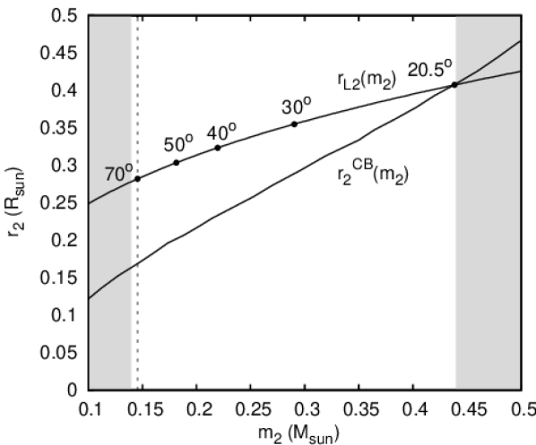
Figure 10: Size of the companion Roche Lobe (top curve) and ZAMS mass radius relation as from Chabrier & Baraffe (2000, bottom curve). The values taken by an assumed Roche Lobe filling companion star, for a set of inclinations and $m_{1}=1.4$, are also indicated. The left shaded region is excluded from the absence of eclipses, while the right shaded one from the assumption that the companion is not larger than its Roche Lobe. The minimum mass for $i<70^{\circ}$ is also plotted with a vertical dashed line.

The reflection continuum and the iron K$\alpha$ line we have modelled with a diskline indicate an inclination in the range 38–68^∘ (see Table 3 and Sec.5.3). This interval corresponds to $m_{2}=$0.15–0.23 for m${}_{1}=1.4$. Slightly larger values are found for heavier NS. The inclination estimate we have drawn from spectral fitting thus indicates that the companion is slightly bloated with respect to its ZAMS thermal equilibrium radius. A possible mechanism to drive a companion star out of thermal equilibrium is irradiation by the compact object, but to what extent it is important is still matter of debate (see Ritter, 2008, and references therein). However, irradiation is not strictly needed to account for the values we observe from IGR J17511–3057, as CV-like evolution can explain it if the companion star is slightly evolved at the onset of mass transfer (but still before the MS turn off), or heavier than 1 M_⊙. As Pylyser & Savonije (1989) shown, angular momentum losses driven by magnetic braking and gravitational radiation can still lead to a converging system (that is, a system that evolves decreasing its orbital period), even for slightly evolved, or heavy, companions. In these cases, the companion radius will be systematically larger than the ZAMS radius. To see this, we consider the evolutionary tracks calculated by Podsiadlowski et al. (2002). While an unevolved companion with initial mass of $m_{2}^{(i)}$=1 crosses the observed orbital period of IGR J17511–3057 when m${}_{2}\simeq 0.44$, as its radius is frozen to the ZAMS value, this happens for $m_{2}\simeq 0.16$ if it is slightly evolved, and thus larger, at the beginning of mass transfer. Similar results are obtained even for initially unevolved, but heavier, companion star (the evolutionary track for a $m_{2}^{(i)}=1.4$ companion star passes through the period of IGR J17511–3057 when $m_{2}=0.15$). Values of $m_{2}$ in agreement with the inclination indicated by spectral modelling can be thus obtained, for peculiar conditions of the companion star at the onset of mass transfer.

5.3 The X-ray spectrum

We presented in Sec.3.3 and 3.3 a detailed spectral analysis of the 0.5–200 keV X-ray emission of the AMSP IGR J17511–3057, using two different Comptonization models, and checking the presence reflection. The spectrum of IGR J17511–3057 is modelled by four components, (i) the accretion disc emission peaking at $\simeq 0.3$ keV; (ii) a $\simeq$ 0.6 keV blackbody of apparent radius $\simeq 7$ d₈ km; (iii) Comptonization from a hot ($kT_{e}\simeq 50$ keV) medium of moderate optical depth ($\tau\simeq 1.3$), of the thermal ($\simeq 1.3$ keV) photons provided by a $\simeq 3.5$ d₈ km region (iv) Compton reflection and an iron K$\alpha$ emission line, interpreted as coming from the accretion disc illuminated by the hard radiation emitted from the NS surface. The shape of the best fitting model does not change much using different Comptonization models. As the model PS-refl better addresses a number of physical aspects of this source emission (see Sec.3.3) we discuss the parameters thus obtained. Compton disc reflection is significantly detected regardless of the particular model used to describe Comptonization, as well as an iron line at an energy compatible with Fe XXV-XXVI. Even if reflection has not always been observed, such a spectral decomposition have already proved successful in the description of the X-ray spectrum AMSP (Gierliński et al. 2002, GP05, Falanga et al. 2005; Papitto et al. 2009; Patruno et al. 2009). In particular, the presence of disc thermal emission has always been detected when XMM-Newton high resolution spectra extending down to $\sim$1 keV were available. The similarities in the X-ray emission of AMSP can be viewed as an indication of how the physical processes that produce the bulk of their spectra are similar, and probably related to the presence of a magnetosphere in these systems.

The correlation between the energy dependence of the pulsed fraction and the spectral decomposition we have employed strongly suggests that the Comptonizing medium surrounds the hot spots on the NS surface. Gierliński et al. (2002), Poutanen & Gierliński (2003), GP05, Falanga et al. (2005) and Falanga et al. (2005) interpreted the similar hard components shown by other AMSPs as coming from Comptonization in a plasma heated in the accretion columns. The magnetic field collimates the in-falling matter in columns of radii that are few tenths of the NS size. Even for accretion rates $\sim 0.1$ $\dot{M}_{Edd}$ like those observed for these sources during outbursts, the local accretion rate $\dot{m}$ can therefore attain the Eddington level (Basko & Sunyaev, 1976). In such a case, the radiation pressure becomes comparable to the ram pressure of the plasma falling at supersonic velocities, and a shock may thus form, heating the electrons up to the observed large temperatures.

The observed $\simeq 0.6$ keV blackbody component is too cold to supply enough seed photons for the observed Comptonized spectrum. Disentangling the temperature of seed photons from that of the observed blackbody significantly improves the fit and ensure the energy balance between the hot plasma and the region that provides the seed photons. A similar result has already been obtained by GP05, modelling the X-ray spectrum of the AMSP, XTE J1751–305. The size of the region that provides the soft photons, $R_{soft}^{\infty}=3.4^{+0.1}_{-0.4}$ d₈ km, is compatible with the expected radius of an hot spot. The radius of the observed blackbody, $R_{BB}^{\infty}=6.3^{+0.3}_{-0.1}$ d₈ km, is instead of the same order of the asymptotic value taken by the radius of the thermal burst emission. This component is therefore emitted by a larger fraction of the NS surface.

The cooler thermal component can be safely attributed to the emission of an optically thick accretion disc. The contribution of this component at low energy is responsible for the decrease of the pulsed fraction. Moreover, the parameters we obtain with a diskbb model nicely fit the expectations for an accretion disc around an AMSP. Considering the range of inclinations indicated by the reflection component (38–68^∘), the model diskbb evaluates an apparent inner disc radius $R_{in}$ in the range 18–28 d₈ km. Such a radius is estimated approximating the disc temperature profile with its asymptotic behaviour $T(r)\propto r^{-3/4}$, without accounting for the decrease of the viscous torque at the inner boundary of the disc, and neglecting spectral hardening. To evaluate the importance of these effects we consider the disc model diskpn (Gierliński et al., 1999). The spectral shape found by diskbb is recovered after rescaling the inner disc radius $R_{in}$ by a factor $\approx 2.3$, for $m_{1}=1.4$, $d=8$kpc, $i=50^{\circ}$ and $f=1.7$, where f is the ratio between the colour and effective temperature (Shimura & Takahara, 1995). The inner radius indicated by disc emission modelling thus meets the request that an accretion disc around an X-ray pulsar is not truncated at radii much larger than the corotation radius, $R_{C}=(GM/4\pi^{2}\nu^{2})^{1/3}=42.8\>m_{1.4}$ km for IGR J17511–3057, where $m_{1.4}$ is the NS mass in units of 1.4 $M_{\odot}$. Also the ratio between the flux in the disc component and the total flux agrees with a truncation radius a few tens of km away from the NS star. From the virial theorem it is in fact expected that $F_{disc}/F_{tot}\simeq R_{*}/2r_{in}$. As we measure $F_{disc}/F_{tot}\simeq 0.1$, the flux ratio predicts $r_{in}\simeq 5R_{*}$, which substantially agrees with the measured value.

The presence of reflection features, such as an iron K$\alpha$ emission line and Compton reflection, is significantly detected in spectral fitting. The iron line stands at $\sim 4\sigma$ above the continuum and has an equivalent width of $\simeq 40$ eV. If modelled with a Gaussian, its width can only be constrained to be $\lower 2.15277pt\hbox{$\;\buildrel>\over{\sim}\;$}0.5$ keV. As the spectrum of this source is dominated by Comptonization in a hot and optically thin medium, it is hard to find alternatives to disc reflection in order to explain such a width. In the inner regions of the accretion disc the line is broadened and red-shifted by the effects of Keplerian motion and by the gravitational influence of the nearby NS. Modelling the feature with a diskline we obtain an estimate of the inner disc radius as $r_{in}=27^{+6}_{-9}$ R_g, which translates in $r_{in}=56^{+12}_{-19}$ km for a 1.4 M_⊙ NS. Even if it is rather loose due to the limited counting statistics, also this estimate overlaps with the corotation radius, as it is expected from accretion theories. The addition of the RXTE dataset to the XMM-Newton spectrum also allows the detection of the hump at $\sim 30$ keV expected from Compton reflection. The ionised state of the reflector is rather high, $\log\xi=3.0^{+0.4}_{-0.2}$. It is worth to note that the highly ionised surface in the reflector is in agreement with the transition energy of the broad iron line at E${}_{Fe}=6.82^{+0.09}_{-0.11}$ keV, that we identify as a Ly$\alpha$ resonant transition of Fe XXV (rest-frame energy at 6.70 keV), that is likely to be produced in a photo-ionised plasma at $\log\xi\simeq 3$ (Kallman et al., 2004). Considering the values indicated by the reflection continuum and by the iron line modelling, we give a conservative estimate of the inclination in the range 38–68^∘. Also the OVIII edge we find at a high absorption depth ($\tau=$0.1–0.3) can be tentatively interpreted in terms of disc reflection. As its width is $<34$ eV, the outer rings of the disc should be involved, in order to make the rotational broadening negligible.

5.4 The X-ray bursts

In Sec. 4 we have presented a spectral and temporal analysis of the bursts observed by XMM-Newton. Considering the Swift observations, Bozzo et al. (2010) concluded that the observed recurrence times could be reconciled with the persistent flux if it is assumed that the bursts are ignited in a pure helium environment.

This hypothesis can be checked estimating the local accretion rate $\dot{m}$ needed to produce the fluence of the second burst, which lags the first by $\Delta t=$40.9 ks. One has in fact that $\dot{m}=y/\Delta t$, where $y$ is the column depth at which the burst is ignited. The value of $y$ can be estimated as $y=4\pi d^{2}\mathcal{F}/Q_{nuc}R_{*}^{2}$ (see e.g. Galloway et al., 2008), where $\mathcal{F}=(1+z)\tau F_{peak}^{\infty}$ is the burst fluence, and $Q_{nuc}$ is the energy per nucleon released during the thermonuclear burning ($Q_{nuc}\approx 1.6$ MeV for complete burning of He into iron group elements,Wallace & Woosley 1981). The measured values (see Table 4) yield $y=(2.6\pm 0.6)\times 10^{8}$ d${}_{8}^{2}$ R${}_{10}^{-2}$ g cm^-2, and $\dot{m}=(6.3\pm 1.4)\times 10^{3}$ d${}_{8}^{2}$ R${}_{10}^{-2}$ g cm^-2 s${}^{-1}\simeq 0.08\;R_{10}^{-1}\dot{m}_{Edd}$, where $z=1.31$ is considered. This value of $\dot{m}$ agrees with the bolometric luminosity of the persistent emission. Assuming that the blackbody and the Comptonized component arise from the vicinity of the NS surface, and therefore the observed fluxes have to be corrected for general relativity effects, we in fact estimate from model PS-refl the persistent luminosity as, $L_{X}^{pers}=4\pi d^{2}[(1+z)^{2}(F_{BB}+F_{PS})+(F_{Disc}+F_{Refl})]=(1.6\pm 0.1)\times 10^{37}$ d${}_{8}^{2}$ erg s${}^{-1}\;\simeq 0.09$ m${}_{1.4}^{-1}$ L_Edd. The agreement between the persistent luminosity and the mass accretion rate needed to explain the bursts fluence and recurrence time, when it is assumed that all the hydrogen is steadily burnt between bursts, suggests that bursts are triggered in nearly pure helium environment. It is perhaps useful to clarify that the difference between the local accretion rate estimated by the burst properties, $\dot{m}\simeq 0.08\dot{m}_{Edd}$, and the rate needed for a shock to form in the accretion column, $\dot{m}\simeq\dot{m}_{Edd}$, arises as the first is evaluated averaging the accretion rate over the whole NS surface, while the latter considers only the column size. Such a treatment seems appropriate as a magnetic field $\lower 2.15277pt\hbox{$\;\buildrel<\over{\sim}\;$}10^{9}$ G like the one expected in an AMSP should be able to confine accreted matter in the polar caps up to a column density of $\simeq 10^{7}$ g cm^-2 (Brown & Bildsten, 1998), which is well below the value we measure. The accreted layer is therefore able to diffuse across the whole NS surface before the burst onset.

As no photospheric radius expansion is observed, an upper limit on the distance can be set as $d^{2}\lower 2.15277pt\hbox{$\;\buildrel<\over{\sim}\;$}{L_{PRE}}/{4\pi F_{peak}^{\infty}}$, where the luminosity at which photospheric radius expansion is expected, $L_{PRE}=(3.79\pm 0.15)\times 10^{38}$ erg s^-1, was empirically derived by Kuulkers et al. (2003). Considering the peak flux of the second burst and the associated uncertainty, we set an upper limit on the distance to the source of $10$ kpc at a 90% confidence level. The radius of the thermal emission attained during the burst decay can be identified with the NS radius, and used to put a reasonable lower limit on the distance to the source. The measured value $R_{app}=(7.0\pm 0.3)d_{8}$ km can be related to the effective radius through the relation, $R=R_{app}f_{C}^{2}(1+z)^{-1}$ (see e.g. Lewin et al., 1993). The factor $f_{C}$ takes into account spectral hardening, and has been estimated as $f_{C}\simeq 1.35$ by Madej et al. (2004), for the case of a source that does not reach the Eddington level. Solving the previous relation for $M>1.4$ M_⊙, and considering that a soft equation of state like the A predicts $R_{*}>8.5$ km and M$\lower 2.15277pt\hbox{$\;\buildrel<\over{\sim}\;$}1.92$ M_⊙ for a NS spinning at the rate of IGR J17511–3057 (Pandharipande, 1971; Cook et al., 1994), we obtain $d\lower 2.15277pt\hbox{$\;\buildrel>\over{\sim}\;$}6.5$ kpc, unless a strange star is considered. For a lighter NS (M=1.57 M_⊙) this limit increases to 6.9kpc. Given the estimated range of distances, it is possible to safely state that IGR J17511–3057 belongs to the Galactic bulge. Also the compatibility of the measured equivalent hydrogen absorption column with that observed from XTE J1751–305 (whose distance was estimated to be $\;\buildrel>\over{\sim}\;$ 7 kpc, Markwardt et al. 2002; Papitto et al. 2008) supports such a conclusion.

Pulsations are detected throughout the burst decay at a similar amplitude than that seen during the persistent emission, while during the first few seconds they disappear, probably because of the telemetry limitations of the EPIC-pn. Their phase is also compatible within 0.1–0.2 cycles with that of pre-burst pulsations, suggesting that magnetic channelling of accreted matter and the burst onset happen at a similar location on the NS surface. This indication is strengthened by the analysis performed by Riggio et al. (2010, submitted) over RXTE data. They find in fact that, with the exception of the first two seconds since the burst onset, the burst oscillations are phase locked to pre-burst pulsations within 0.1 cycle. Phase locking between burst and non-burst oscillations of an AMSP has already been observed by Watts et al. (2008), at a much larger accuracy ($\simeq$0.01 cycles) than that made available by the data presented here. As they discuss (see also references therein), the most appealing interpretation is in terms of the effect a temperature gradient between the fuel impact point on the surface, and the rest of the surface, may have on the ignition conditions, or on its development. A temperature gradient during the persistent emission is indeed indicated by our spectral modelling, which requires the region feeding the accretion columns of soft photons to be hotter than the rest of the surface. A firm explanation of the correlation between pulsations observed during bursts and during the persistent emission is anyway still missing.

References

- Altamirano et al. (2008) Altamirano D., Casella P., Patruno A., Wijnands R., van der Klis M., 2008, ApJ, 674, L45
- Anders & Grevesse (1989) Anders E., Grevesse N., 1989, Geochimica et Cosmochimica Acta, 53, 197
- Baldovin et al. (2009) Baldovin C., Kuulkers E., Ferrigno C., et al., 2009, ATel, 2196, 1
- Balucinska-Church & McCammon (1992) Balucinska-Church M., McCammon D., 1992, ApJ, 400, 699
- Basko & Sunyaev (1976) Basko M. M., Sunyaev R. A., 1976, MNRAS, 175, 395
- Bhattacharya & van den Heuvel (1991) Bhattacharya D., van den Heuvel E. P. J., 1991, Phys.Rep., 203, 1
- Boirin et al. (2005) Boirin L., Méndez M., Díaz Trigo M., Parmar A. N., Kaastra J. S., 2005, A&A, 436, 195
- Bozzo et al. (2010) Bozzo E., Ferrigno C., Falanga M., Campana S., Kennea J. A., Papitto A., 2010, A&A, 509, L3+
- Bradt et al. (1993) Bradt H. V., Rothschild R. E., Swank J. H., 1993, A&AS, 97, 355
- Brown & Bildsten (1998) Brown E. F., Bildsten L., 1998, ApJ, 496, 915
- Burderi et al. (2007) Burderi L., Di Salvo T., Lavagetto G., et al., 2007, ApJ, 657, 961
- Cackett et al. (2009) Cackett E. M., Altamirano D., Patruno A., Miller J. M., Reynolds M., Linares M., Wijnands R., 2009, ApJ, 694, L21
- Campana et al. (2003) Campana S., Ravasio M., Israel G. L., Mangano V., Belloni T., 2003, ApJ, 594, L39
- Casella et al. (2008) Casella P., Altamirano D., Patruno A., Wijnands R., van der Klis M., 2008, ApJ, 674, L41
- Chabrier & Baraffe (2000) Chabrier G., Baraffe I., 2000, A&AR, 38, 337
- Cook et al. (1994) Cook G. B., Shapiro S. L., Teukolsky S. A., 1994, ApJ, 422, 227
- Cui et al. (1998) Cui W., Morgan E. H., Titarchuk L. G., 1998, ApJ, 504, L27+
- D’Aì et al. (2010) D’Aì A., Di Salvo T., Ballantyne D., et al., 2010, A&A, in press (arXiv:1004.1963)
- D’Aì et al. (2009) D’Aì A., Iaria R., Di Salvo T., Matt G., Robba N. R., 2009, ApJ, 693, L1
- Fabian et al. (1989) Fabian A. C., Rees M. J., Stella L., White N. E., 1989, MNRAS, 238, 729
- Falanga et al. (2005) Falanga M., Bonnet-Bidaud J. M., Poutanen J., et al., 2005, A&A, 436, 647
- Falanga et al. (2005) Falanga M., Kuiper L., Poutanen J., et al., 2005, A&A, 444, 15
- Falanga et al. (2007) Falanga M., Soldi S., Shaw S., et al., 2007, ATel, 1046, 1
- Ford (2000) Ford E. C., 2000, ApJ, 535, L119
- Frank et al. (2002) Frank J., King A., Raine D. J., 2002, Accretion Power in Astrophysics: Third Edition. Cambridge, UK: Cambridge University Press, February 2002.
- Galloway et al. (2002) Galloway D. K., Chakrabarty D., Morgan E. H., Remillard R. A., 2002, ApJ, 576, L137
- Galloway et al. (2005) Galloway D. K., Markwardt C. B., Morgan E. H., Chakrabarty D., Strohmayer T. E., 2005, ApJ, 622, L45
- Galloway et al. (2007) Galloway D. K., Morgan E. H., Krauss M. I., Kaaret P., Chakrabarty D., 2007, ApJ, 654, L73
- Galloway et al. (2008) Galloway D. K., Muno M. P., Hartman J. M., Psaltis D., Chakrabarty D., 2008, ApJS, 179, 360
- Gierliński et al. (2002) Gierliński M., Done C., Barret D., 2002, MNRAS, 331, 141
- Gierliński & Poutanen (2005) Gierliński M., Poutanen J., 2005, MNRAS, 359, 1261
- Gierliński et al. (1999) Gierliński M., Zdziarski A. A., Poutanen J., Coppi P. S., Ebisawa K., Johnson W. N., 1999, MNRAS, 309, 496
- Grebenev et al. (2005) Grebenev S. A., Molkov S. V., Sunyaev R. A., 2005, ATel, 446, 1
- Hartman et al. (2008) Hartman J. M., Patruno A., Chakrabarty D., et al., 2008, ApJ, 675, 1468
- Iaria et al. (2009) Iaria R., D’Aí A., di Salvo T., Robba N. R., Riggio A., Papitto A., Burderi L., 2009, A&A, 505, 1143
- Jahoda et al. (2006) Jahoda K., Markwardt C. B., Radeva Y., Rots A. H., Stark M. J., Swank J. H., Strohmayer T. E., Zhang W., 2006, ApJS, 163, 401
- Kallman et al. (2004) Kallman T. R., Palmeri P., Bautista M. A., Mendoza C., Krolik J. H., 2004, ApJS, 155, 675
- Kuulkers et al. (2003) Kuulkers E., den Hartog P. R., in’t Zand J. J. M., Verbunt F. W. M., Harris W. E., Cocchi M., 2003, A&A, 399, 663
- Leahy et al. (2009) Leahy D. A., Morsink S. M., Chung Y., Chou Y., 2009, ApJ, 691, 1235
- Lewin et al. (1993) Lewin W. H. G., van Paradijs J., Taam R. E., 1993, Space Science Reviews, 62, 223
- Lightman & Zdziarski (1987) Lightman A. P., Zdziarski A. A., 1987, ApJ, 319, 643
- Madej et al. (2004) Madej J., Joss P. C., Różańska A., 2004, ApJ, 602, 904
- Magdziarz & Zdziarski (1995) Magdziarz P., Zdziarski A. A., 1995, MNRAS, 273, 837
- Markwardt et al. (2009) Markwardt C. B., Altamirano D., Strohmayer T. E., Swank J. H., 2009, ATel, 2237, 1
- Markwardt et al. (2009) Markwardt C. B., Altamirano D., Swank J. H., Strohmayer T. E., Linares M., Pereira D., 2009, ATel, 2197, 1
- Markwardt et al. (2002) Markwardt C. B., Swank J. H., Strohmayer T. E., in ’t Zand J. J. M., Marshall F. E., 2002, ApJ, 575, L21
- Nowak et al. (2009) Nowak M. A., Paizis A., Wilms J., et al., 2009, ATel, 2215, 1
- Paczyński (1971) Paczyński B., 1971, A&AR, 9, 183
- Pandharipande (1971) Pandharipande V. R., 1971, Nucl.Phys. A, 174, 641
- Papitto et al. (2007) Papitto A., di Salvo T., Burderi L., Menna M. T., Lavagetto G., Riggio A., 2007, MNRAS, 375, 971
- Papitto et al. (2009) Papitto A., Di Salvo T., D’Aì A., Iaria R., Burderi L., Riggio A., Menna M. T., Robba N. R., 2009, A&A, 493, L39
- Papitto et al. (2008) Papitto A., Menna M. T., Burderi L., di Salvo T., Riggio A., 2008, MNRAS, 383, 411
- Patruno et al. (2010) Patruno A., Altamirano D., Messenger C., 2010, MNRAS, pp 207–+
- Patruno et al. (2009) Patruno A., Hartman J. M., Wijnands R., Chakrabarty D., van der Klis M., 2009, arXiv:0902.4323
- Patruno et al. (2009) Patruno A., Rea N., Altamirano D., Linares M., Wijnands R., van der Klis M., 2009, MNRAS, 396, L51
- Podsiadlowski et al. (2002) Podsiadlowski P., Rappaport S., Pfahl E. D., 2002, ApJ, 565, 1107
- Poutanen (2006) Poutanen J., 2006, AdSpR, 38, 2697
- Poutanen & Beloborodov (2006) Poutanen J., Beloborodov A. M., 2006, MNRAS, 373, 836
- Poutanen & Gierliński (2003) Poutanen J., Gierliński M., 2003, MNRAS, 343, 1301
- Poutanen & Svensson (1996) Poutanen J., Svensson R., 1996, ApJ, 470, 249
- Protassov et al. (2002) Protassov R., van Dyk D. A., Connors A., Kashyap V. L., Siemiginowska A., 2002, ApJ, 571, 545
- Pylyser & Savonije (1989) Pylyser E. H. P., Savonije G. J., 1989, A&A, 208, 52
- Riggio et al. (2009) Riggio A., Papitto A., Burderi L., di Salvo T., D’Ai A., Iaria R., Menna M. T., 2009, ATel, 2221, 1
- Ritter (2008) Ritter H., 2008, New Astronomy Review, 51, 869
- Rothschild et al. (1998) Rothschild R. E., Blanco P. R., Gruber D. E., et al., 1998, ApJ, 496, 538
- Rybicki & Lightman (1979) Rybicki G. B., Lightman A. P., 1979, Radiative processes in astrophysics. New York, Wiley-Interscience, 1979. 393 p.
- Shimura & Takahara (1995) Shimura T., Takahara F., 1995, ApJ, 445, 780
- Stewart (2009) Stewart I. M., 2009, A&A, 495, 989
- Sunyaev & Titarchuk (1985) Sunyaev R. A., Titarchuk L. G., 1985, A&A, 143, 374
- van Paradijs & Lewin (1986) van Paradijs J., Lewin H. G., 1986, A&A, 157, L10
- Wallace & Woosley (1981) Wallace R. K., Woosley S. E., 1981, ApJS, 45, 389
- Watts et al. (2008) Watts A. L., Patruno A., van der Klis M., 2008, ApJ, 688, L37
- Watts et al. (2005) Watts A. L., Strohmayer T. E., Markwardt C. B., 2005, ApJ, 634, 547
- Weinberg et al. (2001) Weinberg N., Miller M. C., Lamb D. Q., 2001, ApJ, 546, 1098
- Wijnands & van der Klis (1998) Wijnands R., van der Klis M., 1998, Nat., 394, 344
- Yan et al. (1998) Yan M., Sadeghpour H. R., Dalgarno A., 1998, ApJ, 496, 1044
- Zdziarski et al. (1996) Zdziarski A. A., Johnson W. N., Magdziarz P., 1996, MNRAS, 283, 193
- Życki et al. (1999) Życki P. T., Done C., Smith D. A., 1999, MNRAS, 309, 561