Shear-driven and diffusive helicity fluxes in $\alpha\Omega$ dynamos

Abstract

We present nonlinear mean-field $\alpha\Omega$ dynamo simulations in spherical geometry with simplified profiles of kinematic $\alpha$ effect and shear. We take magnetic helicity evolution into account by solving a dynamical equation for the magnetic $\alpha$ effect. This gives a consistent description of the quenching mechanism in mean-field dynamo models. The main goal of this work is to explore the effects of this quenching mechanism in solar-like geometry, and in particular to investigate the role of magnetic helicity fluxes, specifically diffusive and Vishniac-Cho (VC) fluxes, at large magnetic Reynolds numbers ($R_{\rm m}$). For models with negative radial shear or positive latitudinal shear, the magnetic $\alpha$ effect has predominantly negative (positive) sign in the northern (southern) hemisphere. In the absence of fluxes, we find that the magnetic energy follows an $R_{\rm m}^{-1}$ dependence, as found in previous works. This catastrophic quenching is alleviated in models with diffusive magnetic helicity fluxes resulting in magnetic fields comparable to the equipartition value even for $R_{\rm m}=10^{7}$. On the other hand, models with a shear-driven Vishniac-Cho flux show an increase of the amplitude of the magnetic field with respect to models without fluxes, but only for $R_{\rm m}<10^{4}$. This is mainly a consequence of assuming a vacuum outside the Sun which cannot support a significant VC flux across the boundary. However, in contrast with the diffusive flux, the VC flux modifies the distribution of the magnetic field. In addition, if an ill-determined scaling factor in the expression for the VC flux is large enough, subcritical dynamo action is possible that is driven by the action of shear and the divergence of current helicity flux.

1 Introduction

A crucial point in the study of astrophysical dynamos is to understand the mechanism by which they saturate. Nevertheless, a consistent description of this process has rarely been considered in mean-field dynamo (MFD) modeling and only a heuristic description is often used. An important phenomenon happens when the dynamo operates in closed or periodic domains: the turbulent contribution to the dynamo equation, i.e., the $\alpha$ effect, decreases for large values of the magnetic Reynolds number. This process is known as catastrophic quenching and can pose a problem in explaining the generation of magnetic field in late type stars like the Sun or the Galaxy, where $R_{\rm m}$ could be of the order of $10^{9}$ or $10^{15}$, respectively.

In the last few years the nature of the catastrophic quenching has been identified as a consequence of magnetic helicity conservation (for a review see Brandenburg & Subramanian, 2005a). It has been found that in the nonlinear phase of the dynamo process, conservation of magnetic helicity gives rise to a magnetic $\alpha$ effect ($\alpha_{\rm M}$) with a sign opposite to the inductive contribution due to the helical motions, i.e., the kinematic $\alpha$ effect. As the production of $\alpha_{\rm M}$ depends on $R_{\rm m}$, the final value of the magnetic field should also follow the same dependence. However, real astrophysical bodies are not closed systems, but they have open boundaries that may allow a flux of magnetic helicity. The shedding of magnetic helicity may mitigate the catastrophic $\alpha$ quenching.

These ideas have been tested in direct numerical simulations (DNS) in both local Cartesian and global spherical domains. In the former (Brandenburg, 2005; , 2008) it has been clearly shown that open boundaries (e.g. vertical field boundary conditions) lead to a faster saturation of a large-scale magnetic field compared with cases in closed domains (perfect conductor or triple-periodic boundary conditions). In the latter, it has been found that it is possible to build up large-scale magnetic fields either with forced turbulence (Brandenburg, 2005; Mitra et al., 2010b) or with convectively driven turbulence (e.g., Brown et al., 2010; Käpylä et al., 2010). These models generally used vertical field boundary conditions.

In flux-transport dynamos (Dikpati & Charbonneau, 1999; , 2008) as well as in interface dynamos of the solar cycle (e.g. MacGregor & Charbonneau, 1997; Charbonneau & MacGregor, 1997) the quenching mechanism has been considered either through an ad hoc algebraic equation or by phenomenological considerations (Chatterjee, Nandy & Choudhuri, 2004), but most of the time the models do not consider the effects of magnetic helicity conservation. An exception is the recent paper by Chatterjee, Brandenburg & Guerrero (2010), where these effects have been considered in the context of an interface dynamo.

In general the magnetic helicity depends on time, so it is necessary to solve an additional dynamical equation for the contribution of the small-scale field to the magnetic helicity together with the induction equation for the magnetic field. In the past few years, some effort has already been made to consider this dynamical saturation mechanism in MFD models like in the 1D $\alpha^{2}$ dynamo models presented in Brandenburg, Candelaresi & Chatterjee (2009), in axisymmetric models in cylindrical geometry for the galactic $\alpha\Omega$ dynamo (Shukurov et al., 2006), and also in models with spherical geometry for an $\alpha^{2}$ dynamo (Brandenburg et al., 2007). The role of various kinds of magnetic helicity fluxes have been explored in several papers (Brandenburg, Candelaresi & Chatterjee, 2009; Zhang et al., 2006; Shukurov et al., 2006).

Our ultimate goal is to develop a self-consistent MFD model of the solar dynamo, with observed velocity profiles and turbulent dynamo coefficients computed from the DNS. This is a task that requires intensive efforts. Hence we shall proceed step by step, starting with simple models and then including more realistic physics on the way. In this work we will study the effects of magnetic helicity conservation in simplified $\alpha\Omega$ dynamo models for a considerable number of cases. More importantly, we shall perform our calculations in spherical geometry, which is appropriate for describing stellar dynamos, with suitable boundary conditions, and considering shear profiles which are a simplified version of the observed solar differential rotation. We shall also explore how magnetic helicity fluxes affect the properties of the solution. Two classes of fluxes are considered in this paper: a diffusive flux and a shear-driven or Vishniac-Cho (hereafter VC) flux (Vishniac & Cho, 2001). We consider models with either radial or latitudinal shear. The effects of meridional circulation will be investigated in detail in a companion paper (Chatterjee, Guerrero & Brandenburg, 2010).

This paper is organized as follows: in Section 2 we describe the basic mathematical formalism of the $\alpha\Omega$ dynamo, give the formulation of the equation for $\alpha_{\rm M}$ and also justify the fluxes included. In Section 3 we describe the numerical method and then, we present our results in Section 4 starting from a dynamo model with algebraic quenching to models with dynamical $\alpha$ quenching and different fluxes. Finally, we provide a summary of this work in Section 5.

2 The $\alpha\Omega$ dynamo model

In mean-field dynamo theory, the evolution of the magnetic field is described by the mean-field induction equation,

$$\frac{\partial\overline{\bm{B}}}{\partial t}=\bm{\nabla}\times\left(\overline{\bm{U}}\times\bm{\overline{B}}+\bm{\overline{\cal{E}}}-\eta_{\rm m}\bm{\nabla}\times\bm{\overline{B}}\right),$$ (1)

where $\bm{\overline{B}}$ and $\bm{\overline{U}}$ represent the mean magnetic and velocity fields, respectively, $\eta_{\rm m}$ is the molecular diffusivity, $\bm{\overline{\cal{E}}}=\alpha\bm{\overline{B}}-\eta_{\rm t}\mu_{0}\bm{\overline{J}}$ is the mean electromotive force obtained using a closure theory like the first order smoothing approximation, where $\bm{\overline{\cal{E}}}$ gives the contribution of the small-scale components on the large-scale field, $\alpha$ is the non-diffusive contribution of the turbulence, $\eta_{\rm t}$ is the turbulent magnetic diffusivity, $\bm{\overline{J}}=\bm{\nabla}\times\bm{\overline{B}}/\mu_{0}$ is the mean current density, and $\mu_{0}$ is the vacuum permeability.

In spherical coordinates and under the assumption of axisymmetry, it is possible to split the magnetic and the velocity fields into their azimuthal and poloidal components, $\bm{\overline{B}}=B\bm{\hat{e}}_{\phi}+\bm{\nabla}\times(A\bm{\hat{e}}_{\phi})$ and $\bm{\overline{U}}=r\sin\theta\Omega\bm{\hat{e}}_{\phi}+\bm{u}_{\rm p}$, respectively. For the sake of simplicity we shall not consider the meridional component of the flow, i.e. ${\bm{u}}_{\rm p}=0$. Then, the toroidal and poloidal components of equation (1) may be written as

$$\frac{\partial B}{\partial t} \!=\! s{\bm{B}}_{\rm p}\cdot\bm{\nabla}\Omega-\left[\bm{\nabla}\eta\times(\bm{\nabla}\times B\bm{\hat{e}}_{\phi})\right]_{\phi}+\eta D^{2}B\;,\quad,$$ (2)

$$\frac{\partial A}{\partial t} \!=\! \alpha B+\eta D^{2}A\;,$$ (3)

where $D^{2}=\nabla^{2}-s^{-2}$ is the diffusion operator, $\eta=\eta_{\rm m}+\eta_{\rm t}$, $s=r\sin\theta$ is the distance from the axis, and $\bm{B}_{\rm p}=\bm{\nabla}\times(A\hat{e}_{\phi})$ is the poloidal field.

The two source terms in equations (2) and (3), $s\bm{B}_{\rm p}\cdot\bm{\nabla}\Omega$ and $\alpha B$, express the inductive effects of shear and turbulence, respectively. The relative importance of these two effects may be quantified through the non-dimensional dynamo numbers: $C_{\Omega}=\Delta\Omega L^{2}/\eta_{\rm t}$ and $C_{\alpha}=\alpha_{0}L/\eta_{\rm t}$, where $\Delta\Omega$ is the angular velocity different between top and bottom of the domain. Note that equations (2) and (3) are valid only in the limit $C_{\Omega}\gg C_{\alpha}$, known as $\alpha\Omega$ dynamo.

The inductive effects of the shear may be understood as the stretching of the magnetic field lines due to the change in the angular velocity between two adjacent points. On the other hand, the kinematic $\alpha$-effect is the consequence of helical motions of the plasma which produce screw-like motions in the rising blobs of the magnetic field. Using the first order smoothing approximation it may be expressed as:

$$\alpha_{\rm K}=-\textstyle{\frac{1}{3}}\tau\overline{\bm{\omega}\cdot\bm{u}}\;,$$ (4)

where, $\tau$ is the correlation time of the turbulent motions and $\bm{\omega}=\bm{\nabla}\times\bm{u}$ is the small-scale vorticity. The saturation value of the magnetic field may be obtained by multiplying $\alpha_{\rm K}$ by the quenching function $f_{\rm q}=\left(1+B^{2}/B_{\rm eq}^{2}\right)^{-1}$, which saturates the exponential growth of the magnetic field at values close to the equipartition field strength given by $B_{\rm eq}=(\mu_{0}\overline{\rho{\bm{u}}^{2}})$. This form of algebraic quenching was introduced heuristically (see, e.g. , 1972) and has been often used as the standard quenching mechanism in many dynamo simulations. However, it does not give information about the back reaction process and is independent of any parameter of the system like the magnetic Reynolds number. A consistent description of the quenching mechanism will be presented in the following section.

2.1 Dynamical $\alpha$ effect

Recently, it has been demonstrated that when the amplitude of the magnetic field reaches values near the equipartition, the $\alpha$-effect is modified by a magnetic contribution, the so called magnetic $\alpha$ effect, denoted by $\alpha_{\rm M}$. It is usually the case that $\alpha_{\rm M}$ has a sign opposite to $\alpha_{\rm K}$ resulting thus in the saturation of the magnetic field. Pouquet, Frisch & Léorat (1976) have shown that $\alpha_{\rm M}$ is proportional to the small-scale current helicity of the system, hence it is possible to write $\alpha$ as a sum of two contributions, one from the fluid turbulence and other from the magnetic field, as follows:

$$\alpha=\alpha_{\rm K}+\alpha_{\rm M}=-{\textstyle\frac{1}{3}}\tau\overline{\bm{\omega}\cdot\bm{u}}+\textstyle{\frac{1}{3}}\tau\overline{\bm{j}\cdot\bm{b}}/\overline{\rho}\;,$$ (5)

where $\overline{\rho}$ is the mean density of the medium, assumed here as a constant, and $\bm{j}=\bm{\nabla}\times\bm{b}/\mu_{0}$ is the current density of the fluctuating field. The mathematical expression that describes the evolution of $\alpha_{\rm M}$ may be obtained by taking into account the magnetic helicity evolution (Blackman & Brandenburg, 2002), which leads to:

$$\frac{\partial\alpha_{\rm M}}{\partial t}=-2\eta_{\rm t}k_{\rm f}^{2}\left(\frac{\bm{\overline{\cal{E}}}\cdot\overline{{\bm{B}}}}{B_{\rm eq}^{2}}+\frac{\alpha_{\rm M}}{R_{\rm m}}\right)-\bm{\nabla}\cdot\bm{\overline{{\cal{F}}}}_{\alpha}\;,$$ (6)

where $k_{\rm f}=2\pi/(L-r_{c})$ with $r_{c}=0.7L_{0}$ is a suitable choice for the wave number of the forcing scale, the magnetic Reynolds number $R_{\rm M}=\eta_{\rm t}/\eta_{\rm m}$ and $\bm{\overline{\cal{F}}}_{\alpha}$ is the flux of the magnetic $\alpha$ effect related to the flux of the small-scale magnetic helicity, $\bm{\overline{F}}_{\rm f}$ through:

$$\bm{\overline{\cal F}}_{\alpha}=\frac{\mu_{0}\overline{\rho}\eta_{\rm t}k_{\rm f}^{2}}{B_{\rm eq}^{2}}\bm{\overline{F}}_{\rm f}\quad,$$ (7)

According to previous authors $\alpha_{\rm M}$ has a finite value in the interior of the domain in absence of fluxes ($\bm{\overline{\cal{F}}}_{\alpha}=0$), and its sign is usually opposite to the sign of $\alpha_{\rm K}$ in such a way that the final amplitude of the total $\alpha$-effect decreases, and so does the final value of the magnetic energy.

2.2 Magnetic helicity fluxes

Recently it has been pointed out that the catastrophic quenching could be alleviated by allowing the flux of small-scale magnetic (or current) helicity out of the domain, so that the total magnetic helicity inside need not be conserved any longer. Alternately, we may introduce those fluxes in the equation for $\alpha_{\rm M}$; see equation (7). Several candidates have been proposed for the helicity fluxes in the past (Kleeorin & Rogachevskii, 1999; Vishniac & Cho, 2001; Subramanian & Brandenburg, 2004). Amongst them are the flux of magnetic helicity across the iso-rotation contours, advective and diffusive fluxes and also the explicit removal of magnetic helicity in processes like coronal mass ejections or galactic fountain flows, for the case of the galactic dynamo.

From the mathematical point of view, the nature of the flux terms in the equation for $\alpha_{\rm M}$ has not been demonstrated with sufficient rigor. However, several DNS have pointed to its existence.

Firstly, the shearing box convection simulations of (2008) showed that in the presence of open boundaries, the large-scale magnetic field grows on temporal scales much shorter than the dissipative time scale. They concluded from this that open boundaries may allow the magnetic helicity to escape out of the system. These experiments seem to be compatible with the flux proposed by Vishniac & Cho (2001), whose functional form may be expressed as (see Subramanian & Brandenburg, 2004; Brandenburg & Subramanian, 2005b, for further details):

$$\overline{\cal F}^{\rm VC}_{i}=C_{\rm VC}\epsilon_{ijl}\overline{\mathsf{S}}_{lk}\overline{B}_{j}\overline{B}_{k}\quad,$$ (8)

where $\overline{\mathsf{S}}_{lk}=\frac{1}{2}(\overline{U}_{l,k}+\overline{U}_{k,l})$ is the mean rate of strain tensor and $C_{\rm VC}$ is a non-dimensional scaling factor. As we assume ${\bm{u}}_{\rm p}=0$, this flux has the following three components:

$$\overline{\cal F}^{\rm VC}_{r} = C_{\rm VC}\left[\overline{\mathsf{S}}_{\phi r}B_{\theta}B_{\rm r}+\overline{\mathsf{S}}_{\theta\phi}(B_{\theta}^{2}-B_{\phi}^{2})\right]\;,$$ (9)

$$\overline{\cal F}^{\rm VC}_{\theta} = C_{\rm VC}\left[-\overline{\mathsf{S}}_{\phi\theta}B_{r}B_{\theta}+\overline{\mathsf{S}}_{r\phi}(B_{\phi}^{2}-B_{r}^{2})\right]\;,$$ (10)

$$\overline{\cal F}^{\rm VC}_{\phi} = C_{\rm VC}\left[\overline{\mathsf{S}}_{\theta\phi}B_{r}B_{\phi}-\overline{\mathsf{S}}_{r\phi}(B_{\theta}^{2}-B_{\phi}^{2})\right]\;,$$ (11)

with $\overline{\mathsf{S}}_{\phi r}=\overline{\mathsf{S}}_{r\phi}=r\sin\theta(\partial\Omega/\partial r)/2$ and $\overline{\mathsf{S}}_{\theta\phi}=\overline{\mathsf{S}}_{\phi\theta}=\sin\theta(\partial\Omega/\partial\theta)/2$.

Secondly, Mitra et al. (2010a) performed $\alpha^{2}$ dynamo simulations driven by forced turbulence in a box with an equator. They found that the diffusive flux of $\alpha_{\rm M}$ across the equator can be fitted to a Fickian diffusion law given by,

$$\mbox{\boldmath${\cal F}$}_{\rm D}=-\kappa_{\alpha}(r)\bm{\nabla}\alpha_{\rm M}\;.$$ (12)

They also computed the numerical value of this diffusion coefficient, and found it to be of the order of turbulent diffusion coefficient. They also found that the time averaged flux is gauge independent. Both results were later corroborated by simulations without equator, but with a decline of kinetic helicity toward the boundaries (, 2010).

Additionally, magnetic helicity may be advected by the mean velocity with a flux given by $\bm{\overline{\cal F}}_{\rm ad}=\alpha_{\rm M}\overline{\bm{U}}$, or it may be expelled from the solar interior by coronal mass ejections (CMEs) or by the solar wind. This flux, ${\cal F}_{\rm CME}$, may account for $\sim 10$% of the total helicity generated by the solar differential rotation, as estimated by Berger & Ruzmaikin (2000). It can be modeled by artificially removing a small amount of $\alpha_{\rm M}$ every $\tau$ time (Brandenburg, Candelaresi & Chatterjee, 2009), or also by a radial velocity field that mimics the solar wind.

The total flux of magnetic helicity may be written as the sum of these contributions,

$$\bm{\overline{\cal F}}=\bm{\overline{\cal F}_{\rm VC}}+\bm{\overline{\cal F}}_{\rm D}+\bm{\overline{\cal F}}_{\rm ad}+\bm{\overline{\cal F}}_{\rm CME}\;.$$ (13)

Since in this dynamo model we do not include any component of the velocity field other than the differential rotation, in this study we will consider only the first two terms on the rhs of equation (13).

3 The model

We solve equation (2), (3) and (6) for $A$, $B$ and $\alpha_{\rm M}$ in the meridional plane in the range $0.6L\leq r\leq L$ and $0\leq\theta\leq\pi$. We consider two different layers inside the spherical shell. In the inner one the dynamo production terms are zero and go smoothly to a finite value in the external layer. The magnetic diffusivity changes from a molecular to a turbulent value from the bottom to the top of the domain. This is achieved by considering error function profiles for the magnetic diffusivity, the differential rotation, and the kinetic $\alpha$ effect, respectively (see Fig. 1):

$$\eta(r) = \eta_{\rm m}+\eta_{\rm t}\Theta(r,r_{1},w_{1})\;,$$ (14)

$$\frac{\partial\Omega}{\partial r}(r) = C_{\Omega}\left(\frac{L^{2}}{\eta_{\rm t}}\right)\Theta(r,r_{2},w_{1})\;,$$ (15)

$$\alpha_{\rm K}(r,\theta) = C_{\alpha}\left(\frac{L}{\eta_{\rm t}}\right)\Theta(r,r_{1},w_{1})\cos\theta\;,$$ (16)

where $\Theta(r,r_{1,2},w)=\frac{1}{2}\left[1+\mathrm{erf}\left\{(r-r_{1,2})/{w_{1}}\right\}\right]$, with $r_{1}=0.7L_{0}$, $r_{2}=0.72L_{0}$ and $w_{1}=0.025L_{0}$. We fix $C_{\Omega}=-10^{4}$ and vary $C_{\alpha}$.

The boundary conditions are chosen as follows: at the poles, $\theta=0,\pi$, we impose $A=B=0$; at the base of the domain, we impose a perfect conductor boundary condition, i.e. $A=\partial(rB)/\partial r=0$. Unless noted otherwise, we use at the top a vacuum condition by coupling the magnetic field inside with an external potential field, i.e., $(\nabla^{2}-s^{-2})A=0$. A good description of the numerical implementation of this boundary condition may be found in Dikpati & Choudhuri (1994).

The equations for $A$ and $B$ are solved using a second-order Lax-Wendroff scheme for the first derivatives, and centered finite differences for the second-order derivatives. The temporal evolution is computed by using a modified version of the ADI method of Peaceman & Rachford (1955) as explained in Dikpati & Charbonneau (1999). This numerical scheme has been used previously in several works on the flux-transport dynamo and the results were found to be in good agreement with those using other numerical techniques (, 2007, 2008; , 2009).

In the absence of magnetic helicity fluxes, equation (6) for $\alpha_{\rm M}$ corresponds to an initial value problem that can be computed explicitly. However, as we are going to include a diffusive flux, we use for $\alpha_{\rm M}$ the same numerical technique used for $A$ and $B$. All the source terms on the right hand side of equation (6) are computed explicitly. We have tested the convergence of the solution for $64^{2}$, $128^{2}$, and $256^{2}$ grid points. For cases with small $R_{\rm m}$, there are no significant differences between different resolutions, but for high $R_{\rm m}$, $64^{2}$ grid points is insufficient to properly resolve the sharp diffusivity gradient. A resolution of $128^{2}$ grid points is a good compromise between accuracy and speed.

Figure 1: Profiles of the dynamo ingredients, $\alpha_{\rm K}$ (solid line), $\partial\Omega/\partial r$ (dashed line) and $\eta_{\rm t}$ (dot-dashed line). All the values are normalized to their maximum value.

4 Results

4.1 $\alpha\Omega$ dynamos with algebraic quenching

Table 1: Summary of main parameters and results of the numerical simulations.

Run	$C_{\alpha}$	$R_{\rm m}$	$\kappa_{\alpha}$ ($\eta_{\rm t}$)	$C_{\rm VC}$	$\overline{\bm{B}}_{\rm rms}/B_{\rm eq}$	$T(L_{0}^{2}/\eta_{\rm t})$	$t$ ($L_{0}^{2}/\eta_{\rm t}$)
CaC	1.975	$10$	-	-	0.0008	0.0486	$1.0$
Ca2.0	2.0	$10$	-	-	0.15	0.0484	$1.0$
Ca2.1	2.1	$10$	-	-	0.33	0.0477	$3.0$
Ca2.2	2.2	$10$	-	-	0.45	0.0471	$3.0$
Ca2.3	2.3	$10$	-	-	0.56	0.0464	$3.0$
Ca2.4	2.4	$10$	-	-	0.64	0.0460	$3.0$
Ca2.5	2.5	$10$	-	-	0.69	0.0455	$3.0$
Rm10	2.5	$10$	-	-	0.21	0.0422	$4.0$
Rm50	2.5	$50$	-	-	0.25	0.0446	$4.0$
Rm1e2	2.5	$100$	-	-	0.2	0.0455	$4.0$
Rm1e3	2.5	$10^{3}$	-	-	0.07	0.0464	$4.0$
Rm2e3	2.5	$2$$\times$$10^{3}$	-	-	0.05	0.0464	$6.0$
Rm5e3	2.5	$5$$\times$$10^{3}$	-	-	0.03	0.0468	$15.0$
Rm1e4	2.5	$10^{4}$	-	-	0.02	0.048	$15.0$
DRm10	2.5	$10$	$0.005$	-	0.22	0.0422	$4.0$
DRm50	2.5	$50$	$0.005$	-	0.26	0.0446	$4.0$
DRm1e2	2.5	$100$	$0.005$	-	0.20	0.0455	$4.0$
DRm1e3	2.5	$10^{3}$	$0.005$	-	0.09	0.0460	$4.0$
DRm1e4	2.5	$10^{4}$	$0.005$	-	0.06	0.0457	$5.0$
DRm1e5	2.5	$10^{5}$	$0.005$	-	0.05	0.0460	$7.0$
DRm1e6	2.5	$10^{6}$	$0.005$	-	0.05	0.0457	$8.0$
DRm1e7a	2.5	$10^{7}$	$0.001$	-	0.026	0.0457	$20.0$
DRm1e7b	2.5	$10^{7}$	$0.005$	-	0.05	0.0460	$10.0$
DRm1e7c	2.5	$10^{7}$	$0.01$	-	0.073	0.0460	$10.0$
DRm1e7d	2.5	$10^{7}$	$0.03$	-	0.12	0.0460	$8.0$
DRm1e7e	2.5	$10^{7}$	$0.05$	-	0.15	0.0457	$4.0$
DRm1e7f	2.5	$10^{7}$	$0.1$	-	0.20	0.0460	$4.0$
DRm1e7g	2.5	$10^{7}$	$1.0$	-	0.54	0.0458	$4.0$
DRm1e7h	2.5	$10^{7}$	$5.0$	-	1.23	0.060	$4.0$
DRm1e7i	2.5	$10^{7}$	$10.0$	-	1.76	0.0457	$4.0$
VCa	2.5	$10^{3}$	-	0.002	0.032	0.0449	$4.0$
VCb	2.5	$10^{3}$	-	0.01	0.02	0.0442	$4.0$
VCc	2.5	$10^{3}$	-	-0.002	0.02	0.0447	$4.0$
VCd	2.5	$10^{4}$	-	-0.002	-	-	$4.0$
VCD	2.5	$10^{3}$	$0.1$	0.001	0.11	0.0446	$4.0$
Re1e3θ	2.5	$10^{3}$	-	-	0.023	0.0282	$8.0$
VCθa	2.5	$10^{3}$	-	0.004	0.04	0.033	$4.0$
VCDθ	2.5	$10^{3}$	0.1	0.004	0.062	0.0266	$4.0$
Re1e3θvf	2.5	$10^{3}$	-	-	0.036	0.032	$6.0$
VCθvf	2.5	$10^{3}$	-	0.004	0.075	0.033	$6.0$

In order to characterize our $\alpha\Omega$ dynamo model we start by exploring the properties of the system when the saturation is controlled by algebraic quenching with $f_{q}=(1+B^{2}/B_{\rm eq}^{2})^{-1}$. We found that, with the profiles given by equations (14)–(16), Fig. 1, the critical dynamo number is around $2\times 10^{4}$ (i.e., $C_{\alpha}^{\rm C}=1.975$). The solution for the model is a dynamo wave traveling towards the equator since it obeys the Parker-Yoshimura sign rule (see Fig. 2). In this case, the maximum amplitude of the magnetic field depends only on the dynamo number of the system, $C_{\alpha}C_{\Omega}$, as can be seen in the bifurcation diagram in Fig. 3. The quenching formula is here independent of $R_{\rm m}$, so the saturation amplitude is also independent on $R_{\rm m}$.

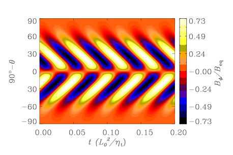
Figure 2: Time-latitude butterfly diagram for the toroidal component of the magnetic field at $r=0.72L_{0}$, for an $\alpha\Omega$ dynamo model with $C_{\Omega}=-10^{4}$ and $C_{\alpha}=2.5$.

Figure 3: Magnetic field average amplitude as a function of $C_{\alpha}$ using an algebraic quenching function that is independent of $R_{\rm m}$.

4.2 $\alpha\Omega$ dynamos with dynamical quenching

In this section we consider dynamo saturation through the dynamical equation for $\alpha_{\rm M}$ described in Section 2.1. In this models we distinguish three different stages in the time evolution of the magnetic field: a growing phase, a saturation phase and a final relaxation stage (see panels a, b and c of Fig. 5). The magnetic field is amplified from its initial value, $5\times 10^{-4}B_{\rm eq}$, following an exponential growth. From the earliest stages of the evolution we notice the growth of $\alpha_{\rm M}$ with values that are predominantly negative in the northern hemisphere and positive in the southern hemisphere. The latitudinal distribution of $\alpha_{\rm M}$ is fairly uniform in the active dynamo region, spanning from the equator to $\sim 60^{\circ}$ latitude. The radial distribution exhibits two narrow layers where the sign of $\alpha_{\rm M}$ is opposite to the dominant one developing at each hemisphere. These are located at the base of the dynamo region ($r\sim 0.7L_{0}$) and at a thin layer near to the surface ($r>0.95$). In the equation for the magnetic $\alpha$ effect, equation (6), the production term is proportional to $\bm{\overline{\cal{E}}}\cdot\overline{\bm{B}}=\alpha\overline{\bm{B}}^{2}-\eta_{\rm t}\mu_{0}\bm{\overline{J}}\cdot\overline{\bm{B}}$. The first component of this term has the same sign as $\alpha_{\rm K}$, which in general is positive in the northern and negative in the southern part of the domain. The minus sign in front of the right hand side of equation (6) defines then the sign of $\alpha_{\rm M}$. However, at the base and at the top of the dynamo region, $\alpha_{\rm K}\rightarrow 0$ and $B\rightarrow 0$, respectively. The term $\eta_{\rm t}\bm{\overline{J}}\cdot\bm{\overline{B}}$ is the only source of $\alpha_{\rm M}$ and leads to the formation of these two thin layers.

The space-time evolution of $\alpha_{\rm M}$ depends on the value of the magnetic Reynolds number. For small $R_{\rm m}$, the decay term in equation 6 (i.e. the second term in the parenthesis) becomes important, so that there is a competition between the production and decay terms resulting in an oscillatory behavior in the amplitude of the magnetic $\alpha$ effect, as is indicated by the vertical bars in the middle panel of Fig. 7. The period of these oscillations is the half the period of the magnetic cycle. With increasing $R_{\rm m}$, the amplitude of the oscillations decreases such that for $R_{\rm m}\leq 10^{3}$, $\alpha_{\rm M}$ is almost steady.

The morphology of the magnetic field corresponds to a multi-lobed pattern of alternating polarity (left panels of Fig. 5). These lobes are radially distributed in the whole dynamo region with maximum amplitude at the base of this layer. The poloidal magnetic field follows a similar pattern with lines that are open at the top of the domain due to the potential field boundary condition. There is a phase shift between toroidal and poloidal components which we have estimated to be $\sim 0.4\pi$. The model preserves the initial dipolar parity during the entire evolution.

The evolution of $\alpha_{\rm M}$ traces the growth of the magnetic field, but its final value depends on the magnetic Reynolds number. For small $R_{\rm m}$, after saturation, $\alpha_{\rm M}$ reaches a steady state, but for large $R_{\rm m}$, its relaxation is modulated by over-damped oscillations. The relaxation time is proportional to $R_{\rm m}$, which means that for $R_{\rm m}\gg 1$ the simulation must run for many diffusion times. The differences in the relaxation time observed for $\alpha_{\rm M}$ reflects the evolution of the magnetic field, as is shown in Fig. 4.

We observe that the rms value of the magnetic field remains steady during the saturation phase for $R_{\rm m}<10^{2}$. For $10^{2}<R_{\rm m}<10^{3}$, a bump appears in the curve of magnetic field evolution, followed by the relaxation to a steady value, whereas for $R_{\rm m}>10^{3}$, the magnetic energy shows over-damped relaxations with a final energy proportional to $\rm{Rm}^{-1}$ as has been previously reported (Brandenburg et al., 2007). These oscillations in the time evolution plot of the averaged magnetic field have been reported in mean field dynamo simulations including the dynamical $\alpha$-effect (Brandenburg & Subramanian, 2005b).

Not many DNS of $\alpha\Omega$ dynamo exist so far in the literature with $R_{\rm m}\geq 100$ in order to compare with our results. However, in the local $\alpha\Omega$ dynamo simulations of (2008), a rapid decay of the magnetic field seems to occur after the initial saturation for moderate values of $R_{\rm m}$. This decay forms a bump in the curve of the averaged magnetic field (see their Fig. 14), similar to the bump that we obtain for $10^{2}<R_{\rm m}<10^{3}$.

For reasons of clarity in the Fig. 4 we do not show the entire time evolution of each simulation with $R_{\rm m}>10^{3}$. The total evolution time as well as the final value of the magnetic field of each simulation are shown in the Table 1. For magnetic Reynolds numbers above $2\times 10^{4}$, the initial kinematic phase is followed by a decay phase during which the total $\alpha$ effect goes through subcritical values and then the dynamo fails to start again.

In Fig. 5 we present the meridional distribution of the magnetic field (left panel), $\alpha_{\rm M}$ (middle panel) and the total $\alpha$ (right panel), in normalized units, for the three different stages of evolution corresponding to the early kinematic phase, the late kinematic phase and the saturated phase. These snapshots correspond to the simulation with $R_{\rm m}=10^{3}$ (Run Rm1e3 in Table 1). The multi-lobed pattern of the toroidal field represented with filled contours remains unchanged during the evolution even though its amplitude increases. The same occurs for the poloidal component, shown by continuous and dashed streamlines for positive and negative values, respectively.

The magnetic $\alpha$ effect (middle panels) is formed first at latitudes between $\pm 30^{\circ}$ and then it amplifies and expands to latitudes up to $\sim\pm 60^{\circ}$. This makes the total $\alpha$ effect, initially similar to $\alpha_{\rm K}$ (Fig. 1 and top panel of Fig. 5a), smaller at lower latitudes in the central area of the dynamo region. At the bottom and at the top of the domain $\alpha_{\rm M}$ and $\alpha_{\rm K}$ have the same sign making the total $\alpha$ larger. However, the global effect is a decrease of the dynamo efficiency.

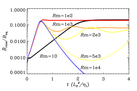
Figure 4: Time evolution of the averaged mean magnetic field for different values of $R_{\rm m}$. Note that for $R_{\rm m}>10^{3}$, we have allowed the simulations to evolve more than $4$ diffusion times, as indicated in Table 1.

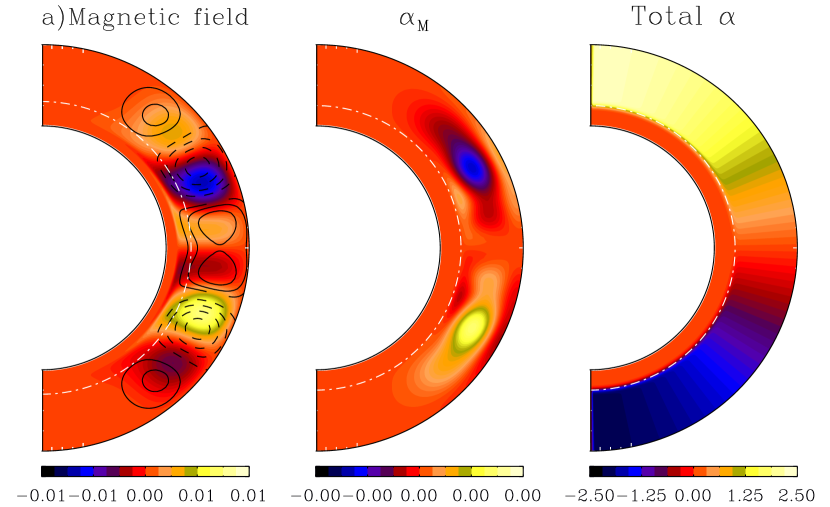
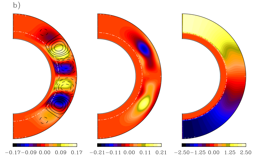
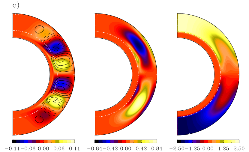
Figure 5: Meridional snapshots of three different phases of evolution of the dynamo model with dynamical quenching, a) $t=0.25$ ($L_{0}^{2}/\eta_{\rm t}$), b) $t=0.5$ ($L_{0}^{2}/\eta_{\rm t}$) and c) $t=2.0$ ($L_{0}^{2}/\eta_{\rm t}$). The left panel shows the contours of toroidal magnetic field in color scale, and positive (negative) poloidal magnetic field lines in continuous (dashed) lines. The central panel shows the distribution of $\alpha_{\rm M}$, and the right panel shows the distribution of the residual $\alpha$. All values are in non-dimensional units (i.e., $\overline{\bm{B}}/B_{\rm eq}$), so that the color scale is different for each figure as indicated in the respective color bar.

4.3 Diffusive flux for $\alpha_{\rm M}$

In this section we consider a Fickian diffusion term in equation (12) for $\alpha_{\rm M}$. We consider a diffusion coefficient varying from $5\times 10^{-3}\eta_{\rm t}$ to $10\,\eta_{\rm t}$ in the dynamo region and with $\kappa_{\alpha}=\eta_{\rm m}$ in the bottom layer. In these cases, the initial evolution of $\alpha_{\rm M}$ is similar to the cases presented in the previous section: negative (positive) values for $\alpha_{\rm M}$ in the northern (southern) hemisphere, with narrow regions of opposite values nearby the regions where $\alpha_{\rm K}=0$ or ${\bm{B}}=0$. However, at the later stages, $\alpha_{\rm M}$ is much more diffuse in the entire domain and has only one sign in each hemisphere. This is the result of cancellation of $\alpha_{\rm M}$ with opposite signs occurring in each hemisphere due to radial diffusion. Contrary to the cases without fluxes, we now obtain finite values of $B_{\rm sat}$ for large values of $R_{\rm m}$, as can be seen in Fig. 6. All the cases depicted in this figure correspond to $\kappa_{\alpha}=0.005\eta_{\rm t}$. We notice that the final value of the magnetic field still remains small compared to the equipartition ($\leq 0.1B_{\rm eq}$), but it is clear that even this very modest diffusion prevents the $\alpha$ effect from being catastrophically quenched. This is also evident from the top panel of Fig. 7, where we plot the final strength of $\overline{\bm{B}}$ as a function of $R_{\rm m}$, for the cases with and without dissipative flux. In the middle and bottom panels of the Fig. 7 we compare the behavior of the normalized ${\alpha_{\rm M}}$, at a given point inside the dynamo region, and also the time period, $T$, of the dynamo for models with and without fluxes. In both panels it is clear that for $R_{\rm m}$ above $\sim 10^{3}$, ${\alpha_{\rm M}}$ and $T$ reach a saturated value.

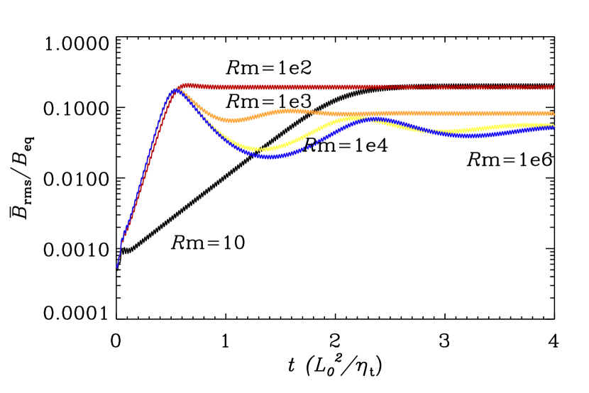
Figure 6: The same that Fig. 4 but for simulations including a diffusive flux of $\alpha_{\rm M}$. All the simulations correspond to $\kappa_{\alpha}=0.005\eta_{\rm t}$.

Besides its dependence on $R_{\rm m}$, the evolution of $\alpha_{\rm M}$ depends also on $\kappa_{\alpha}$. For models with $\kappa_{\alpha}\ll\eta_{\rm t}$, the evolution of $\alpha_{\rm M}$ relies on $R_{\rm m}$, but for $\kappa_{\alpha}\geq 0.1\eta_{\rm t}$, the dissipation time of $\alpha_{\rm M}$ becomes comparable to, or even shorter, than the period of the dynamo cycle. This results in $\alpha_{\rm M}$ becoming oscillatory, as shown in the bottom panel of Fig. 8. The amplitude and the period of these oscillations depend on the value of $\kappa_{\alpha}$.

Figure 7: $R_{\rm m}$ dependence of the averaged mean magnetic field (top), the temporal mean value of ${\alpha_{\rm M}}$ at $r=0.8L_{0}$, $\theta=45^{\circ}$ (middle) and the dynamo cycle period, $T$ in diffusion time units (bottom). The continuous line present the result for simulations without $\alpha_{\rm M}$ diffusive flux ($\kappa_{\alpha}=0$) and the dashed line shows the results for $\kappa_{\alpha}=0.005\eta_{\rm t}$. The error lines in the middle panel indicate the maximum and minimum amplitudes in the oscillations of $\alpha_{\rm M}$ at that point.

Figure 8: Top, final amplitude of the rms mean magnetic field for different values of $\kappa$, in this case $R_{m}=10^{7}$. Bottom, final amplitude of $\alpha_{\rm M}$ at $r=0.8L_{0}$ and $\theta=45^{\circ}$. The error lines indicate the maximum and minimum amplitude in the oscillations of $\alpha_{\rm M}$ at this point.

In the top panel of Fig. 8 we show the final value of the averaged mean magnetic field as a function of $\kappa_{\alpha}$. We observe that for $\kappa_{\alpha}$ in the range $(0.1$–$1)\,\eta_{\rm t}$, the value of $\overline{B}_{\rm rms}$ remains between 20% and 60% of the equipartition, a value similar to the one obtained in the simulations using algebraic $\alpha$ quenching (Section 4.1, Fig. 3). For $\kappa_{\alpha}>\eta_{\rm t}$, super-equipartition values of the magnetic field may be reached. This is because larger values of $\kappa_{\alpha}$ result in oscillations of $\alpha_{\rm M}$ with larger amplitude, such $\alpha_{\rm M}$ may locally change its sign, increasing the value of the total $\alpha$ in each hemisphere and thereby enhancing the dynamo action. Such high values of the diffusion of the magnetic helicity are unlikely in nature.

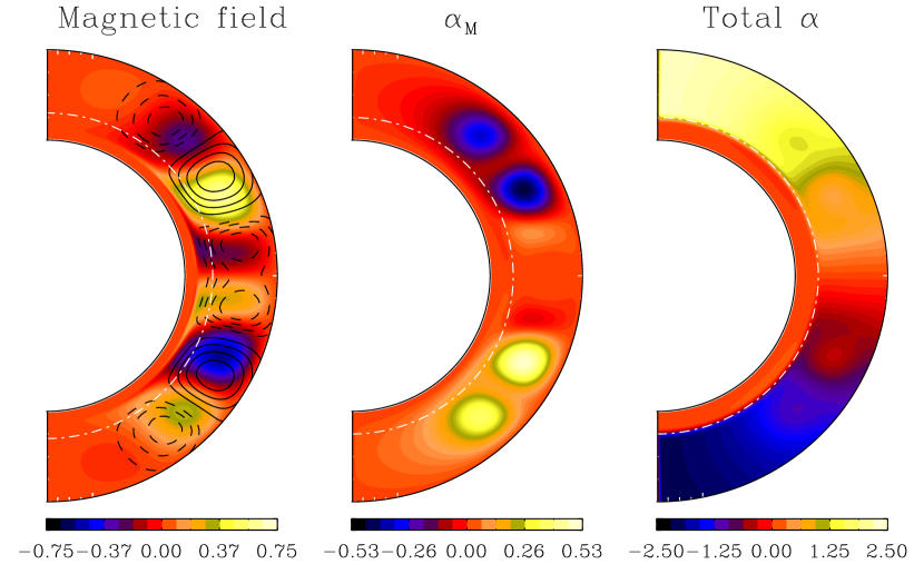
Figure 9: The same than Fig. 5 but for a diffusive flux, with $\kappa=\eta$. The snapshot corresponds to $t=3.0$ ($L_{0}/\eta_{\rm t}$).

4.4 The Vishniac-Cho flux

Our next step is to explore the magnetic helicity flux proposed by Vishniac & Cho (2001) in the form given by equation (8). For the moment we set $\kappa_{\alpha}=0$. In a previous study on the effects of the VC flux in a MFD model in Cartesian coordinates, Brandenburg & Subramanian (2005b) found that there exist a critical value for the parameter $C_{\rm VC}$ above which there is a runaway growth of the magnetic field that can only be stopped using an additional algebraic quenching similar to the one used in Section 4.1. They found that this critical value, $C_{\rm VC}*$, diminishes with increasing the amount of shear. Since we have used a strong shear ($C_{\Omega}=-10^{4}$) we use nominal values of $C_{\rm VC}=10^{-3}$, but without any algebraic quenching.

The term $\bm{\nabla}\cdot\overline{\bm{{\cal F}}}_{\rm VC}$ develops a multi-lobed pattern which travels in the same direction as the dynamo wave, this confirms that the VC flux follows the lines of iso-rotation. From equation (8), we see that the VC flux is proportional to the magnetic energy density. In the present case, with $C_{\Omega}\gg C_{\alpha}$, the spatial distribution of $\bm{\nabla}\cdot\bm{\overline{\cal F}}_{\rm VC}/B^{2}_{\rm eq}$ is dominated by the terms involving $B_{\phi}^{2}$ in equations. 9-11 (this may be inferred from the left hand panels of Fig. 10a). This results in a new distribution of $\alpha_{\rm M}$, with concentrated regions of positive (negative) sign at low latitudes in the northern (southern) hemisphere, and a broad region of negative (positive) sign in latitudes between $20^{\circ}$ and $60^{\circ}$ latitude (see middle panels of Fig. 10). Surprisingly we find that the general effect of this flux is to decrease the final amplitude of the magnetic field with respect to the case without any fluxes as can be seen in Fig. 11. Note that we have until now used only the potential field boundary condition for the poloidal field. When we consider both diffusive as well as VC fluxes, with $\kappa_{\alpha}=0.1\eta_{\rm t}$ and $C_{\rm VC}=10^{-3}$, we obtain a magnetic field of slightly larger amplitude compared to the case with only the diffusive flux (compare the value of $\overline{B}_{\rm rms}$ in Runs DRm1e3 and VCD in Table 1). However we may say from the butterfly diagram of Fig. 12 that the toroidal magnetic field appears to be more concentrated at lower latitudes, where the sign of $\alpha_{\rm M}$ is same as that of $\alpha_{\rm K}$.

With negative values of $C_{\rm VC}$, it was found that the resulting profile of $\alpha_{\rm M}$ is only weakly modified from cases without fluxes, though its value is reduced marginally such that the final amplitude of $\overline{B}_{\rm rms}$ is slightly larger. But even this contribution does not help in alleviating catastrophic quenching in models with large $R_{\rm m}$ (see Fig. 11).

Since VC fluxes transport helicity along lines of constant shear, it may be expected that they are more important in models with latitudinal shear, since in this case the magnetic helicity flux can travel either towards the bottom or the top boundaries, from where magnetic helicity can be expelled. For testing this possibility, we turn off the radial shear profile and consider a purely latitudinal solar-like differential rotation:

$$\Omega(r,\theta)=C_{\Omega}\left(\frac{\eta_{\rm t}}{\Omega_{\rm eq}L_{0}^{2}}\right)\Theta(r,r_{2},w_{1})(\Omega_{s}(\theta)-\Omega_{c})\;,$$ (17)

where $\Omega_{\rm eq}/2\pi=460.7$ nHz is the angular velocity at the equator, and $\Omega_{s}(\theta)=\Omega_{\rm eq}+a_{2}\cos^{2}\theta+a_{4}\cos^{4}\theta$ gives the latitudinal profile, with $a_{2}/2\pi=-62.9$ nHz and $a_{4}/2\pi=-67.13$ nHz.

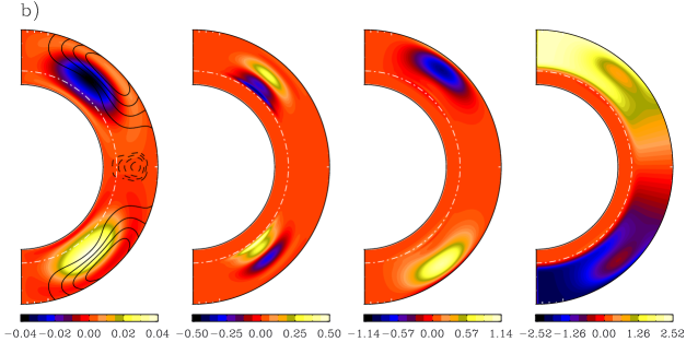
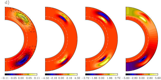
Figure 10: Meridional snapshots of different models the in Table 1: a) model VCa, b) model VC_θa, c) model VCD_θ and d) model VC_θvf. The contours (colors and lines) for the magnetic field have the same meaning than in Fig. 5. In this plot we have include a new column with the value of the VC component in the $\alpha_{\rm M}$ equation, i.e., $\bm{\nabla}\cdot\bm{\overline{\cal F}}_{\rm VC}/B^{2}_{\rm eq}$. All the snapshots corresponds to the relaxed state of evolution.

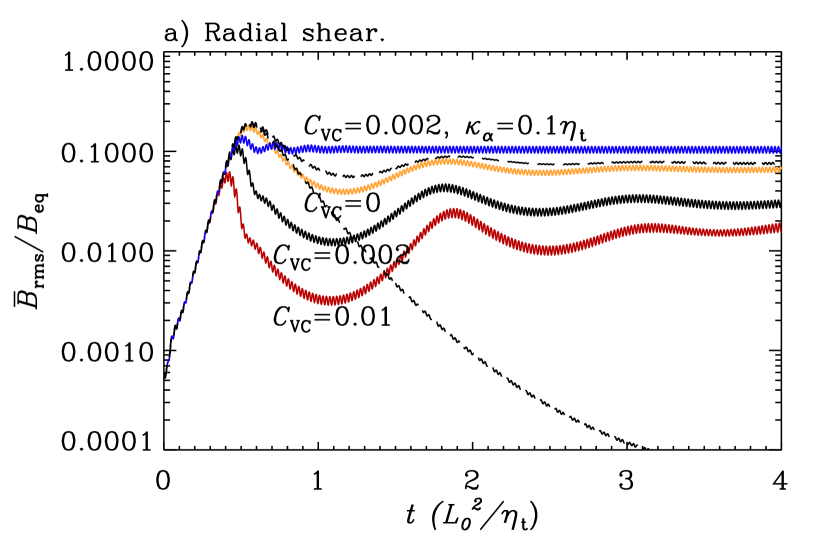
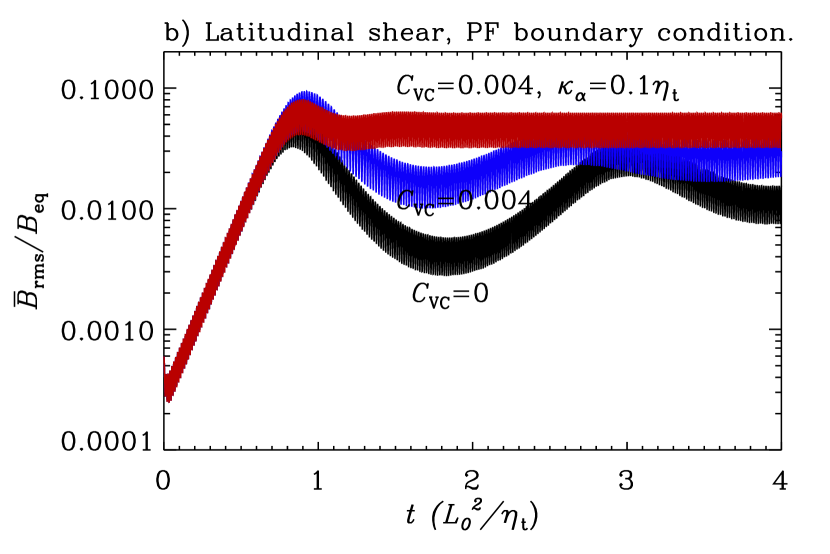
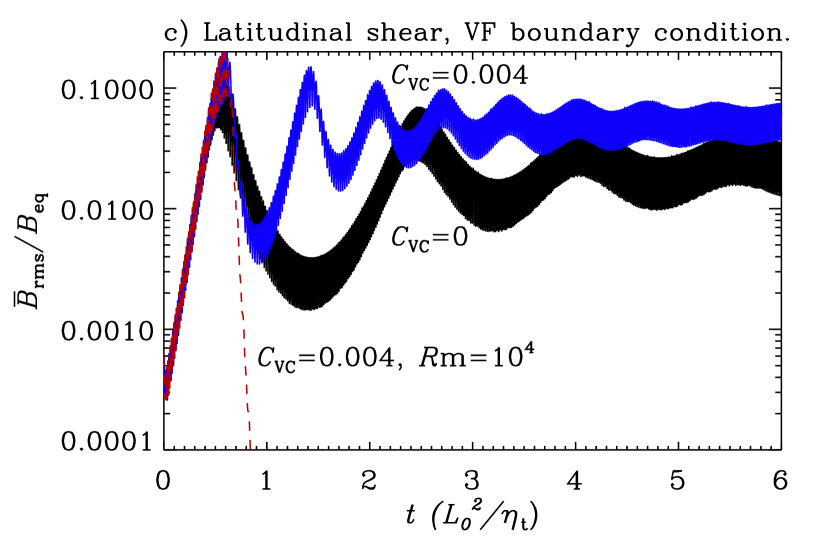
Figure 11: Time evolution of the averaged mean magnetic field for different values of $C_{\rm VC}$: a) Radial shear, b) latitudinal shear with potential field boundary conditions and c) latitudinal shear with vertical field boundary conditions. The width of the different bands reflects the range over which the magnetic field varies during one cycle. Note that the cycle period is short compared with the resistive time scale on which the magnetic field reaches its final saturation. If not indicated, in all models $R_{\rm m}=10^{3}$. The two dashed lines in the panel a) corresponds to $C_{vc}=-0.002$ for $R_{\rm m}=10^{3}$ and $R_{\rm m}=10^{4}$.

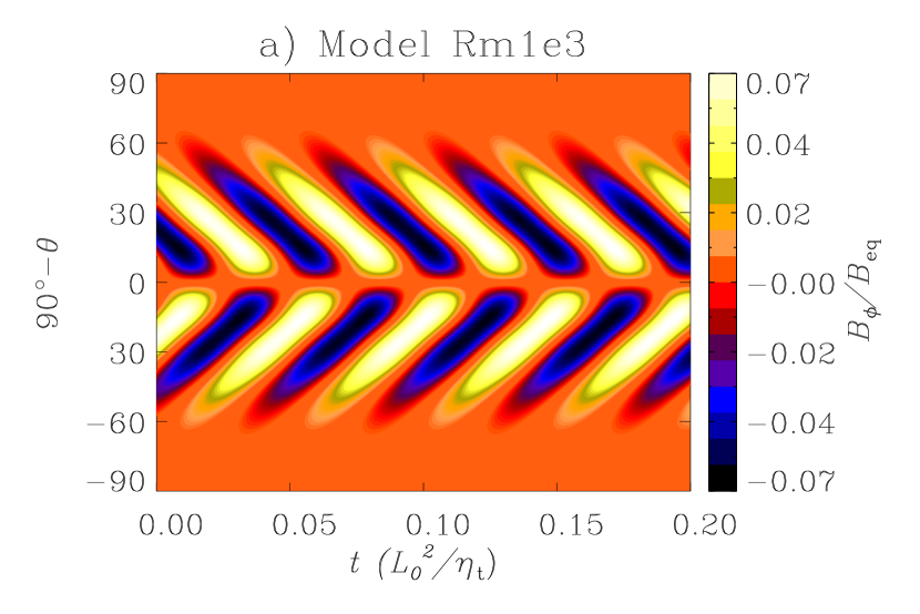
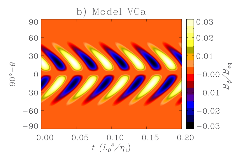
Figure 12: Butterfly diagrams of toroidal field for runs without magnetic helicity flux (a) and with VC flux (b) for $R_{\rm m}=10^{3}$. Note the stronger concentration of magnetic field at lower latitudes in the presence of VC flux.

In order for the dynamo to be slightly supercritical, as in the previous cases, we consider $C_{\Omega}=5\times 10^{4}$. This dynamo solution corresponds to a dynamo wave produced at mid latitudes ($\sim 45^{\circ}$) that travels upwards (since $C_{\Omega}$ now is positive). As in the previous cases with radial shear, the distribution of $\bm{\nabla}\cdot\bm{\overline{\cal F}}_{\rm VC}/B^{2}_{\rm eq}$ is similar to that of the divergence of magnetic energy density (left hand panels of Fig. 10 b,c and d). If no fluxes are considered, the final amplitude of the mean magnetic field is $\sim 0.03$% of the equipartition value. In presence of VC fluxes, starting with $C_{\rm VC}=10^{-3}$ for a model with $R_{\rm m}=10^{3}$, we notice that the final magnetic field is twice as large as in the case with $C_{\rm VC}=0$.

Our model becomes numerically unstable beyond $C_{\rm VC}=10^{-2}$ due to appearance of concentrated regions of strong $\alpha_{\rm M}$. When VC and diffusive fluxes are considered simultaneously, with $C_{\rm VC}=10^{-3}$ and $\kappa_{\alpha}=0.1\eta_{\rm t}$, the relaxed value of $\overline{B}_{\rm rms}$ is only slightly below the value reached at the end of the kinematic phase (Fig. 11b). In this case $\alpha_{\rm M}$ spreads out in the convection zone, as shown in Fig. 10c, indicating that the effects of the VC flux are not important when compared with the diffusive flux.

We repeated the calculation by considering the vertical field (VF) boundary condition, $\partial(rB_{\theta})/\partial\theta=0$, for the top boundary, instead of the potential field (PF) condition used throughout the rest of this work. Furthermore, in the models with VF conditions the presence of the VC flux leads to an increase of $B_{\rm sat}$ by a factor of $\sim 2$ compared to the case without VC flux (see Fig. 11c). It may be noted that $\alpha_{\rm M}$ shows regions of both positive and negative signs in each hemisphere (see Fig. 10d). Thus, the total $\alpha$ effect is increased locally to values well above the kinematic one. This implies that in the region around $\pm 45^{\circ}$ the dynamo action is driven by the magnetic $\alpha$ effect. A similar secondary dynamo is found to be working for a different distribution of shear and $\alpha_{\rm K}$ (Chatterjee, Guerrero & Brandenburg, 2010). As with PF boundary condition, large values of $C_{\rm VC}$ result in a numerical instability of the magnetic field in the simulation with VF.

The main result of this section is that the VC flux does not alleviate catastrophic quenching of the dynamo for large values of $R_{\rm m}$ (see the dashed lines in Fig. 11 a and c). The reason for this may be related to the fact that the radial flux has components that are either proportional to $B_{\theta}$ or to $B_{\phi}$ (equation 9). As $B_{\phi}$ vanishes on the top boundary, and $B_{\theta}$ is small, the VC flux is not able to dispose of $\alpha_{\rm M}$ across the boundary. This might change if diffusive fluxes became important near the top or if a different boundary condition on $B$ were applied.

5 Conclusions

We have developed $\alpha\Omega$ dynamo models in spherical geometry with relatively simple profiles of $\alpha_{\rm K}$ and shear ($\partial\Omega/\partial r$ and $\partial\Omega/\partial\theta$). We choose potential field (also vertical field in some cases) and perfect conductor boundary conditions for the top and bottom boundaries, respectively. We estimate the critical dynamo number by fixing $C_{\Omega}=-10^{4}$ and varying $C_{\alpha}$ while using algebraic quenching.

Using a dynamo number, $C_{\Omega}C_{\alpha}$, that is slightly super-critical, we solve the induction equations for $B$ and $A$ together with an equation for the dynamical evolution of the magnetic $\alpha$ effect or $\alpha_{\rm M}$. We find that for positive (negative) values of $C_{\alpha}$ in the northern (southern) hemisphere, $\alpha_{\rm M}$ is mainly negative (positive), with narrow fractions of opposite sign in regions where $\alpha_{\rm K}$ or $\overline{B}$ are equal to zero.

We find that the kinematic phase is independent of $R_{\rm m}$. However for $R_{\rm m}>10^{2}$ there exists a phase of relaxation post saturation in which the averaged magnetic field oscillates about a certain mean. The larger the $R_{\rm m}$, the more pronounced are the damped oscillations and the longer is the relaxation time (Fig. 4). The final value of the magnetic energy obeys a $R_{\rm m}^{-1}$ dependency ($R_{\rm m}^{-0.5}$ for magnetic field, Fig. 7), which is in agreement with earlier work (Brandenburg & Subramanian, 2005b; Brandenburg, Candelaresi & Chatterjee, 2009).

We argue that including equation (6) in MFD models is appropriate for describing the quenching of the magnetic field in the dynamo process. Since we observe large-scale magnetic fields at high magnetic Reynolds numbers in astrophysical objects, there must exist a mechanism to prevent the magnetic field from catastrophic quenching.

We have studied the role that diffusive and VC fluxes may play in this sense. Their contribution may be summarized as follows:

1. In the presence of diffusive fluxes, $\alpha_{\rm M}$ has only one sign in each hemisphere (negative in the northern hemisphere and positive in southern) and is evenly distributed across the dynamo region (Fig. 9).

2. For $R_{\rm m}<10^{2}$ the mean values of $\alpha_{\rm M}$ are similar to models without diffusive fluxes, whereas for $R_{\rm m}\geq 10^{2}$, $\alpha_{\rm M}$ has smaller values that seem to be independent of $R_{\rm m}$ (see Fig. 7, middle).

3. Even a very low diffusion coefficient, e.g. $\kappa_{\alpha}=0.001\eta_{\rm t}$, causes $\overline{B}_{\rm rms}$ to depart from the $R_{\rm m}^{-0.5}$ tendency and converge to a constant value which is then around $5$% of the equipartition value for large values of $R_{\rm m}$, but below the value of $10^{7}$ used in this study (dashed line in Fig. 7, top).

4. Larger values of $\kappa_{\alpha}$ result in larger final field strengths.

5. In models with only radial shear the Vishniac-Cho flux contributes to $\alpha_{\rm M}$ with a component that travels in the same direction as the dynamo wave. This produces a different radial and latitudinal distribution of the magnetic $\alpha$ effect that also affects the distribution of the magnetic fields. However, it does not help in alleviating the quenching at high $R_{\rm m}$. On the contrary, the larger the coefficient $C_{\rm VC}$, the smaller is the resultant magnetic field.

6. In models with only latitudinal shear the VC flux travels radially outward but it remains concentrated at the center of the dynamo region. In a given hemisphere the resultant distribution of $\alpha_{\rm M}$ has both positive and negative signs. The part of $\alpha_{\rm M}$ that has the same sign as $\alpha_{\rm K}$ enhances dynamo action. This effect is more evident in models with vertical field boundary conditions (Figs. 10b-d).

7. In models with vacuum and vertical field boundary conditions and $R_{\rm m}=10^{3}$, the VC flux increases the final value of the magnetic field by a factor of two compared to the case without any fluxes.

8. The magnetic field in models with $R_{\rm m}\geq 10^{4}$ and with non-zero VC flux decays after the kinematic phase since the total $\alpha$ effect becomes subcritical (see dashed lines in Fig. 11 a and c).

9. Larger values of $C_{\rm VC}$ produce narrow bands of $\alpha_{\rm M}$ which drives intense dynamo action in these regions. This positive feedback between the magnetic field and $\alpha_{\rm M}$ causes the simulation to become numerically unstable in the absence of any other quenching effect.

From the above results it is clear that diffusive fluxes are much more important in alleviating catastrophic quenching when compared to the Vishniac & Cho fluxes (in the form of equation 8) for a large range of $R_{\rm m}$. This is somehow intriguing since it is known from DNS that shear in domains with open boundaries does indeed help in alleviating the catastrophic quenching. It may be understood as a result of the large value of $C_{\Omega}$ compared with $C_{\alpha}$ and also to the top boundary condition for the azimuthal magnetic field (Brandenburg, 2005; , 2008).

The results presented above indicate that considerable work is still necessary in order to understand the role of larger-scale shear in transporting and shedding small-scale magnetic helicity from the domain.

In snapshots of the meridional plane as well as in butterfly diagrams we notice that the diffusive fluxes do not significantly modify the morphology and the distribution of the magnetic field when compared with cases without fluxes or even with simulations with algebraic $\alpha$ quenching. On the other hand, for models with VC flux the distribution of $\alpha_{\rm M}$ becomes different and so does the magnetic field. This is clear from the butterfly diagram shown in Fig. 12b, which exhibits a magnetic field confined to equatorial latitudes reminiscent of the observed butterfly diagram of the solar cycle. Even though this result corresponds to a simplified model, it illustrates the importance of considering the dynamical $\alpha$ quenching mechanism for modeling the solar dynamo. Similar changes in the distribution of $\alpha_{\rm M}$ and $\bm{\overline{B}}$ are expected to happen when advection terms are included in the governing equations.

In the simulations presented here, $\Omega$ and $\alpha$ effects are present in the same layers. An interesting question is whether the quenching of the dynamo is catastrophic when both layers are segregated, as in the Parker’s interface dynamo or the flux-transport dynamo models. We address this question in detail in two companion papers (Chatterjee, Brandenburg & Guerrero, 2010; Chatterjee, Guerrero & Brandenburg, 2010).

We should notice that the back reaction of the magnetic field affects not only the $\alpha$ effect, but also the other dynamo coefficients, including the turbulent diffusivity. Contrary to quenching of $\alpha$, the quenching of $\eta_{\rm t}$ may be considered through an algebraic quenching function (see e.g. Yousef, Brandenburg & Rüdiger, 2003; Käpylä & Brandenburg, 2009). (2009) have shown that in a flux-transport model these effects could affect properties of the models such as the final magnetic field strength and its distribution in radius and latitude. We leave the study of models with simultaneous dynamical $\alpha$ and $\eta$ quenchings for a future paper. Solar-like profiles of differential rotation and meridional circulation along with dynamical $\alpha$ quenching will also be considered in a forthcoming paper.

References

- Berger & Ruzmaikin (2000) Berger, M. A. and Ruzmaikin, A., 2000, JGR, 105, 10481
- Blackman & Brandenburg (2002) Blackman, E. G. and Brandenburg, A., 2002, ApJ, 579, 359
- Brandenburg (2005) Brandenburg, A. 2005, ApJ, 625, 539
- Brandenburg & Subramanian (2005a) Brandenburg, A. and Subramanian, K., 2005a, Phys. Rep., 417, 1
- Brandenburg & Subramanian (2005b) Brandenburg, A. and Subramanian, K., 2005b, Astron. Nachr., 326, 400
- Brandenburg et al. (2007) Brandenburg, A., Käpylä, P. J., Mitra, D., Moss, D. and Tavakol, R., 2007, Astron. Nachr., 328, 1118
- Brandenburg, Candelaresi & Chatterjee (2009) Brandenburg, A., Candelaresi, S. and Chatterjee, P., 2009, MNRAS, 398, 1414
- Brown et al. (2010) Brown, B. P., Browning, M. K., Brun, A. S., Miesch, M. S. and Toomre, J., 2010, ApJ, 711, 424
- Charbonneau & MacGregor (1997) Charbonneau, P. and MacGregor, K. B., 1997, ApJ, 486, 502
- Chatterjee, Nandy & Choudhuri (2004) Chatterjee, P., Nandy, D. and Choudhuri, A. R., 2004, A&A, 427, 1019
- Chatterjee, Brandenburg & Guerrero (2010) Chatterjee, P., Brandenburg, A. and Guerrero, G., 2010, Geophys. Astrophys. Fluid Dyn. (submitted), preprint: NORDITA-2010-34
- Chatterjee, Guerrero & Brandenburg (2010) Chatterjee, P., Guerrero, G. and Brandenburg, A., 2010, A&A (submitted), preprint: NORDITA-2010-35
- Dikpati & Charbonneau (1999) Dikpati, M. and Charbonneau, P., 1999, ApJ, 256, 523
- Dikpati & Choudhuri (1994) Dikpati, M. and Choudhuri, A. R., 1994, A&A, 291, 975
- (15) Guerrero G., de Gouveia Dal Pino, E. M. 2007, A&A, 464, 341
- (16) Guerrero G., de Gouveia Dal Pino, E. M. 2008, A&A, 485, 267
- (17) Guerrero G., de Gouveia Dal Pino, E. M. 2009, ApJ, 701, 725
- (18) Hubbard A., Brandenburg, A., 2010, Geophys. Astrophys. Fluid Dyn., submitted, arXiv:1004.4591
- (19) Käpylä, P. J., Korpi, M. J. and Brandenburg, A., 2008, A&A, 491, 353
- Käpylä & Brandenburg (2009) Käpylä, P. J. and Brandenburg, A., 2009, ApJ, 699, 1059
- Käpylä et al. (2010) Käpylä, P. J., Korpi, M. J., Brandenburg, A., Mitra, D. and Tavakol, R., 2010, Astron. Nachr., 331, 73
- Kleeorin & Rogachevskii (1999) Kleeorin, N. and Rogachevskii, I., 1999, Phys Rev E, 59, 6724
- MacGregor & Charbonneau (1997) MacGregor, K. B. and Charbonneau, P., 1997, ApJ, 486, 484
- Mitra et al. (2010a) Mitra, D., Candelaresi, S., Chatterjee, P., Tavakol, R. and Brandenburg, A., 2010, Astron. Nachr., 331, 130
- Mitra et al. (2010b) Mitra, D., Tavakol, R., Käpylä, P., and Brandenburg, A., 2010, arXiv:0901.2364v2
- Peaceman & Rachford (1955) Peaceman, D. W., Rachford, H. H., 1955 J. Soc. Ind. App. Math., 3, 28
- Pouquet, Frisch & Léorat (1976) Pouquet A., Frisch U., Léorat J. 1976, J. Fluid Mech., 77, 321
- (28) Stix, M., 1972, A&A, 20, 9
- Shukurov et al. (2006) Shukurov, A., Sokoloff, D. Subramanian, K. and Brandenburg, A., 2006, A&A, 448, L33
- Subramanian & Brandenburg (2004) Subramanian, K. and Brandenburg, A., 2004, Phys Rev Lett, 93, 205001
- Vishniac & Cho (2001) Vishniac, E.T. and Cho, J., 2001, ApJ, 550, 752,
- Zhang et al. (2006) Zhang, H., Sokoloff, D., Rogachevskii, I., et al., 2006, MNRAS, 365, 276
- Yousef, Brandenburg & Rüdiger (2003) Yousef, T. A., Brandenburg, A. and Rüdiger, G., 2003, A&A, 411, 321