Inference of Gene Predictor Set Using Boolean Satisfiability

Abstract

The inference of gene predictors in the gene regulatory network has become an important research area in the genomics and medical disciplines. Accurate predicators are necessary for constructing the GRN model and to enable targeted biological experiments that attempt to confirm or control the regulation process. In this paper, we implement a SAT-based algorithm to determine the gene predictor set from steady state gene expression data (attractor states). Using the attractor states as input, the states are ordered into attractor cycles. For each attractor cycle ordering, all possible predictors are enumerated and a CNF expression is formulated which encodes these predictors and their biological constraints. Each CNF is explored using a SAT solver to find candidate predictor sets. Statistical analysis of the results selects the most likely predictor set of the GRN corresponding to the attractor data. We demonstrate our algorithm on attractor state data from a melanoma study [1] and present our predictor set results.

I Introduction

With the mapping of the human genome complete, the focus in computational biology has shifted from sequence analysis to the understanding of gene regulation and its inter-relation with the biological system. The use of genome information has given rise to the notion of ”personalized medicine” – targeted and specific disease prevention and treatment based on individual gene information [2, 3]. The urgent applications to cancer and gene-related diseases calls for the genomics field to significantly improve the algorithms used for accurate inference of the gene regulatory network (GRN).

In an organism, the genome is a highly complex control system wherein proteins and RNA produced by genes interact with and regulate the activity of other genes [4]. The activity of a target gene $g_{i}$ is regulated (or predicted) by the genes in its predictor (e.g. if $g_{1}$ becomes inactive when $g_{2}$ and $g_{3}$ are active, then $g_{2}$ and $g_{3}$ are called predictors of g). The complete set of predictors (predictor set), which contains the predictors for each gene in the GRN, describes the interaction of all genes within the gene regulatory network and is the prerequisite for inferring the GRN structure.

There are several GRN characteristics that impact the formulation of our GRN model and predictor inference algorithm. First, the gene activity level of all genes at a particular time $t$ represents the state of the GRN at that time $t$. From our knowledge of biological systems, we observe that over time, cellular processes transition to stable attractor states. Some of these attractor states represent normal cellular phenomena in biology such as cell cycle and division. However, some attractor states are consistent with disease such as the metastasis of cancer. Second, the GRN is often inferred by observing microarray-based experimental data which measures the activity level of genes. The correlation of the observed gene activity (or state) can be used to help describe the gene regulation. The disadvantage of using microarray data is such that studies do not involve controlled time experimental data (time-series data). Hence the measurements are assumed to arise from the cyclic sequence of gene expressions (attractor states) in steady state (attractor cycles). The GRN is then inferred from this data, using methods traditionally based on probabilistic transition models [5, 6].

As previously mentioned, it is necessary to determine the predictor set to reconstruct the GRN. However, there may exist many possible predictors for any gene, based on the attractor cycle data. Furthermore, only certain combinations of predictors may form a valid predictor set due to biological constraints. The issue addressed in this paper is how to efficiently and deterministically select the predictors that form the predictor set. We have implemented a Boolean satisfiability (SAT) based algorithm for the inference of gene predictors. Satisfiability is a decision problem of determining whether the variables in a Boolean formula (expressed in Conjunctive Normal Form or CNF) can be assigned to make the formula evaluate to true. Although SAT is NP-complete, many SAT solvers have been developed to quickly and efficiently solve large SAT problems. Our algorithm takes advantage of advanced SAT solvers to find the predictor set.

The basic outline of our SAT-based algorithm is described briefly below. First, all possible orderings of attractor state are enumerated, yielding all possible attractor cycles. For each ordering, we enumerate all predictors that are logically valid, and create a CNF expression which encodes all these predictors and biological constraints (such as cardinality bounds on the predictors). A SAT solver is used to find the valid candidate predictor sets. After this process is done iteratively for all attractor cycle (orderings), statistical analysis provides the most likely candidates for the predictor set.

The key contributions of this paper are:

• We develop a Boolean Satisfiability based approach to realize the gene predictor set from attractor state data.

• We modify an existing SAT-solver (MiniSat [7]) for efficient all-SAT computation and further optimize MiniSat for improved predictor inference.

• On gene expression data from a melanoma study [1], we apply our SAT-based algorithm and present results for genes that regulate all the genes, including the cancer gene WNT5a.

• Our approach can be used to find the predictor set for any gene related disease, provided attractor state data is available. The predictor set information obtained from our algorithm can be used by biologists to fine tune their gene expression experiments.

The remainder of this paper is organized as follows. Section II describes previous work in modeling the gene regulatory network and inference of gene predictors. Section III presents our FSM model and Boolean SAT approach. Section IV reports experimental results. Concluding comments and future work are discussed in Section V.

II Previous Work

Several models have been proposed for modeling the GRN such as Markov Chains [8, 9], Coupled ODEs (ordinary differential equations), Boolean Networks [10, 11], Continuous Networks [12], and Stochastic Gene Networks [13].

This paper utilizes the Boolean Network (BN) model that was proposed by Kauffman in 1969 [10]. In a Boolean Network, the expression activity of a gene is represented as a binary value, where 1 indicates the gene is ON (active) and producing gene-products, while 0 indicates it is OFF. Such a model cannot capture the continuous and stochastic biochemical properties of protein and RNA production. However, genes can typically be modeled as ON or OFF in any particular biochemical pathway.

In [14, 15], the probabilistic modeling framework is represented by dynamic Bayesian networks and probabilistic Boolean networks (PBNs). The method proposed considers gene prediction using multinomial probit regression with Bayesian variable selection. Genes are selected which satisfy multiple regression equations, of which the strongest genes are used to construct the predictor set. The target gene is predicted based on the strongest genes, using the coefficient of determination to measure predictor accuracy.

Another method proposed by [16] also assumes PBN. A partial state transition table is constructed based on available attractor state data. From this state transition table, predictors with 3 or less regulating genes are selected for each target gene. All unknown values in the table are randomly set. The Boolean network is simulated for several iterations on several starting states, observing whether the states eventually transition to an attractor cycle. If the simulation successfully transitions to attractor cycles, the selected predictors are considered as a valid predictor set. This process is repeated to build a collection of Boolean Networks which are combined to form a Probabilistic Boolean Network (PBN).

Our larger goal is to find a small number of deterministic GRNs, rather than a PBN. Towards this, we need to find ways to accurately find the predictor set. This is the focus of this paper. Philosophically, our aim is to invest effort into accurate predictor set determination, so that the results can be used to find high quality deterministic GRNs.

III Our Approach

This section describes our model and algorithm for inference of predictor sets using SAT. We begin with some logic synthesis definitions which are useful in understanding the application of SAT to GRNs and predictor selection. We then describe a simple example to explain the algorithm. Lastly, we generalize the algorithm for larger problem sets and comment on specific issues about the use of SAT and complexity.

III-A Definitions

Definition 1

A literal or a literal function is a binary variable $x$ or its negation $\overline{x}$.

Definition 2

A cube is a product of a set of literal functions.

Definition 3

A clause is a disjunction containing literals.

Definition 4

A Conjunctive Normal Form (CNF) expression consists of a conjuction (AND) of $m$ clauses $c_{1}\ldots c_{m}$. Each clause $c_{i}$ consists of disjunction (OR) of $k$ number of literals.

A CNF formula is also referred to as a logical product of sums. Thus, to satisfy the formula, each clause must have at least one literal evaluate to true.

Definition 5

Boolean satisfiability (SAT). Given a Boolean formula $S$ on a set of binary variables $X$ , expressed in Conjunctive Normal Form (CNF), the objective of SAT is to identify an assignment of the binary variables in X that satisfies $S$, if such an assignment exists.

For example, consider the formula $S(a,b,c)=(a+\overline{b})\cdot(a+b+c)$. This formula consists of 3 variables, 2 clauses, and 4 literals. This particular formula is satisfiable, and a satisfying assignment is $<a,b,c>\,=\,<0,0,1>$, which can be expressed as the satisfying cube $\overline{a}\overline{b}c$.

There may exist many satisfying assignments for the formula in question. An extension of the SAT problem is to find all satisfying assignments (or All-SAT). One simple method to accomplish All-SAT is to repeatedly run SAT on the formula $S$, express each satisfying assignment as a cube $k$, complement $k$ to get a clause $c$, and add $c$ as a new clause of the formula and running SAT again. The inclusion of $c$ in $S$ ensures that the same cube $k$ cannot be found as a satisfying assignment again. The process continues until no new solutions can be found. In the previous example, the satisfying cube $\overline{a}\overline{b}c$ is complemented and added as a new clause $(a+b+\overline{c})$ to the original formula to be solved by SAT again (this is repeated until no new satisfying assignments are found).

Definition 6

A predictor $f_{i}=\{g_{j},g_{k},\cdots\}$ lists the set $\{g_{j},g_{k},\cdots\}$ of genes which regulate the activity of gene $g_{i}$.

Definition 7

The predictor set is the complete set of predictors {$f_{1},f_{2},\cdots,f_{n}$} for the GRN with $n$ genes $g_{1},g_{2},\cdots,g_{n}$.

III-B Implementation and Example

Given gene expression data (a set of attractor states) as input, we would like to determine the best predictor set. We first present an outline of our SAT-based algorithm, and then explain the steps through a simple example.

The algorithm has three main steps.

• First, attractor states are ordered into attractor cycles. For each possible ordering of the attractor states in to attractor cycles, all possible predictors are found and a CNF is generated containing the predictors and constraints.

• Second, the CNF is solved for All-SAT, recording all satisfying cubes. Each cube corresponds to a predictor set. The first two steps are repeated for all attractor cycle orderings.

• Finally, statistical analysis on the SAT results determines the most frequent (likely) predictor set for the GRN.

We apply the SAT-based algorithm to a simple example with three genes $(g_{1},g_{2},g_{3})$ and gene expression data with two lines $(000,101)$. The present state of these genes is represented by the variables $<x_{1},x_{2},x_{3}>$ and the next state is represented by the variables $<y_{1},y_{2},y_{3}>$. We assume each line was measured in steady state and therefore is an attractor state.

Step 1: We order (or arrange) the attractor states into valid attractor cycles, of which there are two possibilities. One ordering is with each attractor state transitioning to itself with a self-edge, thus resulting in an attractor cycle of length one, as shown in Table I. The other possible ordering is a transition from one state to the other and back, forming a single attractor cycle of length two.

For each valid attractor cycle ordering, a partial state transition table is constructed containing the attractor states. For example, if the first attractor cycle ordering (in which states transition to themselves) is chosen, the resulting state transition table is shown in Table I. To find all valid predictors of a gene, each next state column is checked against all combinations of the present state columns. For example with gene $g_{1}$, the next state bit $y_{1}$ is $0$ in the first row and $1$ in the second row. Hence the present state bit $x_{2}$ alone cannot predict $y_{1}$ as there is a contradiction (since $y_{1}=0$ from the first row and $y_{1}=1$ in the second row and $x_{2}=0$ for both rows). However if we consider state bits $x_{2}$ and $x_{3}$, we find that they together can predict $y_{1}$, since the pair of values $<x_{2},x_{3}>$ is different in the two rows. Thus gene $g_{1}$ can be regulated by genes $g_{2}$ and $g_{3}$, so one valid predictor for $g_{1}$ is $f_{1}=\{x_{2},x_{3}\}$. All valid predictors with 3 or less inputs are exhaustively searched and recorded for CNF formulation in the next step. In our example, gene $g_{1}$ has 5 possible predictors $\{x_{3}\},\ \{x_{1},x_{2}\},\ \{x_{1},x_{3}\},\ \{x_{2},x_{3}\},\ \{x_{1},x_{2},x_{3}\}$ which we label $v^{1}_{1},v^{1}_{2},v^{1}_{3},v^{1}_{4}$ respectively. We assume that a gene cannot self-regulate, so $\{x_{1}\}$ is not a valid predictor.

Present state			Next state
$x_{1}$	$x_{2}$	$x_{3}$	$f_{1}$	$f_{2}$	$f_{3}$
0	0	0	0	0	0
1	0	1	1	0	1

TABLE I: Example state transition table

Step 2: After all predictors are found, we generate the SAT formula which encodes valid predictor sets for all possible predictor combinations. Each predictor is assigned a variable $v^{i}_{j}$ which corresponds to the $j^{th}$ predictor for gene $i$. Gene $g_{1}$ in our example will have five predictor variables $v^{1}_{1}\equiv\{x_{3}\},\,v^{1}_{2}\equiv\{x_{1},x_{2}\},\,v^{1}_{3}\equiv\{x_{1},x_{3}\},\,v^{1}_{4}\equiv\{x_{2},x_{3}\},\,v^{1}_{5}\equiv\{x_{1},x_{2},x_{3}\}$. Gene $g_{2}$ will have the predictor variables $v^{2}_{1}\equiv\{x_{1},x_{2}\},\,v^{2}_{2}\equiv\{x_{1},x_{3}\},\,v^{2}_{3}\equiv\{x_{2},x_{3}\},\,v^{2}_{4}\equiv\{x_{1},x_{2},x_{3}\}$. Gene $g_{3}$ will have the predictor variables $v^{3}_{1}\equiv\{x_{1}\},\,v^{3}_{2}\equiv\{x_{1},x_{2}\},\,v^{3}_{3}\equiv\{x_{1},x_{3}\},\,v^{3}_{4}\equiv\{x_{2},x_{3}\},\,v^{3}_{5}\equiv\{x_{1},x_{2},x_{3}\}$. There are three constraints that we incorporate while constructing the CNF. The conjuction of these constraints our final CNF.

1. The first constraint $(S_{1})$ is that all genes in the GRN must have a predictor. In other words, we assume that all genes are ”participating” in the GRN and that all genes predict at least one other gene. For gene $i$, all of its associated predictor variables are written in a single clause $c^{1}_{i}=(v^{i}_{1}+\cdots+v^{i}_{j})$. The clause for gene $g_{1}$ in our example is formulated as $c^{1}_{1}=(v^{1}_{1}+v^{1}_{2}+v^{1}_{3}+v^{1}_{4}+v^{1}_{5})$. To satisfy this satisfy this clause, at least one predictor among $v^{1}_{1},\cdots,v^{1}_{5}$ must be chosen. Then to ensure at least one predictor is chosen for all genes we write the conjunction of all $c^{1}_{i}$ clauses.

   $S_{1}=c^{1}_{1}\cdot c^{1}_{2}\cdot c^{1}_{3}$

   $S_{1}=(v^{1}_{1}+v^{1}_{2}+v^{1}_{3}+v^{1}_{4}+v^{1}_{5})\cdot(v^{2}_{1}+v^{2}_{2}+v^{2}_{3}+v^{2}_{4})\cdot(v^{3}_{1}+v^{3}_{2}+v^{3}_{3}+v^{3}_{4}+v^{3}_{5})$

2. The second constraint $(S_{2})$ specifies that for each gene, there exists only one predictor. A gene cannot be regulated by multiple sets of predictors. To formulate the clauses $c^{2}_{i}$ for gene $i$, smaller clauses are formed from all pair combinations of its predictors $v^{i}_{1\cdots j}$. In each of these clauses of pair of variables, both predictor variables are complemented. For gene $g_{1}$, $c^{2}_{1}=(\overline{v^{1}_{1}}+\overline{v^{1}_{2}})\cdot(\overline{v^{1}_{1}}+\overline{v^{1}_{3}})\cdot(\overline{v^{1}_{1}}+\overline{v^{1}_{4}})\cdot(\overline{v^{1}_{1}}+\overline{v^{1}_{5}})\cdot(\overline{v^{1}_{2}}+\overline{v^{1}_{3}})\cdot(\overline{v^{1}_{2}}+\overline{v^{1}_{4}})\cdot(\overline{v^{1}_{2}}+\overline{v^{1}_{5}})\cdot(\overline{v^{1}_{3}}+\overline{v^{1}_{4}})\cdot(\overline{v^{1}_{3}}+\overline{v^{1}_{5}})\cdot(\overline{v^{1}_{4}}+\overline{v^{1}_{5}})$ Any selection of two or more predictors for gene 1 will result in a unsatisfiable solution. Because the $c^{1}_{i}$ clause ensures at least one predictor will be chosen, $c^{2}_{i}$ forces our selection to choose at most one predictor gene $i$. Then constraint $S_{2}$ includes $c^{2}_{i}$ so that at most one predictor is chose for each gene.

   $S_{2}=c^{2}_{1}\cdot c^{2}_{2}\cdot c^{2}_{3}$, where

   $c^{2}_{1}=(\overline{v^{1}_{1}}+\overline{v^{1}_{2}})\cdot(\overline{v^{1}_{1}}+\overline{v^{1}_{3}})\cdot(\overline{v^{1}_{1}}+\overline{v^{1}_{4}})\cdot(\overline{v^{1}_{1}}+\overline{v^{1}_{5}})\cdot(\overline{v^{1}_{2}}+\overline{v^{1}_{3}})\cdot(\overline{v^{1}_{2}}+\overline{v^{1}_{4}})\cdot(\overline{v^{1}_{2}}+\overline{v^{1}_{5}})\cdot(\overline{v^{1}_{3}}+\overline{v^{1}_{4}})\cdot(\overline{v^{1}_{3}}+\overline{v^{1}_{5}})\cdot(\overline{v^{1}_{4}}+\overline{v^{1}_{5}})$

   $c^{2}_{2}=(\overline{v^{2}_{1}}+\overline{v^{2}_{2}})\cdot(\overline{v^{2}_{1}}+\overline{v^{2}_{3}})\cdot(\overline{v^{2}_{1}}+\overline{v^{2}_{4}})\cdot(\overline{v^{2}_{2}}+\overline{v^{2}_{3}})\cdot(\overline{v^{2}_{2}}+\overline{v^{2}_{4}})\cdot(\overline{v^{2}_{3}}+\overline{v^{2}_{4}})$

   $c^{2}_{3}=(\overline{v^{3}_{1}}+\overline{v^{3}_{2}})\cdot(\overline{v^{3}_{1}}+\overline{v^{3}_{3}})\cdot(\overline{v^{3}_{1}}+\overline{v^{3}_{4}})\cdot(\overline{v^{3}_{1}}+\overline{v^{3}_{5}})\cdot(\overline{v^{3}_{2}}+\overline{v^{3}_{3}})\cdot(\overline{v^{3}_{2}}+\overline{v^{3}_{4}})\cdot(\overline{v^{3}_{2}}+\overline{v^{3}_{5}})\cdot(\overline{v^{3}_{3}}+\overline{v^{3}_{4}})\cdot(\overline{v^{3}_{3}}+\overline{v^{3}_{5}})\cdot(\overline{v^{3}_{4}}+\overline{v^{3}_{5}})$

3. The last constraint $(S_{3})$ requires that each genes must be used as a predictor for at least one other gene in the satisfying predictor set. A gene that is not used in any predictor does perform any regulation function and could be removed from the GRN. $S_{3}$ ensures that this does not occur. To ensure that gene $g_{i}$ is used in at least one other predictor, we form clauses $c^{3}_{i}$ which includes all predictors that use gene $g_{i}$ as input. To specify that gene $g_{i}$ must be used, we also include a single variable clause $(x_{i})$ to $c^{3}_{i}$ and add an additional literal $\overline{x_{i}}$ to the other other clauses in $c^{3}_{i}$. The clause $(x_{i})$ requires our solution to include gene $g_{i}$ and the $\overline{x_{1}}$ in the other clauses of $c^{3}_{i}$ forces at least one other predictor variable in $c^{3}_{i}$ be selected to satisfy the formula. For example, the $S_{3}$ clauses for gene $g_{1}$ are $c^{3}_{1}=(x_{1})\cdot(\overline{x_{1}}+v^{1}_{2}+v^{1}_{3}+v^{1}_{5}+v^{2}_{1}+v^{2}_{2}+v^{2}_{5}+v^{3}_{1}+v^{3}_{2}+v^{3}_{3}+v^{3}_{5})$. To satisfy these clauses, $x_{1}$ and at least one other predictor variable in $c^{3}_{1}$ must be selected. Again, $S_{3}$ includes $c^{3}_{i}$ for all genes, so:

   $S_{3}=c^{3}_{1}\cdot c^{3}_{2}\cdot c^{3}_{3}$, where

   $c^{3}_{1}=(x_{1})\cdot(\overline{x_{1}}+v^{1}_{2}+v^{1}_{3}+v^{1}_{5}+v^{2}_{1}+v^{2}_{2}+v^{2}_{5}+v^{3}_{1}+v^{3}_{2}+v^{3}_{3}+v^{3}_{5})$

   $c^{3}_{2}=(x_{2})\cdot(\overline{x_{1}}+v^{1}_{2}+v^{1}_{4}+v^{1}_{5}+v^{2}_{1}+v^{2}_{3}+v^{2}_{4}+v^{3}_{2}+v^{3}_{4}+v^{3}_{5})$

   $c^{3}_{3}=(x_{3})\cdot(\overline{x_{1}}+v^{1}_{1}+v^{1}_{3}+v^{1}_{4}+v^{1}_{5}+v^{2}_{2}+v^{2}_{3}+v^{2}_{4}+v^{3}_{3}+v^{3}_{4}+v^{3}_{5})$

   Finally we create the SAT formula $S$ as a conjunction of the $S_{i}$ formulas.

   $S=S_{1}\cdot S_{2}\cdot S_{3}$

Step 3: Constraints together form the CNF $S$ on which the SAT solver performs an All-SAT. The cubes (each cube encodes a candidate predictor set) from the All-SAT are collected and the process repeats for the remaining attractor cycle orderings. From the results, we find the most likely predictors based on the frequency of occurrence of the predictors across all orderings. Three methods are used to analyze the statistical results, which will be described in Section  IV.

In general, the algorithm can be applied to input data for $N$ genes and $A$ attractor states. The total number of attractor state orderings is $A!$. For each ordering, there can be up to $O(N^{3})$ predictors per gene. Then SAT search space per ordering is on the order of $O(2^{N^{3}})$ resulting in overall complexity of $O(A!2^{N^{3}})$. Typically, the number of attractor states $A$ recorded through gene expression measurements are small. As such, $A!$ is thus much smaller than $2^{(N^{3})}$, so the runtime complexity is dominated by the All-SAT operation. For pragmatic reasons, our algorithm stops each All-SAT after $T$ minutes (or $C$ cubes), where $T$ or $C$ is defined by the user.

The SAT solver used in our algorithm is based on MiniSat [7]. We modify MiniSat to perform All-SAT optimized for predictor inference with two main changes. First, we loop the SAT solving process internal to MiniSat automatically complementing satisfying assignments (cubes) and appending the resulting clause to the CNF. Second, we modify MiniSat to randomly select branch-variables during the solving process. Because MiniSat is originally designed for finding a single satisfying assignment, MiniSAT uses a decision heuristic for determining variables of the final solution. However, this heuristic will result in many of the same variables being chosen over iterative runs of MiniSat. To increase the activity of all variables, we change the random variable frequency of MiniSat to 100% (from 2% in the unaltered MiniSat code) to force MiniSAT to always choose a random variable on every variable-branch decision. A random variable freqeuncy of $f\%$ means that MiniSat selects the next variable randomly $f\%$ of the time.

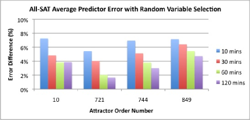
Figure 1: Average predictor error difference on melanoma attractor data using MiniSat with random variable selection modification

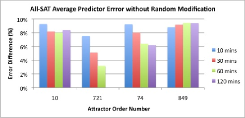
Figure 2: Average predictor error difference on melanoma attractor data using MiniSat without modification

To confirm the quality of predictor selection of our modified All-SAT, our algorithm was run on four selected attractor cycle orderings (labeled 10, 721, 744, and 849) using melanoma data from [1], allowing the All-SAT operation to run for 12 hours or until all cubes were found, whichever was first. In the case of attractor cycle order 721, all cubes were found under 12 hours. We assume that 12 hours of runtime produce predictor results closely identical to a complete All-SAT. In Figure 1 and Figure 2, we compare the average difference in predictors frequency of the 12 hour (or complete All-SAT) results with the results obtained with shorter All-SAT runtimes (of 10, 30, 60, and 120 minutes). Figure 1 shows the average error difference of all predictors for the four orderings using MiniSat with the random variable selection modification (100% random variable frequency), while Figure 2 shows the same MiniSat results without random variable selection (2% random variable frequency). For example, with attractor cycle order 721, predictor $f_{1}=\{g_{3},g_{5},g_{7}\}$ had a frequency of occurrence of 50% with a 12 hour runtime. Using random variable selection and a 30 minute runtime, the same predictor had 43% occurrence, resulting in a difference of 7%. Without random variable selection, the predictor had a 69% occurrence, a 19% error. Across the four orderings analyzed, the average error difference over all predictors (shown in Figures 1 and 2) is significantly lower using the random variable selection modification than without. At 120 minutes, the random variable selection method has a predictor occurrence that differs from true All-SAT by about 3%, while without random modification, the difference is about 8%. From this experiment, we determine that 30 minutes with random variable selection was sufficient to achieve an average of $\leq$ 5% difference from the true All-SAT results.

IV Experimental Results

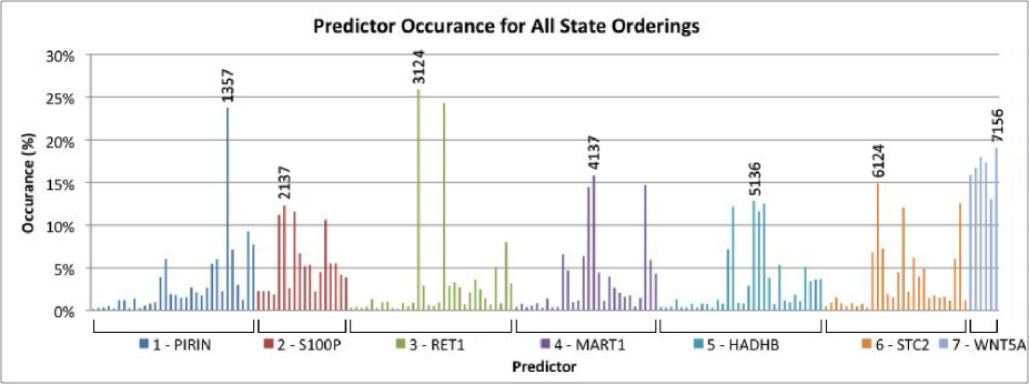
Figure 3: Method A: Predictor occurrence for all valid attractor cycle orderings (first iteration: no predictor selected)

To evaluate our SAT-based algorithm for inferring gene predictors, the algorithm was tested on gene-expression data from a melanoma study done by Bittner and Weeraratna [1]. In the melanoma study, it was observed that an abundance of RNA (expression) for gene WNT5A was associated with a high metastatis of melanoma. The study measured 587 genes with 31 gene expression patterns (lines). Seven genes are believed to be closely knit: PIRIN, S100P, RET1, MART1, HADHB, STC2, and WNT5A. There are 18 distinct patterns, which were reduced to seven using Hamming-distance of one in Table II. These seven lines form the attractor states which are the input to our algorithm.

Our algorithm utilizes a modified open-source and highly efficient exact SAT-solver called MiniSAT v1.14 [17, 7]. All-SAT operations were limited to 30 minute time-out. On average, each All-SAT run yielded 10K satisifying cubes. Our algorithm was implemented and run on a Pentium 4 Linux machine with 4GB RAM.

For the experiments, we assume two additional restrictions on attractor cycle orderings. First, we divide attractor states into good and bad states based on the presence of WNT5A. We allow good attractor states to cycle only to other good attractor states, and bad attractor states can only cycle to other bad attractor states. Second, we limit the attractor cycle length to 3 or less since long attractor cycles are highly complex and unlikely to occur in most biological systems.

In Figure 3, we display a histogram of all valid predictors and their frequency of occurrence over all attractor orderings. In this chart and table of results, a predictor label of 2367 means that gene $g_{2}$ is predicted by genes $g_{3},g_{6},$ and $g_{7}$. From this chart, we can observe that certain predictors occur with significantly higher frequency than others. For example with gene $g_{1}$, the predictor $\{x_{3},x_{5},x_{7}\}$ (PIRIN predicted by RET1, HADHB, WNT5A) occurs with much higher frequency than all other predictors for gene $g_{1}$. This indicates that this predictor is most likely to be present in the final predictor set.

From this data, we propose two methods (A and B) for selecting the predictor set. In method A, a predictor histogram is created as in Figure  3. From the histogram, for each gene $g_{i}$, we find its predictor $p^{i}_{j}$ such that:

• $p^{i}_{j}$ is the most frequently occurring predictor of gene $g_{i}$.

• The resolution ratio $R_{i}$ of this predictor (defined as the ratio of the occurrence frequency of $p^{i}_{j}$ to the occurrence frequency of the next most frequently ocurring predictor of gene $g_{i}$) is maximum.

Among all genes, we choose the one with the highest resolution ratio, and select its most frequently occuring predictor as its final predictor. After selecting this final predictor, regenerate the histogram, discarding any cubes that do not contain the final predictor(s) that have been selected in previous steps. The process repeats until all genes have a single final predictor. The set of final predictors of all genes forms the predictor set. The advantage of method A is that at every iteration, we select real predictors that have a high overall occurrence in the solution. However the method may have problems selecting final predictors if the resolution ratio is low (i.e. when the frequencies of occurrence of the predictors are nearly identical).

As an alternative, method B is proposed to determine for each gene $i$, how likely it is that gene $g_{i}$ will predict the other genes in the GRN. In other words, we ask what is the occurrence frequency of $x_{i}$ in the predictors of $f_{j}$. Table III shows how frequently a gene $g_{i}$ is used to predict a gene $g_{j}$. This table is populated by summing the occurrence frequency of all predictors of $g_{j}$ that have gene $g_{i}$ as one if their inputs. As such, any entry can be $\geq$100, and is a measure of the usefulness of $g_{i}$ as a predictor for $g_{j}$. This is done by finding, for each column $j$ of Table III, the three largest entries and adding their values. Suppose we call this value $s_{j}$ or the resolution score of column $j$. We compute the resolution score for all columns and find the final predictor the colum with the highest resolution score. This is done by listing the 3 input genes that correspond to the 3 entries that were used to compute the highest resolution score. Similar to method A, we reiterate the process by regenerating the table after discarding all cubes that do not contain predictors that were selected in previous steps. Method B has the advantage of being more robust when no single predictor has a significantly higher occurrence frequency than others. However, there is no guarantee that the predictor selected by method B is a valid predictor.

	PIRIN	S100P	RET1	MART1	HADHB	STC2	WNT5A
	$x_{1}$	$x_{2}$	$x_{3}$	$x_{4}$	$x_{5}$	$x_{6}$	$x_{7}$
BAD	0	0	0	0	0	1	1
	0	0	1	1	1	1	1
	1	0	1	0	0	0	1
GOOD	0	1	0	0	0	0	0
	0	1	1	1	0	0	0
	1	0	1	1	1	1	0
	1	1	0	1	1	0	0

TABLE II: Attractors for Melanoma Network

	$f_{1}$	$f_{2}$	$f_{3}$	$f_{4}$	$f_{5}$	$f_{6}$	$f_{7}$
$x_{1}$		59	68	57	69	60	19
$x_{2}$	24		41	29	33	49	51
$x_{3}$	65	48		76	58	56	17
$x_{4}$	39	40	78		54	44	29
$x_{5}$	56	30	27	44		39	54
$x_{6}$	42	54	52	41	44		86
$x_{7}$	64	63	24	48	32	45

TABLE III: Method B: Gene occurrence for all predictors (first iteration: no predictor selected)

In our experiments, we also use a hybrid method AB which works in the following manner. Both methods A and B are used to select their best predictor. If both methods produce the same predictor $f_{i}$, we select this predictor as a final predictor. If not, we list the best predictors for each gene for both methods. If multiple predictors match for both methods, we choose the final predictor as the one with the highest weighted sum of the resolution ratio and resolution score. The resolution ratio is weighted by 0.3 and the resolution score is weighted by 0.7. The weighting factor for resolution ratio is lower since the resolution ratio values of any gene are often close to 1. In such a situation, we would like to favor method B. If no predictor is produced by the previous step, we look at the top five predictors of method A for each gene and calculate the weighted sum of their resolution ratio and resolution score. The predictor with the highest weighted sum is selected as the final predictor. The process is reiterated, regenerating the histogram and table at each step, by discarding any cubes that do not contain any of the previously selected final predictors. With this combined approach, we are able to select predictors with a higher degree of confidence and robustness.

We ran our experiments on the melanoma attractor data of [1] using methods A, B, and AB. Results are shown in Tables IV, V, and VI respectively. Each table shows what predictor was selected at each iteration and the accompanying resolution ratio (or score). Using method A, the predictor set contains {$f_{1}=\{3,5,7\}$, $f_{2}=\{1,3,7\}$, $f_{3}=\{1,4,6\}$, $f_{4}=\{3,5,7\}$, $f_{5}=\{1,2,4\}$, $f_{6}=\{1,2,4\}$, $f_{7}=\{1,2,4\}$}. The predictor set selected by method B contains {$f_{1}=\{3,5,7\}$, $f_{2}=\{1,3,7\}$, $f_{3}=\{1,4,6\}$, $f_{4}=\{1,3,7\}$, $f_{5}=\{1,3,4\}$, $f_{6}=\{1,3,7\}$, $f_{7}=\{1,2,6\}$}. Finally, the predictor set determined through combining method A and B results in {$f_{1}=\{3,5,7\}$, $f_{2}=\{3,6,7\}$, $f_{3}=\{1,4,7\}$, $f_{4}=\{1,3,7\}$, $f_{5}=\{1,3,7\}$, $f_{6}=\{3,5,7\}$, $f_{7}=\{1,2,4\}$}.

	Iteration
	1	2	3	4	5	6	7
Predictor selected	1357	6124	3146	7124	5124	4357	2137
Resolution ratio	2.57	1.66	1.34	1.31	1.41	1.30	1.41

TABLE IV: Predictor set selection using method A

	Iteration
	1	2	3	4	5	6	7
Predictor selected	7126	3146	5134	4137	2137	1357	6137
Resolution score	2.56	1.84	1.99	1.97	1.77	1.78	1.98

TABLE V: Predictor set selection using method B

From the experiment data, we can draw several conclusive results:

• It should be noted that the final predictor set from each method is a valid satisfying cube of the SAT formula $S$. The iterative steps in regenerating the histogram (or table) retain only cubes that contain previously selected final predictors.

• The algorithm enables us to generate a few deterministic GRNs. The final predictor set is present in a select number of attractor cycle orderings. For example, the final predictor set selected by methods A, B, and AB are found in respectively 8, 4, and 6 attractor cycle orderings out of the total 5040 possible orderings.

• Some predictors are common among the predictor sets between the three methods. For example, all three methods select $f_{1}=\{g_{3},g_{5},g_{7}\}$ (PIRIN predicted by RET1, HADHB, WNT5A). We can conclude this predictor is highly likely to be a final predictor in the GRN. Also, many that are predictors selected by the three methods, while different, share common input genes. For example, the exact predictor selected by each method is different for gene $g_{2}$ (S100P), but all $f_{2}$ predictors contain 2 common genes $\{g_{3},g_{7}\}$ (RET1, WNT5A), meaning these 2 genes are likely to be contained in the final predictor of $f_{2}$.

• Using the above results, biologists can target their research on gene regulation and control, focusing on the gene relationships determined by the predictor set results.

	Iteration
	1	2	3	4	5	6	7
Predictor selected	1357	3146	4137	7124	2367	6357	5137
Resolution ratio (A)	2.57	1.07	1.11	1.57	1.28	1.77	1.01
Resolution score (B)	1.85	2.04	1.83	2.01	1.70	1.23	1.69

TABLE VI: Predictor set selection using combined method A and B

V Conclusions

Determining the predictor set for a gene regulatory network is important in many applications, particular inference and control of the GRN. In this paper, we formulate gene predictor set inference as an instance of Boolean satisfiability. In our approach, we determine all possible orderings of attractor state data, generate the CNF encapsulating predictor and biological constraints, and apply a highly-efficient and modified SAT solver to find candidate predictor sets. The SAT results are analyzed using three selection methods to produce the final predictor set. We have tested our algorithm on attractor state data from a melanoma study, and determined the predictor sets for this GRN.

Encouraged by these results, we plan to expand our SAT-based algorithm to utilize weighted max SAT. This would provide a more flexible platform where every predictor has an associated weight (or importance) in the SAT formulation. The weighted max SAT algorithm can be tailored for more restrictive biological constraints, and also would allow biologists to selectively increase or decrease weights on specific predictors. This work will incorporate the predictor set results to implement an algorithm for the inference of the complete GRN structure.

References

- [1] M. Bittner, P. Meltzer, Y. Chen, Y. Jiang, E. Seftor, M. Hendrix, M. Radmacher, R. Simon, Z. Yakhini, A. Ben-Dor, N. Sampas, E. Dougherty, E. Wang, F. Marincola, C. Gooden, J. Lueders, A. Glatfelter, P. Pollock, J. Carpten, E. Gillanders, D. Leja, K. Dietrich, C. Beaudry, M. Berens, D. Alberts, V. Sondak, N. Hayward, and J. Trent, “Molecular classification of cutaneous malignant melanoma by gene expression profiling,” Nature, vol. 406, no. 3, pp. 536–540, 2000.
- [2] W. Burke and B. M. Psaty, “Personalized Medicine in the Era of Genomics,” JAMA, vol. 298, no. 14, pp. 1682–1684, 2007.
- [3] S. M. M. Teutsch, L. A. Bradley, G. E. Palomaki, J. E. Haddow, M. Piper, N. Calonge, W. D. Dotson, M. P. Douglas, and A. O. Berg, “The evaluation of genomic applications in practice and prevention (EGAPP) initiative: methods of the EGAPP working group,” Genetics in Medicine, vol. 11, no. 1, pp. 3–14, 2009.
- [4] N. Guelzim, S. Bottani, P. Bourgine, and F. Kepes, “Topological and causal structure of the yeast transcriptional regulatory network,” Nature Genetics, vol. 31, pp. 60–63, 2002.
- [5] E. R. Dougherty, S. Kim, and Y. Chen, “Coefficient of determination in nonlinear signal processing,” Signal Processing, vol. 80, no. 10, pp. 2219 – 2235, 2000.
- [6] W. Zhao, E. Serpedin, and E. R. Dougherty, “Inferring connectivity of genetic regulatory networks using information-theoretic criteria,” IEEE/ACM Trans. Comput. Biol. Bioinformatics, vol. 5, no. 2, pp. 262–274, 2008.
- [7] “Minisat.” http://minisat.se/.
- [8] S. Kim, H. Li, E. R. Dougherty, N. Cao, Y. Chen, M. Bittner, and E. B. Suh, “Can Markov chain models mimic biological regulation?,” Journal of Biological Systems, vol. 10, no. 4, pp. 337–357, 2002.
- [9] G. Vahedi, B. Faryabi, J.-F. Chamberland, A. Datta, and E. Dougherty, “Intervention in gene regulatory networks via a stationary mean-first-passage-time control policy,” Biomedical Engineering, IEEE Transactions on, vol. 55, pp. 2319 –2331, oct. 2008.
- [10] S. A. Kauffman, “Metabolic stability and epigenesis in randomly constructed genetic nets,” Journal of Theoretical Biology, vol. 22, no. 3, pp. 437 – 467, 1969.
- [11] I. Shmulevich and E. R. Dougherty, Probabilistic Boolean Networks: The Modeling and Control of Gene Regulatory Networks. Philadelphia, PA: SIAM – Society for Industrial and Applied Mathematics, 2009.
- [12] N. Geard and J. Wiles, “A gene network model for developing cell lineages,” Artif. Life, vol. 11, no. 3, pp. 249–268, 2005.
- [13] A. Arkin, J. Ross, and H. H. McAdams, “Stochastic kinetic analysis of developmental pathway bifurcation in phage lambda-infected escherichia coli cells,” Genetics, vol. 149, pp. 1633–1648, 1998.
- [14] X. Zhou, X. Wang, and E. R. Dougherty, “Gene prediction using multinomial probit regression with Bayesian gene selection,” EURASIP Journal on Applied Signal Processing, pp. 115–124, 2004.
- [15] W. Zhou, E. Serpedin, and E. R. Dougherty, “Inferring gene regulatory networks from time series data using the minimum description length principle,” Bioinformatics, vol. 17, pp. 2129–2135, 2006.
- [16] R. Pal, I. Ivanov, A. Datta, M. L. Bittner, and E. R. Dougherty, “Generating boolean networks with a prescribed attractor structure,” Bioinformatics, vol. 21, no. 21, pp. 4021–4025, 2005.
- [17] N. Een and N. Sorensson, An Extensible SAT-solver. Lecture Notes in Computer Science, Springer Berlin / Heidelberg, 2004.