A multi-mesh finite element method for Lagrange elements of arbitrary degree

Abstract

We consider within a finite element approach the usage of different adaptively refined meshes for different variables in systems of nonlinear, time-depended PDEs. To resolve different solution behaviours of these variables, the meshes can be independently adapted. The resulting linear systems are usually much smaller, when compared to the usage of a single mesh, and the overall computational runtime can be more than halved in such cases. Our multi-mesh method works for Lagrange finite elements of arbitrary degree and is independent of the spatial dimension. The approach is well defined, and can be implemented in existing adaptive finite element codes with minimal effort. We show computational examples in 2D and 3D ranging from dendritic growth to solid-solid phase-transitions. A further application comes from fluid dynamics where we demonstrate the applicability of the approach for solving the incompressible Navier-Stokes equations with Lagrange finite elements of the same order for velocity and pressure. The approach thus provides an easy to implement alternative to stabilized finite element schemes, if Lagrange finite elements of the same order are required.

1 Introduction

Nowadays, adaptive h-methods for mesh refinement are a standard technique in finite element codes. They are used to resolve a mesh due to the local behaviour of the solution. When solving PDEs with multiple variables, e.g. velocity and pressure in the Navier-Stokes equations, the mesh has to be adapted to the behaviour of all components of the solution. If these behaviours are different, the use of a single mesh may lead to an inefficient numerical method. In this work we propose a multi-mesh finite element method that makes it possible to resolve the local nature of different components independently of each other. This method works for Lagrange elements of arbitrary degree in any dimension. Furthermore, the method works “on the top” of standard adaptive finite element methods. Hence, only small changes are required if our method has to be implemented in existing finite element codes. We have implemented the multi-mesh method in our finite element software AMDiS (adaptive multidimensional simulations), see [1], for Lagrange finite elements up to fourth degree for 1D, 2D and 3D.

To our best knowledge, Schmidt [2] was the first who has considered the use of multiple meshes in this context. Li et al. have introduced a very similar technique and used it to simulate dendritic growth [3, 4, 5]. Although introducing a multi-mesh technique, in none of these publications the method is formally derived. Furthermore implementation issues are not discussed and detailed runtime results, which compare the overall runtime between the single-mesh and the multi-mesh method are missing. In contrast, in this work we will formally show how multiple meshes are used in the context of assembling matrices and vectors in the assembly step of the finite element methods and will discuss issues related to error estimates for each component. Furthermore, we will compare the runtimes of both methods and show that the multi-mesh method is superior to the single-mesh method, when one component of the PDE can locally be resolved on a coarser mesh. Solin et al. [6, 7] have also introduced a multi-mesh method, but for hp-FEM. Their method is based on transforming quadrature points which is harder to implement in existing finite element codes. Furthermore, also in these works detailed runtime studies are missing. We should further mention other approaches which are commonly used to deal with different meshes for different components of coupled systems. Especially in the case of multi-physics applications a need exists to couple independent simulations code. A standard tool which can be used to couple various finite element codes is MpCCI (mesh-based parallel code coupling interface) [8]. In this approach an interpolation between the different solutions from one mesh to the other is performed which for different resolutions of the involved meshes will lead to a loss in information and is thus not the method of choice for the problems to be discussed in this work.

The paper is structured as follows: In the next section we give a brief overview on adaptive meshes, especially in the context of AMDiS, and introduce the terminology used throughout this paper. Section 3 introduces the so called virtual mesh assembling, which is the basis of our multi-mesh method. It is shown, how the coupling meshes are build in a virtual way and how the corresponding coupling operators are assembled on them. In Section 4, we present several numerical experiments in 2D and 3D that show the advantages of the multi-mesh method. The last section summarizes our results.

2 Adaptive meshes

The usage of an adaptive mesh, together with error estimators and a refinement strategy, is a standard finite element technique to compute solution of PDEs with a given accuracy with the lowest possible computational effort. For a general overview on this topic see for example [9], and references therein. In this section, we describe how adaptive meshes and the associated algorithms are implemented in our finite element software AMDiS. The data structures that are used to store and manipulate adaptive meshes, are the basis for a fast and efficient multi-mesh method, as it is presented in the next section.

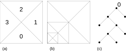
Fig. 1: (a) A two-dimensional macro mesh. (b) Some refinements of it. (c) Binary tree of macro element 0

A mesh in AMDiS consist of simplicial elements, which are lines in 1D, triangles in 2D and tetrahedral in 3D. If an element has to be refined within the adaption loop, it will be bisected into two elements of the same dimension. The refinement algorithm, that is implemented in AMDiS, is described in [10] in more detail. The two new elements are called children of the parent element. The coarsest elements are called macro elements. Accordingly, the macro mesh is the union of all macro elements. The refinement history of a macro element is represented by a binary tree. If a node in this tree is a leaf, the corresponding element is not refined. Otherwise, the children of the node represent the children of the element. To avoid hanging nodes (vertices of an element which are not vertices of the neighbour element), it may be necessary to first refine a neighbour of an element before refining the element itself. In this way, a single refinement can cause some propagation refinements of elements in the neighbourhood. In Figure 1, a triangular macro mesh consisting of four elements (a), some refinements of this macro triangulation (b) and the corresponding binary tree for macro element 0 (c) are shown.

All topological and geometrical information are only stored for the macro elements. To get these information for other elements in the mesh, an algorithm called mesh traverse is used. This algorithm traverses all binary trees, corresponding to the macro elements, and recursively computes the requested information, e.g. coordinates of vertices, for the requested child elements from the information of its parent element. The mesh traverse algorithm than calls a function that computes on the element data. An algorithm, that makes use of the mesh traverse, can specify the element level on which it wants to process. The level of an element is defined to be the depth of its node representation in the binary tree. In most cases, the leaf level, i.e., the union of all leaves in all binary trees, is used for mesh traverse.

The additional effort to compute the element data for the leaf mesh multiple times is usually less than 1% of the computational time of the function that process on the mesh. Instead, a large amount of memory can be saved. In AMDiS, the information data for one element requires around 200 bytes per element. Many of our simulations make use of around one million elements per processor. Storing all element information explicitly for these simulations would require more than 200 Mbyte of extra memory.

2.1 Error estimation and adaptive strategies

AMDiS provides different methods for error estimation and mesh refinement. Furthermore, due to an abstract interface, is is easily possible to implement other methods, that are more adapted to a specific PDE. In the following, we describe the most common ones.

In AMDiS, the standard estimator for the spatial error is the residual error estimator as for example described by Verfürth [11] for general non-linear elliptic PDEs. This local element wise estimator defines for each element $T$ of a mesh an indicator, depending on the finite element solution $u_{h}$, by

$$\eta_{T}(u_{h})=C_{o}R_{T}(u_{h})+C_{1}\sum_{E\subset T}J_{E}(u_{h}),$$ (1)

where $R_{T}$ is the element residual on element $T$ and $J_{E}$ is the jump residual, defined on an edges $E$. $C_{0}$ and $C_{1}$ are user defined constants that can be used to adjust the estimator. The global error estimation of a finite element solution is than the sum of the local estimates:

$$\eta(u_{h})=\left(\sum_{T\in{\cal T}}\eta_{T}(u_{h})^{p}\right)^{1/p},\hskip 28.45274ptp\geq 1,$$ (2)

where ${\cal T}$ is a partitions of the domain into simplices. The user has to specify an error tolerance $tol$. If $\eta(u_{h})>tol$, the mesh must be refined in some way in order to reduce the error. Several strategies are implemented in AMDiS:

• the maximum strategy, as described by Verfürth [12],

• the equidistribution strategy, as described by Eriksson and Johnson [13],

• the guaranteed error reduction strategy, as described by Dörfler [14].

In all of the numerical experiments in Section 4, we make use of the equidistribution strategy, which we found out to be easy to use and which provided good results. The basis for this strategy is the idea that the error is assumed to be equidistributed over all elements. Hence, if the partition consists of $n$ elements, the element error estimates should fulfill

$$\eta_{T}(u_{h})\approx\frac{tol}{n^{1/p}}\equiv\eta_{eq}(u_{h}).$$ (3)

The equidistribution strategy now introduces two parameters, $\theta_{R}\in(0,1)$ and $\theta_{C}\in(0,1)$. An element is refined, if $\eta_{T}(u_{h})>\theta_{R}\eta_{eq}(u_{h})$, and the element is coarsen, if $\eta_{T}(u_{h})\leq\theta_{C}\eta_{eq}(u_{h})$. The parameter $\theta_{R}$ is usually chosen to be close to 1, and $\theta_{C}$ to be close to 0, respectively.

If the equation consists of more than one variable, one can define multiple error estimators and mesh adaption strategies. This is also the case, if only one mesh is used to resolve all variables. The error estimators work independently of each other, and the user can provide the constants $C_{0}$ and $C_{1}$ for each component. Correspondingly, independent mesh adaption strategies may be defined for each component. In the case of the single-mesh method, an element is refined, if at least one strategy has marked the element to be refined. An element is coarsen, if all strategies have marked it to be coarsen. In the multi-mesh method, these conditions are omitted, because the meshes are adapted independently of each other.

3 Virtual mesh assembling

The basis of our multi-mesh method is the so called virtual mesh assembling. Systems of PDEs usually involve coupling terms. If each component of the system is assembled on a different mesh, special care has to be devoted to these coupling terms. In the next section, we shortly describe this situation. The section 3.2 than introduces the dual mesh traverse. This algorithm create a virtual union of two meshes without creating it explicitly. To the last, we show how to compute integrals, that appear within the assemble procedure, on these virtual meshes.

3.1 Coupling terms in systems of PDEs

To illustrate the techniques presented in this section, we consider the homogeneous biharmonic equation as a simple example for general systems of PDEs. This equation reads:

$$\Delta^{2}u=0\;\;\text{in}\;\;\Omega\hskip 14.22636pt\text{and}\hskip 14.22636ptu=\frac{\partial u}{\partial n}=0\;\;\text{on}\;\;\partial\Omega,$$ (4)

with $u\in C^{4}(\Omega)\>\cap\>C^{1}(\bar{\Omega})$. Using operator splitting, the biharmonic equation can be rewritten as a system of two second order elliptic PDEs:

$$\begin{split}-\Delta u+v&=0\\ \Delta v&=0\end{split}$$ (5)

The standard mixed variational formulation of this system is: Find $(u,v)\in H_{0}^{1}(\Omega)\times H^{1}(\Omega)$ such that

$$\begin{split}\int_{\Omega}\nabla u\nabla\phi dx+\int_{\Omega}v\phi dx&=0\hskip 28.45274pt\forall\phi\in H^{1}(\Omega)\\ \int_{\Omega}\nabla v\nabla\psi dx&=0\hskip 28.45274pt\forall\psi\in H_{0}^{1}(\Omega)\end{split}$$ (6)

To discretize these equations, we assume that ${\cal T}_{h}^{0}$ and ${\cal T}_{h}^{1}$ are different partitions of the domain $\Omega$ into simplices. Than, $V_{h}^{0}=\{v_{h}\in H^{1}:v_{h}|_{T}\in P^{n}\;\forall T\in{\cal T}_{h}^{0}\}$ and $V_{h}^{1}=\{v_{h}\in H_{0}^{1}:v_{h}|_{T}\in P^{n}\;\forall T\in{\cal T}_{h}^{1}\}$ are finite element spaces of globally continuous, piecewise polynomial functions of an arbitrary but fixed degree. We thus obtain: Find $(u_{h},v_{h})\in V_{h}^{0}\times V_{h}^{1}$ such that

$$\begin{split}\int_{\Omega}\nabla u_{h}\nabla\phi dx+\int_{\Omega}v_{h}\phi dx&=0\hskip 28.45274pt\forall\phi\in V_{h}^{0}(\Omega)\\ \int_{\Omega}\nabla v_{h}\nabla\psi dx&=0\hskip 28.45274pt\forall\psi\in V_{h}^{1}(\Omega).\end{split}$$ (7)

Let define $\{\phi_{i}\mid 1\leq i\leq n\}$ and $\{\psi_{i}\mid 1\leq i\leq m\}$ to be the nodal basis of $V_{h}^{0}$ and $V_{h}^{1}$, respectively. Hence, $u_{h}$ and $v_{h}$ can be written by the linear combinations $u_{h}=\sum_{i=1}^{n}u_{i}\phi_{i}$ and $v_{h}=\sum_{i=1}^{m}v_{i}\psi_{i}$, with $u_{i}$ and $v_{i}$ the unknown real coefficients. Using these relations and braking up the domain in the partitions of $\Omega$, Equation (7) rewrites to

$$\begin{split}\sum_{j=1}^{n}u_{j}\left(\sum_{T\in{\cal T}^{0}_{h}}\int_{T}\nabla\phi_{j}\cdot\nabla\phi_{i}\right)+\sum_{j=1}^{m}v_{j}\left(\sum_{T\in{\cal T}^{0}_{h}\cup{\cal T}^{1}_{h}}\int_{T}\psi_{j}\phi_{i}\right)&=0\hskip 21.33955pti=1\dots n\\ \sum_{j=1}^{m}v_{j}\left(\sum_{T\in{\cal T}^{1}_{h}}\int_{T}\nabla\psi_{j}\cdot\nabla\psi_{i}\right)&=0\hskip 21.33955pti=1\dots m.\\ \end{split}$$ (8)

To compute the coupling term, we have to define the union of two different partitions $T_{h}^{0}\cup T_{h}^{1}$. For this, we make a restriction on the partitions: Any element $T^{0}\in{\cal T}_{h}^{0}$ is either a subelement of an element $T^{1}\in{\cal T}_{h}^{1}$, or vice versa. This restriction is not very strict. It is always fulfilled for the standard bisectioning algorithm, if the initial meshes for all components share the same macro mesh. Then, ${\cal T}^{0}_{h}\cup{\cal T}^{1}_{h}$ is the union of the locally finest simplices.

The most common way to compute the integrals in Equation (8) is to define local basis functions. We define $\phi_{i,j}$ to be the $j$-th local basis function on an element $T_{i}\in{\cal T}^{0}_{h}$. $\psi_{i,j}$ is defined in the same way for elements in the partition ${\cal T}^{1}_{h}$.

Because the global basis functions $\phi_{i}$ and $\psi_{j}$ are defined on different triangulations of the same domain, it is not straightforward to calculate the coupling term $\int_{\Omega}\psi_{j}\phi_{i}$ in an efficient manner. For evaluating this integral, two different cases may occur: either the integral has to be evaluated on an element from the partition ${\cal T}^{0}_{h}$ or on an element from ${\cal T}^{1}_{h}$. For what follows, we fix the first case. In terms of local basis functions we have to evaluate

$$\int_{T_{i}\in{\cal T}^{0}_{h}}\psi_{k,l}\phi_{i,j}$$ (9)

for some $j$ and $l$, and there exists an element $T_{k}\in{\cal T}^{1}_{h}$, with $T_{i}\subset T_{k}$. Our aim is to develop a multi-mesh method that works on the top of existing finite element software. These have usually implemented special methods to evaluate local basis functions, or the multiplication of two basis functions, respectively, on elements very fast. This involves for example precalculated integral tables or fast quadrature rules. All these methods cannot directly be applied to the coupling terms, because $\psi_{k,l}$ in Equation (9) is not a local basis function of the element $T_{i}$. The general idea to overcome this problem is to define the basis functions $\psi_{k,l}$ by a linear combination of local basis functions of $T_{i}$. Thus,

$$\int_{T_{i}\in{\cal T}^{0}_{h}}\psi_{k,l}\phi_{i,j}=\int_{T_{i}\in{\cal T}^{0}_{h}}\sum_{m}(c_{k,m}\phi_{i,m})\phi_{i,j},$$ (10)

with some real coefficients $c_{k,m}$. For the other case, i.e., the integral in the coupling term is evaluated on an element $T_{i}\in{\cal T}^{1}_{h}$, we have

$$\int_{T_{i}\in{\cal T}^{1}_{h}}\psi_{k,l}\phi_{i,j}=\int_{T_{i}\in{\cal T}^{1}_{h}}\psi_{k,l}\sum_{m}(c_{i,m}\psi_{k,m}).$$ (11)

Summarized, to make evaluate of the coupling terms possible, two different techniques have to be defined and implemented: Firstly, the method requires to build a union of two meshes. This leads to an algorithm which we name dual mesh traverse. It will be discussed in the next section. Once the union is obtained, we need to calculate the coefficients $c_{i,j}$ and to incorporate them in the finite element assemblage procedure such that the overall change of the standard method is as small as possible.

3.2 Creation of the virtual mesh

The simplest way to obtain the union of two meshes is to employ the data structure they are stored in. Hence, in our case we could explicitly build the union by joining the binary trees of both meshes into a set of new binary trees. Especially when we consider meshes that change in time, this procedure is not only too time-consuming but requires also additional memory to store the joined mesh. To avoid this, we exploit the case that in AMDiS functions, that process element data, never directly work on the mesh data but instead use the mesh traverse algorithm, that creates the requested element data on demand. According to this method, we define the dual mesh traverse that traverses two meshes in parallel and thus creates the union of both meshes in a virtual way.

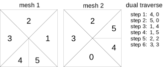
Fig. 2: Dual mesh traverse on two independent refined meshes on the same macro mesh.

For the dual mesh traverse the only requirement is that both meshes must share the same macro mesh, but they can be refined independently of each other. Due to this requirement and because of the bisectioning refinement algorithm the following holds: If the intersection of two elements of two different meshes is non empty, then either both elements are equal or one element is a real subelement of the other. To receive the leaf level of the virtual mesh, the dual mesh traverse simultaneously traverses two binary trees, each corresponding the the same macro element in both macro meshes. The algorithm than calls a user defined function, e.g. the element assembling function or an element wise error estimator, that works on pairs of elements, with both, the larger and the smaller element of the current traverse. The larger of both elements is fixed as long as all smaller subelements in the other mesh are traversed. Figure 2 shows a simple example for a macro mesh consisting of four macro elements. In the first mesh macro element 0, and in the second mesh macro element 1 are refined once.

3.3 Assembling of element matrices

To make the overall calculation as fast as possible, the form as given by the Equations (10) and (11) is not appropriate. To implement these transformations, some changes of the inner assemblage procedure would be required. In the following, we show in which way the transform matrices can be incorporated in the standard assemble procedure, such that the changes will be as small as possible. To the first, we have to distinguish two cases: the smaller of both elements defines either the space of test functions, or it defines the space of trial functions. For the first case, assume a general zero order term of the form $\int_{\Omega}\psi_{i}c\phi_{j}$, with $c\in L^{\infty}(\Omega)$ and some local basis functions $\psi_{i}$ and $\phi_{j}$, has to be assembled on a virtual mesh. Then, for some elements $T$ and $T^{\prime}$, with $T^{\prime}\subset T$, the element matrix $M_{T^{\prime}}$ is given by

$$\begin{split}M_{T^{\prime}}&=\begin{pmatrix}\int_{T^{\prime}}\psi_{0}c\phi_{0}&\dots&\int_{T^{\prime}}\psi_{0}c\phi_{n}\\ \vdots&&\vdots\\ \int_{T^{\prime}}\psi_{n}c\phi_{0}&\dots&\int_{T^{\prime}}\psi_{n}c\phi_{n}\end{pmatrix}\\ &=\begin{pmatrix}\int_{T^{\prime}}\sum_{i}(c_{0i}\phi_{i})c\phi_{0}&\dots&\int_{T^{\prime}}\sum_{i}(c_{0i}\phi_{i})c\phi_{n}\\ \vdots&&\vdots\\ \int_{T^{\prime}}\sum_{i}(c_{ni}\phi_{i})c\phi_{0}&\dots&\int_{T^{\prime}}\sum_{i}(c_{ni}\phi_{i})c\phi_{n}\end{pmatrix}\\ &=\begin{pmatrix}\sum_{i}c_{0i}\int_{T^{\prime}}\phi_{i}c\phi_{0}&\dots&\sum_{i}c_{0i}\int_{T^{\prime}}\phi_{i}c\phi_{n}\\ \vdots&&\vdots\\ \sum_{i}c_{ni}\int_{T^{\prime}}\phi_{i}c\phi_{0}&\dots&\sum_{i}c_{ni}\int_{T^{\prime}}\phi_{i}c\phi_{n}\end{pmatrix}\\ &={\cal C}\cdot\begin{pmatrix}\int_{T^{\prime}}\phi_{0}c\phi_{0}&\dots&\int_{T^{\prime}}\phi_{0}c\phi_{n}\\ \vdots&&\vdots\\ \int_{T^{\prime}}\phi_{n}c\phi_{0}&\dots&\int_{T^{\prime}}\phi_{n}c\phi_{n}\end{pmatrix},\end{split}$$ (12)

where $\phi_{i}$ are the local basis function defined on $T^{\prime}$, $\psi_{i}$ are the local basis function defined on $T$, and ${\cal C}$ is the transformation matrix for the local basis function from $T$ to $T^{\prime}$. This shows, that to assemble the element matrix of a virtual element, there is no need for larges changes within the assemble procedure. The finite element code needs only to assemble the element matrix of the smaller element $T^{\prime}$ and multiply the result with the transformation matrix. Hence, if the transformation matrices can be computed easily, the overhead for virtual element assembling can be neglected.

The second case, where the smaller element defines the space of trial functions, is very similar. The same calculation as above shows that the following holds:

$$M_{T^{\prime}}=\begin{pmatrix}\int_{T^{\prime}}\phi_{0}c\phi_{0}&\dots&\int_{{\cal T}^{\prime}}\phi_{0}c\phi_{n}\\ \vdots&&\vdots\\ \int_{T^{\prime}}\phi_{n}c\phi_{0}&\dots&\int_{T^{\prime}}\phi_{n}c\phi_{n}\end{pmatrix}\cdot{\cal C}^{T}$$ (13)

In a similar way we can also reformulate the element matrices for general first and second order terms. For a general second order term of the form $\int_{\Omega}\nabla\psi_{i}\cdot{\bf A}\nabla\phi_{j}$, with ${\bf A}:\Omega\mapsto\mathbb{R}^{d\times d}$, the element matrix $M_{T^{\prime}}$ can be rewritten in the same way as we have done it in (12) for general zero order terms:

$$\begin{split}M_{{\cal T}^{\prime}}&=\begin{pmatrix}\int_{{\cal T}^{\prime}}\nabla\psi_{0}\cdot{\bf A}\nabla\phi_{0}&\dots&\int_{{\cal T}^{\prime}}\nabla\psi_{0}\cdot{\bf A}\nabla\phi_{n}\\ \vdots&&\vdots\\ \int_{{\cal T}^{\prime}}\nabla\psi_{n}\cdot{\bf A}\nabla\phi_{0}&\dots&\int_{{\cal T}^{\prime}}\nabla\psi_{n}\cdot{\bf A}\nabla\phi_{n}\end{pmatrix}\\ &={\cal C}_{\nabla}\cdot\begin{pmatrix}\int_{{\cal T}^{\prime}}\nabla\phi_{0}\cdot{\bf A}\nabla\phi_{0}&\dots&\int_{{\cal T}^{\prime}}\nabla\phi_{0}\cdot{\bf A}\nabla\phi_{n}\\ \vdots&&\vdots\\ \int_{{\cal T}^{\prime}}\nabla\phi_{n}\cdot{\bf A}\nabla\phi_{0}&\dots&\int_{{\cal T}^{\prime}}\nabla\phi_{n}\cdot{\bf A}\nabla\phi_{n}\end{pmatrix}\\ \end{split}$$ (14)

where the coefficients of the matrix ${\cal C}_{\nabla}$ are defined such that

$$\nabla\psi_{i}=\sum_{j=0}^{n}c_{ij}\nabla\phi_{i}.$$ (15)

If the smaller element defines the space of trial functions, we can establish the same relation as in (13). For general first order terms of the form $\int_{\Omega}\psi_{i}{\bf b}\cdot\nabla\phi_{j}$, with ${\bf b}\in[L^{\infty}(\Omega)]^{d}$, it is simple to check that for the case the smaller element defines the test space, the element matrix $M_{T^{\prime}}$ can be calculated on the smaller element and multiplied with ${\cal C}$ from the left. If the smaller element defines the space of trial function, the element matrix calculated on the smaller element must be multiplied with ${\cal C}_{\nabla}^{T}$ from the right.

3.4 Calculation of transformation matrices

We have shown that if the transformation matrix is calculated for a given tuple of small and large element, the additional cost for virtual mesh assembling is very small. In this section, we show how to compute these transformation matrices efficiently. We formally define a virtual element pair by the tuple

$$(T,\{\alpha_{0},\text{\ldots},\alpha_{n}\})=(T,\alpha)\>\text{with}\>\alpha_{i}\in\{\text{L},\text{R}\},$$ (16)

where $T$ is the larger element of the pair and $\alpha$ is an ordered set that is interpreted as the refinement sequence for element $T$. Thus, L denotes the “left”, and R denotes the “right” children of and element. Furthermore, we define a function $TRA$ that uniquely maps a virtual element pair to the smaller element. It is defined recursively by:

$$TRA(T,\emptyset) = T$$

$$TRA(T,\{\alpha_{0},\alpha_{1},\text{\ldots},\alpha_{n}\}) = \begin{cases}TRA(T_{\text{L}},\{\alpha_{1},\text{\ldots},\alpha_{n}\})&\text{if}\>\alpha_{0}=\text{L}\\ TRA(T_{\text{R}},\{\alpha_{1},\text{\ldots},\alpha_{n}\})&\text{if}\>\alpha_{0}=\text{R},\end{cases}$$

where $T_{\text{L}}$ is the left child of the element $T$, and $T_{\text{R}}$ the right child of the element, respectively. In the same way we can now define transformation matrices as functions on refinement sequences:

$${\cal C}(\emptyset) =$$ I

$${\cal C}(\{\alpha_{0},\alpha_{1},\text{\ldots},\alpha_{n}\}) = \begin{cases}{\cal C}_{\text{L}}\cdot{\cal C}(\{\alpha_{1},\text{\ldots},\alpha_{n}\})&\text{if}\>\alpha_{0}=\text{L}\\ {\cal C}_{\text{R}}\cdot{\cal C}(\{\alpha_{1},\text{\ldots},\alpha_{n}\})&\text{if}\>\alpha_{0}=\text{R},\end{cases}$$

where ${\cal C}_{L}$ and ${\cal C}_{R}$ are the transformation matrix for the left child and the right child, respectively, of the reference element.

3.5 Implementation issues

Although the calculation of transformation matrices is quite fast, it can considerably increase the time for assembling the linear system. This is especially the case, if one mesh is much coarsen in some regions than the other mesh. To circumvent this problem, we have implemented a cache, that stores the transformation matrices. In the mesh traverse routine, an 64 bit integer data type stores the refinement sequence bit-wise, as it is defined by (16). If the bit on the i-th position is set, the finer element is a right-refinement of its parent element, otherwise it is a left-refinement of it. Of coarse this limits the level gap between the coarser and the finer level to be less or equal to 64. But we have not found any practical simulations, where this value is more than 30. Using this data type makes it than easy to define associative array that uniquely maps a refinement sequence to a transformation matrices. If a transformation matrix was computed for a given refinement sequence for the first time, it will be stored in this array. To access previously computed matrices using the integer key is than very cheap. In general this data structure should be restricted to a fixed number of matrices to not spend to much of memory. In all of our simulations, the number of matrices that should be stored in the cache never exceed 100.000. Also in the 3D case with linear elements the overall memory usage is than around 2 Mbyte, and can thus be neglected. Therefore, we have not yet considered to implement an upper limit for the cache.

4 Numerical results

In this section, we present several examples, where the multi-mesh approach is superior in contrast to the standard single-mesh finite element method. Examples to be considered are phase-field equations to study solid-liquid and solid-solid phase transitions. For a recent review we refer to [15]. These equations involve at least one variable, the phase-field variable, which is almost constant in most parts of the domain and thus can be discretized within these parts using a coarse mesh. Within the interface region however a high resolution is required to resolve the smooth transition between the different phases. A second variable in such systems is typically a diffusion field which in most cases varies smoothly across the whole domain and thus will require a finer mesh outside of the interface and a coarser mesh within the interface. Such problems are therefor well suited for our multi-mesh approach. We will consider dendritic growth in solidification and coarsening phenomena in binary alloys to demonstrate the applicability.

Other examples for which large computational savings due to the use of the multi-mesh approach are expected are diffuse interface and diffuse domain approximations for PDE’s to be solved on surfaces are within complicated domains. The approaches introduced in [16] and [17], respectively, use a phase-field function to implicitly describe the domain the PDE has to be solved on. For the same reason as in phase-transition problems the distinct solution behaviour of the different variables will lead to large savings if the multi-mesh approach is applied. The approach has already been used for applications such as chaotic mixing in microfluidics [18], tip splitting of droplets with soluble surfactants [19], and chemotaxis of stem cells in 3D scaffolds [20].

As a further example we demonstrate that the multi-mesh approach can also be used to easily fulfill the inf-sup condition for saddle-point problems if both components are discretized using linear Lagrange elements. We demonstrate this numerically for the incompressible Navier-Stokes equation with piecewise linear elements for velocity and pressure, but a finer mesh used for the velocity. Such an approach might be superior to mixed finite elements of higher order or stabilized schemes in terms of computational efficiency and implementational efforts. For a review on efficient finite element methods for the incompressible Navier-Stokes equation we refer to [21]. We demonstrate the applicability of the multi-mesh approach on the classical driven cavity problem.

4.1 Dendritic growth

We first consider dendritic growth using a phase-field model, which today is the method of choice to simulate microstructure evolution during solidification. For reviews we refer to [22]. A widely used model for quantitative simulations of dendritic structures was introduced by Karma and Rappel [23, 24], which reads in non-dimensional from

$$\begin{split}A^{2}(n)\partial_{t}\phi&=(\phi-\lambda u(1-\phi^{2}))(1-\phi^{2})+\nabla(A^{2}(n)\nabla\phi)+\sum_{i=1}^{d}\partial_{x_{i}}\left(|\nabla\phi|^{2}A(n)\frac{\partial A(n)}{\partial_{x_{i}}\phi}\right)\\ \partial_{t}u&=D\nabla^{2}u+\frac{1}{2}\partial_{t}\phi,\end{split}$$ (17)

where $d=2,3$ is the dimension, $D$ is the thermal diffusivity constant, $\lambda=\frac{D}{a_{2}}$, with $a_{2}=0.6267$ is a coupling term between the phase-field variable $\phi$ and the thermal field $u$ and $A$ is an anisotropy function. For both, simulation in 2D and 3D, we use the following anisotropy function:

$$A(n)=(1-3\epsilon)\left(1+\frac{4\epsilon}{1-3\epsilon}\frac{\sum_{i=1}^{d}\phi_{x_{i}}^{4}}{|\nabla\phi|^{4}}\right),$$ (18)

where $\epsilon$ controls the strength of the anisotropy and $n=\frac{\nabla\phi}{|\nabla\phi|}$ denotes the normal to the solid-liquid interface. In this setting the phase-field variable is $-1$ in liquid and $1$ in solid, and the melting temperature is set to be zero. As boundary condition we set $u=-\Delta$ to specify an undercooling. For the phase-field variable we use zero-flux boundary conditions.

To implement these equations in our toolbox AMDiS, we first discretize in time. This is here done using a semi-implicit Euler method, which yields a sequence of nonlinear elliptic PDEs:

$$\begin{split}\frac{A^{2}(n_{n})}{\tau}\phi_{n+1}+f+g-\nabla(A^{2}(n_{n})\nabla\phi_{n+1})-{\cal L}[A(n_{n})]&=\frac{A^{2}(n_{n})}{\tau}\phi_{n}\\ \frac{u_{n+1}}{\tau}-D\nabla^{2}u_{n+1}-\frac{1}{2}\frac{\phi_{n+1}}{\tau}&=\frac{u_{n}}{\tau}-\frac{1}{2}\frac{\phi_{n}}{\tau}.\end{split}$$ (19)

with $f=\phi_{n+1}^{3}-\phi_{n+1}$, $g=\lambda(1-\phi_{n+1}^{2})^{2}u_{n+1}$ and

$${\cal L}[A(n_{n})]=\sum_{i=1}^{d}\partial_{x_{i}}\left(|\nabla\phi_{n+1}|^{2}A(n_{n})\frac{\partial A(n_{n})}{\partial_{x_{i}}\phi_{n}}\right).$$

We now linearize the involved nonlinear terms $f$ and $g$:

$$\begin{split}f&\approx(3\phi_{n}^{2}-1)\phi_{n+1}-2\phi_{n}^{3}\\ g&\approx\lambda(1-\phi_{n}^{2})^{2}u_{n+1}\end{split}$$ (20)

and obtain a linear system for $\phi_{n+1}$ and $u_{n+1}$ to be solved in each time step.

To compare our multi-mesh method with a standard adaptive finite element approach, we have computed a dendrite using linear finite elements. The following parameters are used:

$$\Delta=0.65,D=1.0,\epsilon=0.05$$

We have run the simulation with a constant timestep $\tau=1.0$ up to time $7500$. To speedup the computation we have employed the symmetry of the solution and limited the computation to the upper right quadrant with a domain size of 800 into each direction. The adaptive mesh refinement relies on the residuum based a posteriori error estimate, as defined by 1. By setting $C_{0}$ to 0 and $C_{1}$ to 1, we restrict the estimator to the jump residuum only. We have set the tolerance to be $tol_{\phi}=0.5$ and $tol_{u}=0.25$. For adaptivity, the equidistribution strategy with parameters $\theta_{R}=0.8$ and $\theta_{C}=0.2$ was used. Thus, the interface is resolved by around 20 points.

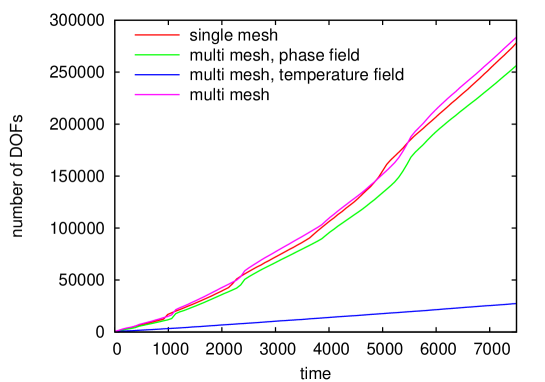
Fig. 3: Evolution of degrees of freedom in time for the phase field and the temperature field using single-mesh and multi-mesh method.

The result of both computations coincides at the final timestep. As a quantitative comparison we use the tip velocity of the dendrite. As reported by Karma and Rappel [24], for this parameter set analytical calculations lead to a steady-state tip velocity $V_{tip}=0.0469$. In both of our calculations, the tip velocity varies around 1% to this value. Using the single-mesh method, within the final timestep the mesh consist of 278.252 degrees of freedom (DOFs). When our multi-mesh method is used, the same solution can be obtained with a mesh for the phase-field with 256.342 DOFs and 27.354 DOFs for the temperature field. The gap between these numbers increase over time, see Figure 3 showing the development of DOFs over time. Figure 4 qualitatively compares the meshes of the phase-field variable and the temperature field which shows the expected finer resolution of the phase-field mesh within the interface and its coarser resolution within the solid and liquid region.

The computational time for both methods is compared in Table 1. The assemblage procedure in the multi-mesh methods is around 6% faster, although computing the element matrices is slower due to the extra matrix-matrix multiplication. This is easily explained by the fact that we have much less element matrices to compute and the overall matrix data structure is around 50% smaller with respect to the number of non-zero entries. This is also reflected in the solution time for the linear system. We have run all computation twice, with using either UMFPACK, a multifrontal sparse direct solver [25], or the BiCGStab($\ell$) with diagonal preconditioning, that is part of the Math Template Library (MTL4), see [26]. When using the first one within the multi-mesh method, the solution time can be reduced by 40% and also the memory usage, which is often the most critical limitation in the usage of direct solvers, is reduced in this magnitude. An even more drastic reduction of the computation time can be achieved when using an iterative solver. Here, the number of iterations is around 30% less with the multi-mesh method and each iteration is faster due to the smaller matrix. The time for error estimation is halved, as expected, since it scales linearly with the number of elements in the mesh. Altogether, the time reduction is significant in all parts of the finite element method for this example. In addition the approach also leads to a drastic reduction in the memory usage.

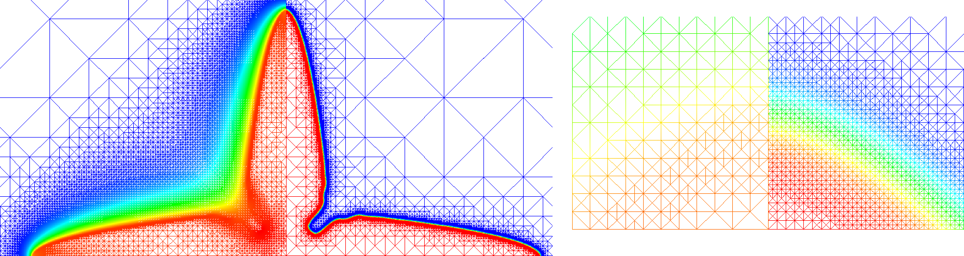
Fig. 4: a) 2D dendrite computed at $t=7500$ using the multi-mesh method with the parameters $\Delta=0.65$, $D=1.0$, $\epsilon=0.05$ and a timestep $\tau=1.0$. Left shows the mesh of the temperature field and right shows the mesh of the phase field. b) Zoom into the upper tip showing the different resolution of both meshes.

	single-mesh	multi-mesh	speedup
assembler	5.98s	5.62s	6.0%
solver: UMFPACK	6.69s	4.12s	38.4%
solver: BiCGStab$(\ell)$	14.26s	4.28s	69.9%
estimator	3.40s	1.71s	49.7%
overall with UMFPACK	16.07s	11.45s	28.7%
overall with BiCGStab$(\ell)$	23.64s	11.61s	50.9%

Table 1: Comparison of runtime when using single-mesh and multi-mesh method. The values are the average of 7500 timesteps.

The results are even more significant in 3D. Figure 5 shows the result of computing a dendrite with the multi-mesh method and the following parameters:

$$\Delta=0.55,D=1,\epsilon=0.05$$

We have run the simulation with a constant timestep $\tau=1.0$ up to time 2500. The evolution of degrees of freedom over time is quite similar to the 2D example. When using the multi-mesh method, the time for solving the linear system, again using the BiCGStab($\ell$) solver with diagonal preconditioning, can be reduced by around 60%. The time for error estimation is around half the time needed by the single-mesh method. Because the time for assembling the linear system is more significant in 3D, the overall time reduction with the multi-mesh method is around $24.4\%$.

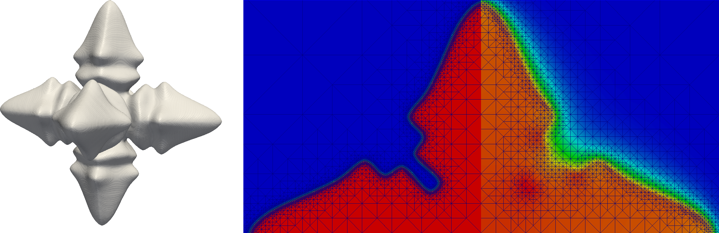
Fig. 5: a) 3D dendrites at t = 2500 using the multi-mesh method with the parameters $\Delta=0.55$, $D=1$, $\epsilon=0.05$ and a timestep $\tau=1.0$. b) Slice through the dendrites showing the mesh of the phase field on the left and the mesh of the temperature field on the right hand side.

4.2 Coarsening

As a second example we consider coarsening of a binary structure using a Cahn-Hilliard equation. We here concentrate only on the phenomenological behaviour of the solution and thus consider the simplest isotropic model, which reads

$$\begin{split}\partial_{t}\phi&=\Delta\mu\\ \mu&=-\epsilon\Delta\phi+\frac{1}{\epsilon}G^{\prime}(\phi)\end{split}$$ (21)

for a phase-field function $\phi$ and a chemical potential $\mu$. The parameter $\epsilon$ again defines a length scale over which the interface is smeared out, and $G(\phi)=18\phi^{2}(1-\phi)^{2}$ defines a double-well potential. To discretize in time we again use a semi-implicit Euler scheme

$$\begin{split}\frac{1}{\tau}\phi_{n+1}-\Delta\mu_{n+1}&=\frac{1}{\tau}\phi_{n}\\ \mu_{n+1}+\epsilon\Delta\phi_{n+1}-\frac{1}{\epsilon}G^{\prime}(\phi_{n+1})&=0\end{split}$$ (22)

in which we linearize $G^{\prime}(\phi_{n+1})\approx G^{\prime\prime}(\phi_{n})\phi_{n+1}+G^{\prime}(\phi_{n})-G^{\prime\prime}(\phi_{n})\phi_{n}$.

To compare our multi-mesh method with a standard adaptive finite element approach, we have computed the spinodal decomposition and coarsening process using Lagrange finite elements of fourth order. We use $\epsilon=5\cdot 10^{-4}$. The adaptive mesh refinement relies on the residuum based a posteriori error estimate. As we have done it in the dendritic growth simulation, also here only the jump residuum is considered, i.e., the constants $C_{0}$ and $C_{1}$ in Equation (1) are set to 0 and 1, respectively. For both methods, the error tolerance are set to $tol_{\phi}=2.5\cdot 10^{-4}$ and $tol_{\mu}=5\cdot 10^{-2}$. For adaptivity, the equidistribution strategy with parameters $\theta_{R}=0.8$ and $\theta_{C}=0.2$ was used. Using these parameters, the interface is resolved by around 10 points.

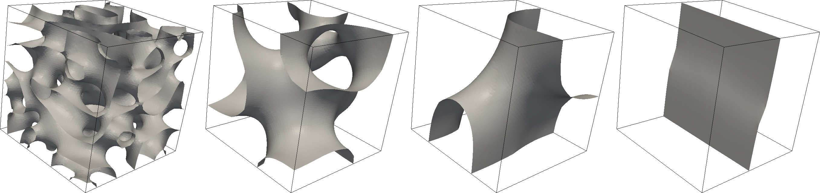
Fig. 6: Solution of the Cahn-Hilliard equation for $t=0.02$, $t=1.0$, $t=5.0$ and $t=12.50$

The simulation was started from noise. The first mesh was globally refined with 196608 elements. The constant timestep was chosen to be $\tau=10^{-3}$. We have disabled the adaptivity for the first 10 timesteps, until a very first coarsening in the domain was achieved. Then the simulation was executed up to $t=13.0$, where both phases are nearly separated. Figure 6 shows the phase field, i.e., the 0.5 contour of the first solution variable, for four different timesteps. The number of elements and degrees of freedom is linear to the area of the interface that must be resolved on the domain. Indeed, the chemical potential can be resolved on a mush coarser grid, since it is independent of the resolution of the phase field. In the final state, the chemical potential is constant on the whole domain, and the macro mesh (which consists of 6 elements in this simulation) is enough to resolve it. The evolution of the number of elements for both variable over time is plotted in Figure 7. As expected, the number of elements for the phase field monotonously decreases as its area shrinks due to the coarsening process. The number of elements for the chemical potential rapidly decreases at the very first beginning, as the initial mesh is over refined to resolve this variable. For most of the simulation, the number of elements of the chemical potential is three magnitudes smaller the the number of elements for the phase field variable. This gap is also reflected in the computation time for the single-mesh and the multi-mesh method. AMDiS has computed the solution with the multi-mesh method in 722 minutes. When using the standard single-mesh method, where the number of elements for the only mesh is nearly equivalent to the number of elements needed in the phase field mesh when using the multi-mesh approach, the simulation time was 1465 minutes. For both simulations, we have used the BiCGStab$(\ell)$ solver with diagonal preconditioning.

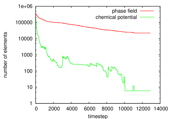
Fig. 7: Evolution of number of elements for both variables of the Cahn-Hilliard equation.

4.3 Fluid dynamics

For the last example, we use our multi-mesh method to solve problems in fluid dynamics using standard linear finite elements. The inf-sub stability is established by using two different meshes. In 2D, the mesh for the velocity components is refined twice more than the mesh for pressure. In the 3D case, the velocity mesh has to be refined three times to get the corresponding refinement structure. This discretization was introduced by Bercovier and Pironneau [27], and was analyzed and proven to be stable by Verfürth [28]. To show this technique, we solve the standard instationary Navier-Stokes equation given by

$$\begin{split}\partial_{t}u-\nu\nabla^{2}u+u\cdot\nabla u+\nabla p&=f\\ \nabla\cdot u&=0,\end{split}$$ (23)

where $\nu>0$ is the kinematic viscosity. The time is discretized by the standard backward Euler method. The nonlinear term in (23) is linearized by

$$u_{n}\cdot\nabla u_{n+1}$$ (24)

The model problem is the “driven cavity” flow, as described and analyzed in [29, 30]. In a unit square, the boundary conditions for the velocity are set to be zero on the left, right and lower part of the domain. On the top, the velocity into x direction is set to be one and into y direction to be zero. In the upper corners, both velocities are set to be zero, which models the so called non-leaky boundary conditions. The computation was done for several Reynold numbers varying between 50 and 1000. First, we have used the single-mesh method with a standard Taylor-Hood element, i.e., second order Lagrange finite element for the velocity components a linear Lagrange finite element for the pressure. Than, we have compared these results with our multi-mesh method, where for both components a linear finite elements was used and, instead, the mesh for velocity discretization is refine twice more than the pressure. All computations were done with a fixed timestep $\tau=0.01$ and aborted, when the relative change in velocity and pressure is less than $10^{-6}$. Figure 8 shows the results for $Re=1000$. In Table 2, we give the position of all eddies and compare our results with the work of Ghia et al. [30] and Wall [29].

single mesh
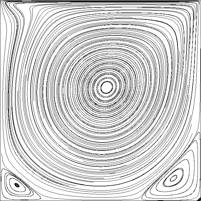
multi mesh

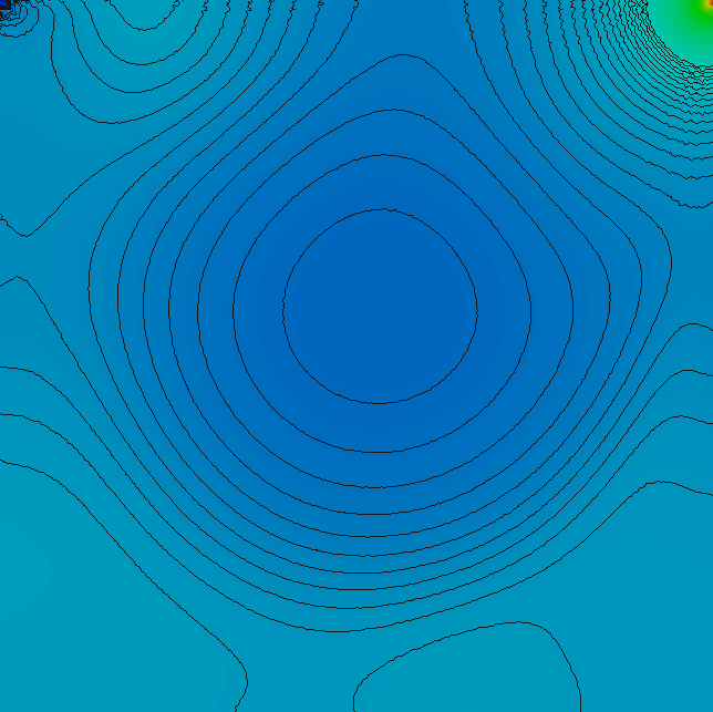
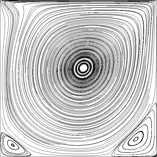
Fig. 8: Results for $Re=1000$. The left column shows 30 pressure isolines in the range $-0.12,0.12$. The right column shows the streamlines contours of the velocity.

	Eddy 1	Eddy 2	Eddy 3	Eddy 4
single-mesh	0.5310,	0.8633,	0.0838,	0.9937,
	0.5658	0.1116	0.0775	0.0062
multi-mesh	0.5305,	0.8669,	0.0813,	0.9953,
	0.5671	0.1125	0.0750	0.0062
Wall	0.5308,	0.8643,	0.0832,	0.9941,
	0.5660	0.1115	0.0775	0.0066
Ghia et al.	0.5313,	0.8594,	0.0859,	0.9922,
	0.5625	0.1094	0.0781	0.0078

Table 2: Comparison of eddy position for $Re=1000$ in the driven cavity model.

In both, the single-mesh method and the multi-mesh method, all finite element spaces have the same number of unknowns. This is the reason, why the usage of the latter one is not faster in contrast to the single-mesh method, as it is the case in dendritic growth. The time for assembling the linear system growth from $4.13$ seconds to $5.79$ seconds, which is mainly caused by the multiplication of the element matrices with the transformation matrices. Instead, the average solution time with a BiCGStab$(\ell)$ solver and ILU preconditioning decreases from $10.18$ seconds to $8.88$ seconds. Although the linear systems have the same number of unknowns, the linear systems resulting from the single-mesh method are denser due to the usage of second order finite elements. The number of non-zero entries decreases around 20% when linear elements are used on both meshes.

5 Conclusion

To further improve efficiency of adaptive finite element simulations we consider the usage of different adaptively refined meshes for different variables in systems of nonlinear, time-depended PDEs. The different variable can have very distinct solution behaviour. To resolve this the meshes can be independently adapted for each variable. Our multi-mesh method works for Lagrange finite elements of arbitrary degree and is independent of the spatial dimension. The approach is well defined, and can be implemented in existing adaptive finite element codes with minimal effort. We have demonstrated for various examples that the resulting linear systems are usually much smaller, when compared to the usage of a single mesh, and the overall computational runtime can be more than halved in various cases. Phase transition problems within a diffuse interface approach are well suited for our approach. The same holds for saddle-point problems in which the inf-sup condition can be fullfilled for finite elements of the same order.

Further examples which are currently under investigation include general diffuse interface concepts to solve PDEs in complex domain. Here a phase-field function is used to describe the domain implicitly [17], which only requires a fine resolution along the boundaries. The approach might also be used in time stepping schemes to prevent loss of information during coarsening. In a classical approach the solution from the old time step is simply interpolated to the new mesh at the new time step. If the new mesh is coarser information is lost, which can be prevented by using the multi-mesh approach for the solution at different time steps. And also in optimal control problems the approach is very promizing, as in many situations the dual solution is much smoother than the primal solution and thus can be discretized on a much coarser mesh using are multi-mesh approach which will be demonstrated for control of an Allen-Cahn equation.

6 Acknowledgement

We would like to thank Rainer Backofen for fruitful discussions. The work has been supported by DFG through Vo899/5-1 and Vo899/11-1.

References

- [1] Simon Vey and Axel Voigt. Amdis: adaptive multidimensional simulations. Comput. Vis. Sci., 10(1):57–67, 2007.
- [2] Alfred Schmidt. A multi-mesh finite element method for phase field simulations. Lecture Notes in Computational Science and Engineering, 32:208–217, 2003.
- [3] Ruo Li. On multi-mesh h-adaptive methods. J. Sci. Comput., 24(3):321–341, 2005.
- [4] Yana Di and Ruo Li. Computation of dendritic growth with level set model using a multi-mesh adaptive finite element method. J. Sci. Comput., 39(3):441–453, 2009.
- [5] Ruo Li Xianliang Hu and Tao Tang. A multi-mesh adaptive finite element approximation to phase field models. Commun. Comput. Phys., 5:1012–1029, 2009.
- [6] L. Dubcova P. Solin, J. Cerveny. Adaptive multi-mesh hp-fem for linear thermoelasticity. Research Report No. 2007-08, The University of Texas at El Paso, 2007.
- [7] Pavel Solin, Lenka Dubcova, and Jaroslav Kruis. Adaptive hp-fem with dynamical meshes for transient heat and moisture transfer problems. J. Comput. Appl. Math., 233(12):3103–3112, 2010.
- [8] W. Joppich and M. Kürschner. MpCCI-a tool for the simulation of coupled applications. Conc. Comput. Prac. Exp., 10:183–192, 2005.
- [9] Rüdger Verfürt. A review of a posteriori error estimation and adaptive mesh-refinement techniques. Teubner, 1996.
- [10] Kunibert G. Siebert Alfred Schmidt. Design of Adaptive Finite Element Software: The Finite Element Toolbox ALBERTA. Springer, 2005.
- [11] R. Verfürth. A posteriori error estimates for nonlinear problems. Finite element discretizations of elliptic equations. Math. Comp., 62(206):445–475, 1994.
- [12] R. Verfürth. A posteriori error estimation and adaptive mesh-refinement techniques. In ICCAM’92: Proceedings of the fifth international conference on Computational and applied mathematics, pages 67–83, Amsterdam, The Netherlands, The Netherlands, 1994. Elsevier Science Publishers B. V.
- [13] Kenneth Eriksson and Claes Johnson. Adaptive finite element methods for parabolic problems i: A linear model problem. SIAM Journal on Numerical Analysis, 28(1):43–77, 1991.
- [14] Willy Dörfler. A convergent adaptive algorithm for poisson’s equation. SIAM J. Numer. Anal., 33(3):1106–1124, 1996.
- [15] Nikolas Provatas and Ken Elder. Phase-field methods in materials science and engineering. Wiley, 2010.
- [16] A. Rätz and A. Voigt. PDEs on surfaces - a diffuse interface approach. Comm. Math. Sci., 4:575–590, 2006.
- [17] X. Li, J. Lowengrub, A. Rätz, and A. Voigt. Solving PDEs in complex geometries. Comm. Math. Sci., 7:81–107, 2009.
- [18] X. Li, J. Lowengrub, A. Rätz, and A. Voigt. Two-phase flow in complex geometries - a diffuse domain approach. Comput. Meth. Eng. Sci., in press.
- [19] K.E. Teigen, A. Rätz, and A. Voigt. A diffuse-interface method for two-phase flows with soluble surfactants. J. Comput. Phys., in review.
- [20] C. Landsberg, F. Stenger, A. Deutsch, M. Gelensky, A. Roesen-Wolff, and A. Voigt. A modeling approach to in situ tissue engineering - chemoattraction of bone marrow stromal cells into three-dimensional biomimetic scaffolds. J. Math. Biol., in review.
- [21] Stefan Turek. Efficient solvers for incompressible flow problems: an algorithmic and computational approach. Springer, 1999.
- [22] W.J. Boettinger, J.A. Warren, C. Beckermann, and A. Karma. Phase-field simulation of solidification. Ann. Rev. Mat. Res., 32, 2002.
- [23] A. Karma and J.W. Rappel. Phase-field method for computationally efficient modeling of solidification with arbitrary interface kinetics. Phys. Rev. E, 53:R3017–R3020, 1996.
- [24] Alain Karma and Wouter-Jan Rappel. Quantitative phase-field modeling of dendritic growth in two and three dimensions. Phys. Rev. E, 57(4):4323–4349, Apr 1998.
- [25] Timothy A. Davis. Algorithm 832: Umfpack v4.3—an unsymmetric-pattern multifrontal method. ACM Trans. Math. Softw., 30(2):196–199, 2004.
- [26] Peter Gottschling, David S. Wise, and Michael D. Adams. Representation-transparent matrix algorithms with scalable performance. In ICS ’07: Proceedings of the 21st annual international conference on Supercomputing, pages 116–125, New York, NY, USA, 2007. ACM.
- [27] M. Bercovier and O. Pironneau. Error estimates for finite element method solution of the Stokes problem in the primitive variables. Numer. Math., 33(2):211–224, 1979.
- [28] R. Verfürth. Error estimates for a mixed finite element approximation of the stokes equations. RAIRO Anal. Numer., 18:175–182, 1984.
- [29] W. A. Wall. Fluid-Struktur-Interaktion mit stabilisierten Finiten Elementen. PhD thesis, Institut für Baustatistik der Universität Stuttgart, 1999.
- [30] U. Ghia, K. N. Ghia, and C. T. Shin. High-re solutions for incompressible flow using the navier-stokes equations and a multigrid method. Journal of Computational Physics, 48(3):387 – 411, 1982.