Limit theorems for a random directed slab graph

Abstract

We consider a stochastic directed graph on the integers whereby a directed edge between $i$ and a larger integer $j$ exists with probability $p_{j-i}$ depending solely on the distance between the two integers. Under broad conditions, we identify a regenerative structure that enables us to prove limit theorems for the maximal path length in a long chunk of the graph. The model is an extension of a special case of graphs studied in [18]. We then consider a similar type of graph but on the ‘slab’ $\mathbb{Z}\times I$, where $I$ is a finite partially ordered set. We extend the techniques introduced in the in the first part of the paper to obtain a central limit theorem for the longest path. When $I$ is linearly ordered, the limiting distribution can be seen to be that of the largest eigenvalue of a $|I|\times|I|$ random matrix in the Gaussian unitary ensemble (GUE).

1 Introduction

Consider a random directed graph with vertex $V=\mathbb{Z}$, the integers. A pair of integers $(i,j)$ is declared to be an edge, directed from $i$ to $j$, with probability $p_{j-i}$ which depends only on the difference $j-i$, and this is done independently from pair to pair. We assume that $p_{k}=0$ for all $k\leq 0$, so there are no directed edges from a larger integer to a smaller one. We are interested in limit theorems (law of large number and central limit theorem) for the maximum length $T[1,n]$ of all paths from 1 to $n$, as $n\to\infty$. The problem as such is related to last-passage percolation.

Unlike nearest-neighbour graphs [28, 3], the quantity $T[1,n]$ does not have a direct subadditive property. It turns out that, a related quantity, namely the maximum $L[1,n]$ of all paths in the restriction of the graph on $\{1,\ldots,n\}$, has an almost sub-additive property (see (2)) and thus $L[1,n]/n\to C$, almost surely, for some deterministic constant $C\leq 1$. It is later shown that any two vertices are almost surely eventually connected by a path, and thus $T[1,n]$ has the same asymptotic properties as $L[1,n]$. The minimal condition we need to carry out our programme is

$$\sum_{k=1}^{\infty}(1-p_{1})\cdots(1-p_{k})<\infty.$$

Under this condition, we can identify a random subset $\SS$ (we call it “skeleton”) of $\mathbb{Z}$ whose points form a stationary renewal process (see Sections 3 and 4) over which the graph regenerates and has the property that any element $v$ of $\SS$ is connected by a path (directed either towards $v$ or away from it) to any other vertex in $\mathbb{Z}$. The quantity $L[1,n]$ becomes additive over the regenerative set $\SS$ enabling us to prove, under the stronger condition

$$\sum_{k=1}^{\infty}k(1-p_{1})\cdots(1-p_{k})<\infty,$$

a (functional) central limit theorem. The latter condition implies finiteness of variance of the longest path between two successive points of $\SS$. To prove the latter assertion, we provide a rather non-trivial algorithmic construction of the last non-positive element of $\SS$. This construction is related to the so-called coupling-from-the past method for perfect simulation [33, 19] and is the topic of Section 6 which is based on the properties of two stopping times studied in Section 5. The central limit theorem is proved in Section 7.

We then consider an extension of the random graph on the vertex set $\mathbb{Z}\times I$, where $I$ is a partially ordered set under some partial order $\preceq$ possessing a minimum and a maximum element. We let an edge from $(x,i)$ to $(y,j)$ exist with probability that depends on $y-x$ and on $i$ and $j$, and only when $y-x>0$ and $i\preceq j$. We let $L_{N}$ be the length of the longest path in the restriction of the graph on $\{0,\ldots,N\}\times i$ and show that the law of $L_{N}$, appropriately normalized, satisfies a functional central limit theorem such that the limit process $(Z_{t},t\geq 0)$ is $1/2$–self-similar, non-Gaussian, continuous process with $Z_{1}$ having the law of the largest eigenvalue of an a $|I|\times|I|$ random matrix in the Gaussian Unitary Ensemble (GUE) [2].

The case where all the $p_{k}$ are equal to $p$ corresponds to a directed version of the classical Erdős-Rényi graph [4]. Indeed, let $G_{n,p}$ be the Erdős-Rényi graph on the set of vertices $\{1,\ldots,n\}$. To each $\{i,j\}$ which is an edge in $G_{n,p}$ we give an orientation from $i\wedge j$ to $i\vee j$. The directed graph thus obtained is precisely the restriction of our graph on the set $\{1,\ldots,n\}$. This model was also studied in [18]. In this paper, we obtained, among other things, sharp estimates for the $C\equiv C(p)$ as a function of $p$. Besides purely mathematical interest, this model is motivated by applications in Mathematical Biology (community food webs) [31, 14, 30], in Computer Science (parallel processing systems) [22], and in Physics. Allowing the connectivity probability to depend on the distance between two vertices $i$ and $j$ means larger modelling flexibility on one hand while making the model more realistic on the other.

In [18] we developed a generalisation of Borovkov’s theory of renovating events [9, 10, 11, 12, 13] in order to construct a Markov chain in infinite dimensions describing the “weights” of vertices. As a matter of fact, in [18], the random graph was a special case of a more general dynamical system (the “infinite bin model”) with stationary and ergodic input. In this paper, we follow a different approach, one that is applicable specifically for cases where there is independence between links. In such a case, the approach has the advantage that it is more elementary using, essentially, renewal theory and coupling between renewal processes.

2 The line model

We are given a set of numbers $(p_{j},j\in\mathbb{N})$, such that

$$0\leq p_{j}<1,\quad j\in\mathbb{N}.$$

and consider $(\alpha_{i,j},~{}i,j\in\mathbb{Z},~{}i<j)$ as a collection of i.i.d. random variables with common law

$$\mathbb{P}(\alpha_{0,1}=1)=1-\mathbb{P}(\alpha_{0,1}=-\infty)=p_{j-i}.$$

Based on this collection, we build a directed random graph $G$ on $\mathbb{Z}$ with edges

$$E=\{(i,j)\in\mathbb{Z}\times\mathbb{Z}:~{}i<j,~{}\alpha_{i,j}=1\}.$$

We shall occasionally refer to the restriction $G[i,j]$ of the graph on the vertex set $\{i,i+1,\ldots,j\}$ (deleting all edges with either of the endpoints not in this set). We are interested in the behaviour of longest paths. A path $\pi$ is an increasing sequence of vertices $\pi=(i_{0},i_{1},\ldots,i_{\ell})$ successively connected by edges, i.e. $\alpha_{i_{0},i_{1}}=\cdots=\alpha_{i_{\ell-1},i_{\ell}}=1$. The number $\ell=|\pi|$ of edges is the length of this path.

For any $\ell\geq 1$ and any increasing sequence $(i_{0},i_{1},\ldots,i_{\ell})$ of vertices we conveniently define

$$|(i_{0},i_{1},\ldots,i_{\ell})|=(\alpha_{i_{0},i_{1}}+\alpha_{i_{1},i_{2}}+\cdots+\alpha_{i_{\ell-1},i_{\ell}})^{+}.$$ (1)

Clearly, this quantity is $0$ if one of the summands takes value $-\infty$; otherwise, it equals $\ell$. In other words, $|(i_{0},i_{1},\ldots,i_{\ell})|>0$ if and only if $(i_{0},i_{1},\ldots,i_{\ell})$ is a path.

We say that there is a path from $i$ to $j$ if $i_{0}=i$, $i_{\ell}=j$; we denote this event by $i\leadsto j$ and may also express it by saying that $i$ leads to $j$ or that $j$ is reachable from $i$.

We let $T[i,j]$ be the maximum length of all paths from $i$ to $j$. Unlike nearest-neighbour directed graph models (see, e.g. [27]), this quantity does not have a subadditivity property. To remedy this we let $L[i,j]$ be the maximum length of all paths from some $i^{\prime}\geq i$ to some $j^{\prime}\leq j$, i.e.,

$$L[i,j]=\max_{i\leq i^{\prime}\leq j^{\prime}\leq j}T[i^{\prime},j^{\prime}].$$

That is, $L[i,j]$ is the longest path of the restricted graph $G[i,j]$. Clearly, $L[i,j]$ has the same law as $L[0,j-i]$. It is also clear that $L[i,j]$ is subadditive in the sense that

$$L[i,k]\leq L[i,j]+L[j,k]+1,\quad i<j<k.$$ (2)

Indeed, if $\pi$ is a path of maximal length in $G[i,k]$ then its restriction $\pi^{\prime}$ on $G[i,j]$ has length at most $L[i,j]$ and its restriction $\pi^{\prime\prime}$ on $G[j,k]$ has length at most $L[j,k]$. Now the length of $\pi$ is equal to the length of $\pi^{\prime}$ plus the length of $\pi^{\prime\prime}$ plus, possibly, 1, if $j$ is not a vertex of $\pi$. By the subadditive ergodic theorem [25, p. 192], there exists a deterministic $C\in[0,1]$ such that

$$\mathbb{P}(\lim_{j\to\infty}L[i,j]/j=C)=1.$$ (3)

Some of the results below do not depend on the independence assumptions between the random variables $\alpha_{i,j}$. It is often necessary to define the model on an appropriate probability space. We do this as follows. Let ${\bm{\delta}}=(\delta_{j},j\in\mathbb{Z})$ be a collection of independent $\{-\infty,1\}$-valued random variables with

$$\mathbb{P}(\delta_{j}=1)=\begin{cases}0,&\text{ if }j\leq 0\\ p_{j},&\text{ if }j>0.\end{cases}$$

Let ${\bm{\delta}}^{(i)}$, $i\in\mathbb{Z}$ be i.i.d. copies of $\bm{\delta}$. The probability space $\Omega$ consists of $\omega=({\bm{\delta}}^{(i)},i\in\mathbb{Z})$. The random variables $\alpha_{i,j}$ are then defined by

$$\alpha_{i,j}(\omega)=\delta^{(i)}_{j-i}.$$

The sigma-field is the standard product sigma-field. A natural shift $\theta$ on $\Omega$ is the map defined by

$$\omega=(i\mapsto{\bm{\delta}}^{(i)})\mapsto\theta\omega=(i\mapsto{\bm{\delta}}^{(i+1)}).$$ (4)

Hence

$$\alpha_{i,j}(\theta\omega)=\delta^{(i+1)}_{j-i}=\delta^{(i+1)}_{(j+1)-(i+1)}=\alpha_{i+1,j+1}(\omega).$$

The random variables $L[i,j]$ are all defined explicitly on $\Omega$ via $L[i,j]=\max_{i\leq i_{0}<i_{1}<\cdots<i_{\ell}\leq j}|(i_{0},\ldots,i_{\ell})|$ where $(i_{0},\ldots,i_{\ell})$ is the random variable defined by (1). It is in this sense that the law $\mathbb{P}$ of the model is $\theta$-invariant on $\Omega$. Moreover, $\theta$ is ergodic. In fact, the result that the asymptotic limit of $L[1,n]/n$ exists depends only on this $\theta$-invariance, so it holds for more general models where the law of ${\bm{\delta}}$ is not that of independent random variables.

A word on notation: If $(A_{n},n\in\mathbb{Z})$ is a collection of events of $\Omega$ and $\tau$ is $\mathbb{Z}$-valued random variable on $\Omega$ then $A_{\tau}$ denotes the event containing all $\omega\in\Omega$ such that $\omega\in A_{\tau(\omega)}$.

3 The skeleton

For the purposes of this section, let $\Omega$ be the space defined above, $\theta$ the natural shift (4), and let $\mathbb{P}$ be a $\theta$-invariant probability measure. In addition, assume that $\theta$ is ergodic, i.e. that the invariant sigma-field is trivial. Recall the shorthand $\{i\leadsto j\}=\{T[i,j]>0\}$ for the event that there is a path from $i$ to $j$. Consider, for each $n\in\mathbb{Z}$, the events

$$A^{+}_{n} :=\bigcap_{j>n}\{n\leadsto j\}=\{\text{any $j>n$ is reachable from $n$}\}$$

$$A^{-}_{n} :=\bigcap_{j<n}\{j\leadsto n\}=\{\text{$n$ is reachable from any $j>n$}\}.$$

The following is an immediate consequence of the definitions:

Lemma 1.

(i) The sequence $\big{(}(A^{-}_{n},A^{+}_{n}),n\in\mathbb{Z}\big{)}$ is stationary and ergodic. (ii) For each $n$, the events $A_{n}^{-}$ and $A_{n}^{+}$ are independent and $\mathbb{P}(A_{n}^{+})=\mathbb{P}(A_{n}^{-})=\mathbb{P}(A_{0}^{+})$.

We are interested in the random set

$$\SS(\omega):=\{n\in\mathbb{Z}:~{}\omega\in A_{n}^{+}\cap A_{n}^{-}\},$$ (5)

and refer to it as the skeleton of the random graph. The terminology is supposed to be reminiscent of a point of view described next.

Let $\mathscr{P}(E)\subset\mathbb{Z}\times\mathbb{Z}$ be a partial order (i.e. if $(i,j),(j,k)\in\mathscr{P}(E)$ then $(i,k)\in\mathscr{P}(E)$) which contains the set of edges $E$. In fact, take $\mathscr{P}(E)$ to be the smallest such set. Necessarily, $\mathscr{P}(E)=\{(i,j)\in\mathbb{Z}\times\mathbb{Z}:~{}i\leadsto j\}$. A subset $U$ of $\mathbb{Z}$ is totally ordered under the partial order $\leadsto$ if for any distinct $i,j\in U$ we either have $i\leadsto j$ or $j\leadsto i$. We say that a totally ordered subset $U$ is special if it has the stronger property that for all distinct $i,j$ with $i\in U$ and $j\in V$, we either have $i\leadsto j$ or $j\leadsto i$. Clearly, the union of special totally ordered subsets is special; thus we can speak of the maximal special totally ordered subset and we refer to it as the skeleton of the partial order. Adopting this definition, it is now clear that the set $\SS$ defined by (5) is the skeleton of the partial order $\leadsto$ on $\mathbb{Z}$. In [1] the elements of $\SS$ are referred to as posts. In fact, [1] uses $\SS$ in order to derive limit theorems of the number $N_{n}$ of linear extensions of the the random partial order $\leadsto$ on $\{1,\ldots,n\}$.

For a general partially ordered set, a skeleton may not exist. However, in our case, the condition $\mathbb{P}(A_{0}^{+}\cap A_{0}^{-})>0$ is sufficient for $\SS$ to be almost surely infinite.

Lemma 2.

If $\lambda:=\mathbb{P}(A_{0}^{+}\cap A_{0}-)>0$ then $\SS$ is an a.s. infinite set.

Proof.

Let $\theta$ be the shift defined by (4). Then, for all $\omega$, $\SS(\omega)=\SS(\theta\omega)$. Since $\mathbb{P}$ is $\theta$-invariant, the result follows. ∎

Assuming that $\lambda=\mathbb{P}(A_{0}^{+}\cap A_{0}^{-})>0$, we may then, equivalently, consider $\SS$ as a stationary-ergodic point process on the integers with rate $\lambda$ because $\lambda=\mathbb{P}(0\in\SS)$. We let $\Gamma_{n}$, $n\in\mathbb{Z}$ be an enumeration of the elements of $\SS$ according to the following convention:

$$\cdots<\Gamma_{-1}<\Gamma_{0}\leq 0<\Gamma_{1}<\Gamma_{2}<\cdots\$$

In particular, $\Gamma_{0}$ is the largest non-negative element of $\SS$.

We can now strengthen the subadditivity property (2) for $L$:

Lemma 3.

For all integers $m<n$,

$$L{[\Gamma_{m},\Gamma_{n}]}=L{[\Gamma_{m},\Gamma_{m+1}]}+\cdots+L{[\Gamma_{n-1},\Gamma_{n}]}.$$

Proof.

To see this, consider the interval $[\Gamma_{1},\Gamma_{n}]$ and a path $\pi^{*}$ of length $L{[\Gamma_{1},\Gamma_{n}]}$. Then this path must visit all the intermediate skeleton points $\Gamma_{1},\ldots,\Gamma_{n}$. Indeed, suppose this is not the case and $\pi^{*}$ does not visit, say, $\Gamma_{l}$, for some $1\leq l\leq n$. Consider an edge $(i,j)$ belonging to $\pi^{*}$, with $i\leq\Gamma_{l}\leq j$. By the definition of $\Gamma_{l}$, both $(i,\Gamma_{l})$ and $(\Gamma_{l},j)$ are edges of the random graph $G$. Therefore we can increase the length of $\pi^{*}$ by $1$ if we replace the edge $(i,j)$ by two edges $(i,\Gamma_{l})$ and $(\Gamma_{l},j)$. This leads to the contradiction since $\pi^{*}$ has length $L{[\Gamma_{1},\Gamma_{n}]}$ which is, by definition, maximal. ∎

4 Regenerative structure

Throughout, we make use of the following two conditions:
          [C1]   $\displaystyle 0<p_{1}<1$ [C2]   $\displaystyle\sum_{k=1}^{\infty}(1-p_{1})\cdots(1-p_{k})<\infty$.
We also sometimes write $q_{j}=1-p_{j}$. For each $j\in\mathbb{Z}$ we consider its immediate neighbours:

$$\overline{\eta}(j) :=\min\{k>j:~{}\alpha_{j,k}=1\}$$

$$\overline{\xi}(j) :=\max\{i<j:~{}\alpha_{i,j}=1\}.$$ (6)

See Figure 1. The distances of these vertices from $j$ are denoted as follows:

$$\eta(j) :=\overline{\eta}(j)-j$$

$$\xi(j) :=j-\overline{\xi}(j).$$

Notice that $(\xi(j),j\in\mathbb{Z})$ and $(\eta(j),j\in\mathbb{Z})$ are identically distributed sequences, and that each one is a sequence of i.i.d. random variables. Furthermore, for each $j\in\mathbb{Z}$,

$$(\xi(j+1),\xi(j+2),\ldots)\perp\!\!\!\perp(\eta(j-1),\eta(j-2),\ldots)$$

Henceforth, we shall let $\xi$ be a random variable with distribution the common distribution of $\xi(j)$ and $\eta(j)$:

$$\mathbb{P}(\xi>n)=\mathbb{P}(\xi(0)>n)=\mathbb{P}(\eta(0)>n)=(1-p_{1})\cdots(1-p_{n}),\quad n\in\mathbb{N}.$$

Figure 1: Notation used: $\overline{\xi}(j)$ is the first vertex below $j$ that is connected to $j$; correspondingly, $\overline{\eta}(j)$ is the first vertex above $j$ connected to $j$.

Define next the events

$$A_{u,v}^{+}:=\bigcap_{j=u+1}^{v}\{u\leadsto j\},\quad A_{u,v}^{-}:=\bigcap_{j=u}^{v-1}\{j\leadsto v\},$$ (7)

for which, clearly,

$$A^{+}_{u,v}\supset A^{+}_{u,v+1},\quad A^{-}_{u,v}\supset A^{-}_{u-1,v}$$

with

$$\lim_{v\to\infty}A_{u,v}^{+}=A_{u}^{+},\quad\lim_{u\to-\infty}A_{u,v}^{-}=A_{v}^{-}.$$ (8)

Furthermore,

$$A_{u,v}^{+}\cap A_{v,w}^{+}\subset A_{u,w}^{+},\text{ if }u<v<w,$$ (9)

a property we shall use in Section 6. Observe also the following:

Lemma 4.

For all integers $u<v$,

$$A_{u,v}^{+} =\bigcap_{j=u+1}^{v}\bigcup_{i=u}^{j-1}\{i\leadsto j\}=\bigcap_{j=u+1}^{v}\{u\leq\overline{\xi}(j)\}$$

$$A_{u,v}^{-} =\bigcap_{j=u}^{v-1}\bigcup_{i=j+1}^{v}\{j\leadsto i\}=\bigcap_{j=u}^{v-1}\{\overline{\eta}(j)\leq v\}$$

$$A_{u}^{+} =\bigcap_{j>u}~{}\bigcup_{i=u}^{j-1}\{i\leadsto j\}=\bigcap_{j>u}\{u\leq\overline{\xi}(j)\}$$

$$A_{v}^{-} =\bigcap_{j<v}~{}\bigcup_{i=j+1}^{v}\{j\leadsto i\}=\bigcap_{j<v}\{\overline{\eta}(j)\leq v\}.$$

Proof.

We prove the first equality. That $A_{u,v}^{+}\subset\cap_{j=u+1}^{v}\cup_{i=u}^{j-1}\{i\leadsto j\}$ is immediate from the definition (7). To prove the opposite inclusion, assume that $u>v+1$ (otherwise there is nothing to prove) and that for all integers $j\in[u+1,v]$ there exists an integer $i\in[u,j-1]$ such that $i\leadsto j$. Fix $j>u$ and pick $i_{1}$ to be the largest among the vertices between $u$ and $j-1$ such that $i_{1}\leadsto j$; necessarily, $\alpha_{i_{1},j}=1$. Then pick the largest vertex $i_{2}$ among the vertices between $u$ and $i_{1}-1$ such that $i_{2}\leadsto i_{1}$, and continue this way. Since $i_{1}>i_{2}>\cdots\geq u$, it follows that this process terminates with some $i_{k}=u$. Since $(u=i_{k},i_{k+1},\ldots,i_{1},j)$ is a path, we have that $u\leadsto j$. The second equality for $A_{u,v}^{+}$ now follows from the definition (6). The relations for $A_{u,v}^{-}$ follow similarly. The third (respectively, fourth) line is obtained by sending $v$ to $+\infty$ (respectively, $u$ to $-\infty$) in the first (respectively, second) one. ∎

This lemma tells us that $A_{u,v}^{+}$ is the intersection of $v-u$ independent events. Indeed, since $\overline{\xi}(j)=j-\xi(j)$ we have

$$A_{u,v}^{+}=\{\xi(u+1)\leq 1,\xi(u+2)\leq 2,\ldots,\xi(v)\leq v-u\},$$ (10)

and the random variables $\xi(u+1),\ldots,\xi(v)$ are i.i.d. Similarly, for $A_{u,v}^{-}$,

$$A_{u,v}^{-}=\{\eta(u)\leq v-u,\ldots,\eta(v-2)\leq 2,\eta(v-1)\leq 1\}.$$ (11)

Moreover, since

$$(\xi(u+1),\xi(u+2),\ldots,\xi(v))\stackrel{{\scriptstyle\text{d}}}{{=}}(\eta(v-1),\eta(v-2),\ldots,\eta(u))$$

we have that $\mathbb{P}(A_{u,v}^{+})=\mathbb{P}(A_{u,v}^{-})$. Similarly, both $A_{n}^{+}$ and $A_{n}^{-}$ are intersections of infinitely many independent events:

$$A_{n}^{+} =\bigcap_{j>n}\{\xi(j)\leq j-n\}$$ (12)

$$A_{n}^{-} =\bigcap_{j<n}\{\eta(j)\leq n-j\},$$ (13)

and $\mathbb{P}(A_{n}^{+})=\mathbb{P}(A_{n}^{-})$. The skeleton (5) can be expressed as follows:

$$\SS=\{n\in\mathbb{Z}:~{}\sup_{i<n}\overline{\eta}(i)\leq n\leq\inf_{j>n}\overline{\xi}(j)\}.$$ (14)

Regarding $\SS$ as a point process, we see that it has rate

$$\lambda=\mathbb{P}(0\in\SS)=\mathbb{P}(A_{0}^{+})^{2}=\big{(}\prod_{j=1}^{\infty}\mathbb{P}(\xi(j)\leq j)\big{)}^{2}=\prod_{j=1}^{\infty}[1-\mathbb{P}(\xi(0)>j)]^{2}.$$

Since

$$\mathbb{P}(\xi(0)>j)=\mathbb{P}(\alpha_{0,1}=\cdots=\alpha_{0,j}=0)=(1-p_{1})\cdots(1-p_{j}),$$ (15)

we have

$$\lambda=\prod_{j=1}^{\infty}[1-(1-p_{1})\cdots(1-p_{j})]^{2}$$ (16)

and so

$$\text{{\sf[C2]} }\iff\lambda>0\iff\mathbb{E}[\xi(0)]<\infty.$$

Consider now two successive skeleton points $\Gamma_{k}$ and $\Gamma_{k+1}$ and let $\mathscr{C}_{k}(\omega)$ be the restriction of $\omega$ on $[\Gamma_{k},\Gamma_{k+1})$:

$$\mathscr{C}_{k}:=\big{(}\bm{\delta}^{(n)},~{}\Gamma_{k}\leq n<\Gamma_{k+1}\big{)},\quad k\in\mathbb{Z};$$

we refer to it as the $k$-th “cycle”. We next show that the sequence of cycles have a regenerative structure in the following sense:

Lemma 5.

The cycles $(\mathscr{C}_{k},k\in\mathbb{Z})$ are independent and $(\mathscr{C}_{k},k\in\mathbb{Z}-\{0\})$ are identically distributed. In particular, the skeleton vertices $(\Gamma_{k},k\in\mathbb{Z})$ form a stationary renewal process.

Intuitively, Lemma 5 is based on the following observation. Suppose that $0$ is a skeleton vertex (i.e. condition on the event $A_{0}^{-}\cap A_{0}^{+}$). Then $\overline{\xi}(1)\geq 0$, $\overline{\xi}(2)\geq 0$, etc. In other words, $\overline{\xi}(1)=0$, $\overline{\xi}(2)\in\{1,2\}$, $\overline{\xi}(3)\in\{0,1,2\}$, etc. To determine the location of the next skeleton vertex after $0$ we need to find the first vertex $j>0$ such which is connected with every vertex between $0$ and $j-1$. This means that, conditional on $0$ being a skeleton vertex, the location of the first skeleton vertex larger than $0$ does not depend on the $(\bm{\delta}^{(n)},n<0)$.

Proof of Lemma 5.
For $k\geq 1$, let $\mathscr{F}_{k}^{+}$ be the sigma-algebra generated by $(\bm{\delta}^{(1)},\ldots,\bm{\delta}^{(k)})$ and let $\mathscr{F}_{k}^{-}$ be the sigma-algebra generated by $(\bm{\delta}^{(-1)},\ldots,\bm{\delta}^{(-k)})$. It suffices to prove that, for any $k\geq-1$, $l\geq 1$, and any $B_{k}^{-}\in\mathscr{F}_{k}^{-}$, $B_{l}^{+}\in\mathscr{F}_{l}^{+}$,

$$\mathbb{P}(\Gamma_{-1}=k,B^{-}_{k},\Gamma_{1}=l,B^{+}_{l}\mid\Gamma_{0}=0)=\mathbb{P}(\Gamma_{-1}=k,B^{-}_{k}\mid\Gamma_{0}=0)\mathbb{P}(\Gamma_{1}=l,B^{+}_{l}\mid\Gamma_{0}=0).$$

Assume that $\Gamma_{0}=0$ (i.e. $0$ is a skeleton vertex). Then, by (14),

$$\ldots,~{}\overline{\eta}(-2),~{}\overline{\eta}(-1)\leq 0\leq\overline{\xi}(1),~{}\overline{\xi}(2),~{}\ldots$$

In view of the latter inequality, we have

$$\Gamma_{-1} =\max\{n<0:~{}{\text{\Large$\mathfrak{1}$}}_{A_{n}^{-}\cap A_{n}^{+}}=1\}$$

$$=\max\{n<0:~{}\ldots,~{}\overline{\eta}(n-2),~{}\overline{\eta}(n-1)\leq n\leq\overline{\xi}(n+1),~{}\overline{\xi}(n+2),~{}\ldots\}$$

$$=\max\{n<0:~{}\ldots,~{}\overline{\eta}(n-2),~{}\overline{\eta}(n-1)\leq n\leq\overline{\xi}(n+1),~{}\overline{\xi}(n+2),~{}\ldots,~{}\overline{\xi}(0)\}=:\widehat{\Gamma}_{-1},$$

where the last serves as a definition of a new random variable $\widehat{\Gamma}_{-1}$. This random variable is $\mathscr{F}^{-}$-measurable, where $\mathscr{F}^{-}$ is the sigma-algebra generated by $(\bm{\delta}^{(k)},k<0)$. Similarly, we define

$$\widehat{\Gamma}_{1}:=\min\{n>0:~{}\overline{\eta}(0),\ldots,\overline{\eta}(n-1)\leq n\leq\overline{\xi}(n+1),\overline{\xi}(n+2),\ldots\},$$

a random variable which is $\mathscr{F}^{+}$-measurable, where $\mathscr{F}^{+}$ is the sigma-algebra generated by $(\bm{\delta}^{(k)},k>0)$, and observe that, on $\{\Gamma_{0}=0\}$, the random variables $\Gamma_{1}$ and $\widehat{\Gamma}_{1}$ coincide. Note that $\mathscr{F}^{-}$ and $\mathscr{F}^{+}$ are independent. Hence, for $k\leq-1$, $\ell\geq 1$, we have

$$\mathbb{P}(\Gamma_{-1}=k,B^{-}_{k},\Gamma_{1}=l,B^{+}_{l} |\Gamma_{0}=0)$$

$$=\frac{\mathbb{P}(\Gamma_{-1}=k,B^{-}_{k},\Gamma_{1}=l,B^{+}_{l},A_{0}^{+}\cap A_{0}^{-})}{\mathbb{P}(A_{0}^{+}\cap A_{0}^{-})}$$

$$=\frac{\mathbb{P}(\{\widehat{\Gamma}_{-1}=k\}\cap A_{0}^{-}\cap B^{-}_{k},\{\widehat{\Gamma}_{1}=l\}\cap A_{0}^{+}\cap B^{+}_{l})}{\mathbb{P}(A_{0}^{+})\mathbb{P}(A_{0}^{-})}$$

$$=\frac{\mathbb{P}(\{\widehat{\Gamma}_{-1}=k\}\cap A_{0}^{-}\cap B^{-}_{k})~{}\mathbb{P}(\{\widehat{\Gamma}_{1}=l\}\cap A_{0}^{+}\cap B^{+}_{l})}{\mathbb{P}(A_{0}^{+})\mathbb{P}(A_{0}^{-})}$$

$$=\mathbb{P}(\widehat{\Gamma}_{-1}=k,B^{-}_{k}\ |\ A_{0}^{-})~{}\mathbb{P}(\widehat{\Gamma}_{1}=l,B^{+}_{l}\ |\ A_{0}^{+}).$$

Note that

$$\mathbb{P}(\widehat{\Gamma}_{-1}=k,B^{-}_{k}\ |\ A_{0}^{-})=\mathbb{P}(\widehat{\Gamma}_{-1}=k,B^{-}_{k}\ |\ A_{0}^{-}\cap A_{0}^{+})\\ =\mathbb{P}(\Gamma_{-1}=k,B^{-}_{k}\ |\ A_{0}^{-}\cap A_{0}^{+})=\mathbb{P}(\Gamma_{-1}=k,B^{-}_{k}\ |\Gamma_{0}=0).$$

Similarly,

$$\mathbb{P}\{\widehat{\Gamma}_{1}=1,B^{+}_{l}\ |\ A_{0}^{+}\}=\mathbb{P}\{\Gamma_{1}=1,B^{+}_{l}\ |\Gamma_{0}=0\}.$$

∎

Corollary 1.

The bivariate random variables

$$\big{(}\Gamma_{1}-\Gamma_{0},~{}L[\Gamma_{0},\Gamma_{1}]\big{)},~{}~{}\big{(}\Gamma_{2}-\Gamma_{1},~{}L[\Gamma_{1},\Gamma_{2}]\big{)},~{}~{}\ldots$$

are i.i.d.

5 Two stopping times

In this section, we study properties of the following two random variables:

$$\mu :=\inf\{i>0:~{}{\text{\Large$\mathfrak{1}$}}_{A_{-i,0}^{-}}=0\}$$

$$\nu :=\inf\{i>0:~{}{\text{\Large$\mathfrak{1}$}}_{A_{-i,0}^{+}}=1\}.$$

These random variables are important in the algorithmic construction of Section 6.

Note that $-\nu$ is the first vertex $<0$ with the property that every vertex in the interval $(-\nu,0]$ is reachable from $-\nu$:

$$\nu=\inf\{i>0:~{}-\nu\leadsto 0,~{}-\nu\leadsto-1,~{}\ldots,~{}-\nu\leadsto-\nu+1\}.$$

Also, $-\mu$ is the first vertex $<0$ such that $0$ is not reachable from $-\mu$:

$$\mu=\inf\{i>0:~{}-i\not\leadsto 0\}.$$

We will show that $\mu$ is a defective random variable, i.e. that $\mathbb{P}(\mu=\infty)>0$, with conditional tail $\mathbb{P}(\mu>n|\mu<\infty)$ comparable to the integrated tail of $\xi$. We will also show that $\nu$ is an a.s. finite random variable with the same number of moments as $\xi$.

Note first that both $\mu$ and $\nu$ are stopping times with respect to the filtration $(\mathscr{F}_{k}^{-},k\leq 0)$. Observe that

$$\{\mu=\infty\}=\bigcap_{i\geq 1}A_{-i,0}^{-}=A_{0}^{-}.$$ (17)

Since condition [C2] is equivalent to $\mathbb{P}(A_{0}^{-})>0$, we have

$$\mathbb{P}(\mu=\infty)>0.$$

On the other hand,

$$\{\nu=\infty\}=\bigcap_{n=1}^{\infty}(A_{-n,0}^{+})^{c},$$

and, as we shall see below, this event has probability zero:

$$\mathbb{P}(\nu=\infty)=0.$$ (18)

Let us first focus on the law of $\mu$, conditional on $\{\mu<\infty\}$. This can be computed easily, from the definition of $\mu$, and equations (11), (17), and (15).

$$\mathbb{P}(n<\mu<\infty) =\mathbb{P}(\eta(-k)\leq k\text{ for all }1\leq k\leq n)~{}\mathbb{P}(\eta(-m)>m\text{ for some }m>n)$$ (19)

$$=\prod_{k=1}^{n}\mathbb{P}(\eta(-k)\leq k)~{}\bigg{(}1-\prod_{m=n+1}^{\infty}\mathbb{P}(\eta(-m)\leq m)\bigg{)}$$

$$=(1-q_{1})(1-q_{1}q_{2})\cdots(1-q_{1}q_{2}\cdots q_{n})\bigg{(}1-\prod_{m=n+1}^{\infty}(1-q_{1}q_{2}\cdots q_{m})\bigg{)}$$

Conditional on $\{\mu<\infty\}$, the random variable $\mu$ has a tail comparable to the integrated tail of $\xi$:

Lemma 6.

Suppose that [C1] and [C2] hold. There exist constants $0<C_{1}<C_{2}<\infty$ such that, for all $n\geq 0$,

$$C_{1}\sum_{m>n}^{\infty}\mathbb{P}(\xi>m)\leq\mathbb{P}(\mu>n\ |\ \mu<\infty)\leq C_{2}\sum_{m>n}^{\infty}\mathbb{P}(\xi>m).$$

Proof.

Since $p_{1}<1$, we have $\lambda<1$ (see (16)) and so

$$\mathbb{P}(\mu<\infty)=1-\lambda^{1/2}>0.$$

Using (19) we have

$$\mathbb{P}(\mu>n\ |\ \mu<\infty) \leq\frac{1}{1-\lambda^{1/2}}~{}\sum_{m=n+1}^{\infty}\mathbb{P}(\eta(m)>m)=\frac{1}{1-\lambda^{1/2}}~{}\sum_{m=n+1}^{\infty}\mathbb{P}(\xi>m).$$

Hence $C_{1}=1/(1-\lambda^{1/2})$. To obtain a bound from below note that the first term on the right of $\eqref{muexact}$ is $\geq\mathbb{P}(\mu=\infty)$ and so

$$\mathbb{P}(n<\mu<\infty) =\lambda^{1/2}\bigg{(}1-\prod_{m=n+1}^{\infty}\mathbb{P}(\eta(-m)\leq m)\bigg{)}$$

$$\geq\lambda^{1/2}\bigg{(}1-\exp\big{(}-\sum_{m=n+1}^{\infty}\mathbb{P}(\xi>m)\big{)}\bigg{)}$$

$$\geq\lambda^{1/2}g(\mathbb{E}\xi)\sum_{m=n+1}^{\infty}\mathbb{P}(\xi>m),$$

where $g(x)=(1-e^{-x})/x$. Hence $C_{2}=g(\mathbb{E}\xi)\lambda^{1/2}/(1-\lambda^{1/2}))$. ∎

We next prove something stronger than (18), namely that $\nu$ has the same number of moments as $\xi$.

Lemma 7.

If $\mathbb{E}\xi^{r}<\infty$ for some $r\geq 1$ then $\mathbb{E}\nu^{r}<\infty$.

Proof.

By the definition of $\nu$ and equation (10) we have

$$\nu=\inf\{n\geq 1:~{}\xi(0)\leq n,\xi(-1)\leq n-1,\ldots,\xi(-(n-1))\leq 1\}$$

Define a sequence of non-negative random variables $x_{0},x_{1},x_{2},\ldots$ by $x_{0}=0$ and

$$x_{n}=\max\{\xi(0)-n,\xi(-1)-(n-1),\ldots,\xi(-(n-1))-1\},\quad n\geq 1.$$

Then

$$\nu=\inf\{n\geq 1:~{}x_{n}=0\}.$$

The $x_{n}$ satisfy

$$x_{n+1}=\max(x_{n},\xi(-n))-1,\quad n\geq 0,$$

and, since the $\xi(-n)$ are i.i.d., $(x_{n},n\geq 0)$ is a Markov chain in $\mathbb{Z}_{+}$. We now make two observations that imply the statement of the lemma. First, if $x_{n}>K>0$ then

$$x_{n+1}-x_{n}=(\xi(-n)-x_{n})^{+}-1\leq(\xi(-n)-K)^{+}-1.$$

But $\mathbb{E}[(\xi-K)^{+}]<1$ for sufficiently large $K$. Therefore, after the Markov chain leaves the interval $[0,K]$ (for sufficiently large $K$) it is majorized from above by a random walk with increments distributed like $(\xi-K)^{+}-1$ whose mean is negative. By standard properties of random walks this implies that the return time $T_{K}$ to the set $[0,K]$ satisfies $\mathbb{E}T_{K}^{r}<\infty$ if $\mathbb{E}((\xi-K)^{+}-1)^{r}<\infty$; and the latter is equivalent to $\mathbb{E}\xi^{r}<\infty$. The second observation is that the Markov chain $(x_{n})$ returning to the set $[0,K]$ eventually hits point $0$ after a geometric number of trials. ∎

Corollary 2.

If [C2] holds then $\mathbb{E}\nu<\infty$.

6 Algorithmic construction of $\Gamma_{0}$

In this section we give a method for constructing a specific skeleton point, e.g., the first one which is to the left of the origin. This is the point $\Gamma_{0}$. Besides the theoretical interest, such a construction will be used later for proving a central limit theorem; it can also be used in connection to a perfect simulation algorithm for estimating the value of $C=\lim_{n\to\infty}L[1,n]/n$ (see remarks at the end of the section).

The idea for the construction of $\Gamma_{0}$ is this: recall that $-\nu$ which is the first vertex $<0$ which is connected to every point between $-\nu$ and $0$. We check whether $-\nu$ is also reachable from every point from the left. If it is, we declare that $-\nu$ is a silver point and stop the procedure. If not, there is a first vertex before $-\nu$ which fails to be connected to $-\nu$. Using the shift operator $\theta$ defined in (4), this vertex is at distance $\mu\raisebox{0.43057pt}{\scriptsize$\circ$}\theta^{-\nu}$ from $-\nu$; in other words, this distance is the functional $\mu$ applied to the shifted $\omega$, when the origin is placed at $-\nu$. We then set $\mu[1]=\nu+\mu\raisebox{0.43057pt}{\scriptsize$\circ$}\theta^{-\nu}$, which is the location of the previous vertex, and $\nu[1]=\nu$ and this finishes the first step of the procedure.

The second step of the algorithm is similar to the first one: we search for the first vertex $-\nu[2]$ before $-\mu[1]$ which is connected to every vertex between $-\nu[2]$ and $-\nu[1]$. We know that we can find such a vertex with probability one. If it also happens that $-\nu[2]$ is reachable from any point from the left, we stop and declare $-\nu[2]$ as our silver point. Otherwise, there will be a first vertex, $-\mu[2]<-\nu[2]$ which fails to be connected to $-\nu[2]$.

The procedure continues in the same way, until the first silver point is found, and it will be found with probability one. This first silver point will have the property that it is reachable from every point from the left and is connected to every point up until the origin; see Lemma 10 below. The distribution of this first silver point is well-understood and this is the content of Lemma 9. In fact, we will show that there are infinitely many silver points which form a (delayed) renewal process backwards; see Lemma 12. Finally, in Theorem 1 we show that among the infinitude of silver points we can pick a gold one, namely the point $\Gamma_{0}$.

To define the algorithm explicitly, we consider a sequence of $\mathbb{N}\cup\{+\infty\}$-valued stopping times relative to the filtration $(\mathscr{F}_{k},k\geq 1)$, defined as follows. Let

$$\nu[1] :=\nu$$

$$\mu[1] :=\nu+\mu\raisebox{0.43057pt}{\scriptsize$\circ$}\theta^{-\nu}=\inf\{j>\nu:~{}{\text{\Large$\mathfrak{1}$}}_{A^{-}_{-j,-\nu}}=0\},$$ (20)

and, recursively, for $k\geq 2$,

$$\nu[k] :=\inf\{j>\mu[k-1]:{\text{\Large$\mathfrak{1}$}}_{A_{-j,-\nu[k-1]}^{+}}=1\}$$

$$\mu[k] :=\nu[k]+\mu\raisebox{0.43057pt}{\scriptsize$\circ$}\theta^{-\nu[k]}=\inf\{j>\nu[k]:{\text{\Large$\mathfrak{1}$}}_{A_{-j,-\nu[k]}^{-}}=0\},$$ (21)

where $\theta$ is the natural shift (4). It is understood that if for some $k$ we have $\mu[k]=\infty$ then $\nu[j]=\mu[j]=\infty$ for all $j\geq k+1$. We thus obtain an increasing sequence of stopping times

$$\nu=\nu[1]<\mu[1]<\nu[2]<\mu[2]<\nu[3]<\mu[3]<\cdots$$

which (since $\mathbb{P}(\mu=\infty)>0$) is eventually equal to infinity. It is convenient to think of these stopping times as the points of an alternating point process (the $\mu$-points and the $\nu$-points). In words, the sequence of these stopping times is defined by first laying a $\nu$-point in location $\nu[1]$. Then, as long as $\eta(-(\nu[1]+i))\leq i$ for $i=1,2,\ldots$, we place no point in location $\nu[1]+i$. At the first instance $i$ at which $\eta(-(\nu[1]+i))>i$, we place a $\mu$-point in location $\nu[1]+i$ and call it $\mu[1]$. The random variables $(\eta(-(\nu[1]+i)),i\geq 1)$ are independent of $\nu[1]$, and so the event that we place a $\mu$-point in a finite location is independent of $\nu[1]$ and has probability $\mathbb{P}(\mu<\infty)=1-\lambda^{1/2}$. The procedure continues in the same way: having placed $\nu[k]<\infty$, we decide, independently of the past (i.e. $\mathscr{F}_{\nu[k]}^{-}$) whether to create a new $\mu$-point or not (i.e. place it at infinity). If we do create a new $\mu$-point $\mu[k]$ then, clearly, $\nu[k+1]$ is also finite and $\nu[k+1]-\nu[k]$ has the same distribution as $\nu[2]-\nu[1]$ conditional on $\mu[1]<\infty$. Thus for each $\omega$, the recursion stops at the index

$$K:=\inf\{k\geq 1:~{}\mu[k]=\infty\}.$$ (22)

From the discussion above we immediately obtain:

Lemma 8.

Assume that [C1] and [C2] hold. Then $K$ is a geometric random variable with

$$\mathbb{P}(K>k)=(1-\lambda^{1/2})^{k},\quad k\geq 0.$$

By definition, $\mu[K]=\infty$ but $\mu[K-1]<\infty$. Hence

$$\nu[K]<\infty,\text{ a.s.}$$

Note 1.

We stop for a minute to point out that the whole purpose of the construction of these random variables is the random variable $\nu[K]$. In other words, for each $\omega\in\Omega$, we apply recursion (20)-(21) to obtain the alternating sequence of $\nu$ and $\mu$- points, through them we define that index $K$ as in (22) and, finally, $\nu[K]$. Thus, $\nu[K]$ is a well-defined (measurable) function of $\omega$. We refer to $-\nu[K]$ as the first silver point before $0$.

Although $K$ depends on the whole alternating process $(\nu[k],\mu[k]),k\geq 1)$, we can identify the law of $\nu[K]$ as follows:

Lemma 9.

On a new probability space, let $K,\psi_{1},\psi_{2},\psi_{3},\ldots$ be independent random variables with distributions

$$P(K>k)=(1-\lambda^{1/2})^{k},\quad k\geq 0$$

$$\psi_{1}\stackrel{{\scriptstyle\text{d}}}{{=}}\nu$$

$$\psi_{i}\stackrel{{\scriptstyle\text{d}}}{{=}}\big{(}\nu[2]-\nu[1]\mid\mu[1]<\infty)\stackrel{{\scriptstyle\text{d}}}{{=}}\big{(}\inf\{j>\mu:~{}{\text{\Large$\mathfrak{1}$}}_{A_{-j,0}^{+}}=1\}\mid\mu<\infty\big{)},\quad i\geq 2.$$

Then, assuming [C1] and [C2],

$$\nu[K]\stackrel{{\scriptstyle\text{d}}}{{=}}\psi_{1}+\sum_{i=1}^{K-1}\psi_{i+1}.$$ (23)

Proof.

It follows from

$$\nu[K]=\nu[1]+\sum_{i=1}^{K-1}(\nu[i+1]-\nu[i]).$$

using a simple probabilistic argument as described above. ∎

The reason we are interested in the random variable $\nu[K]$ is the following:

Lemma 10.

Assume [C1] and [C2] hold. Then for $\mathbb{P}$-a.e. $\omega$

$$\omega\in A_{-\nu[K]}^{-}\cap A_{-\nu[K],0}^{+}.$$ (24)

Note that replacing the index $n$ in a sequence of events $A_{n}$ by a random index $N$ amounts to defining the event $A_{N}=\{\omega\in\Omega:\text{ there exists }n\text{ such that }n=N(\omega)\text{ and }\omega\in A_{n}\}$.

The meaning of (24) is that the vertex $\nu[K]$ of the random graph has the property that there is a path from every $j<\nu[K]$ to $\nu[K]$ and there is a path from $\nu[K]$ to every $i$ such that $\nu[K]<i\leq 0$. Our goal is to identify a skeleton point. Whereas $\nu[K]$ is not a skeleton point for sure, there is a positive probability that it is.

Proof of Lemma 10. If $K=k$, for some $k\geq 1$, then $\mu[k]=\infty$ but $\mu[k-1]<\infty$, so $\nu[k]<\infty$ and ${\text{\Large$\mathfrak{1}$}}_{A_{-j,-\nu[k]}^{-}}=0$ for all $j>\nu[k]$. Hence

$$\{K=k\}\subset\bigcap_{j>\nu[k]}A_{-j,-\nu[k]}^{-}=A_{-\nu[k]}^{-},$$

by (8). Also, if $K=k$, then $\nu[k],\nu[k-1],\ldots,\nu[1]<\infty$ and so

$$\{K=k\}\subset A^{+}_{-\nu[k],-\nu[k-1]}\cap A^{+}_{-\nu[k-1],-\nu[k-2]}\cap\cdots\cap A^{+}_{-\nu[1],0}\subset A^{+}_{-\nu[k],0},$$

by (9). But $K$ is a geometric random variable and hence $K<\infty$, a.s. ∎

We also have the following result concerning moments of $\nu[K]$:

Lemma 11.

Assume [C1] and [C2] hold. If, in addition, there exists $r\geq 1$ such that $\mathbb{E}\xi^{r+1}<\infty$, then $\mathbb{E}\nu[K]^{r}<\infty$.

Proof.

We have that $\mathbb{E}\nu[K]^{r}<\infty$ if $\mathbb{E}\nu^{r}<\infty$ and $\mathbb{E}(\mu^{r}|\mu<\infty)<\infty$. The latter holds if $\mathbb{E}\xi^{r+1}<\infty$, and this is a simple consequence of Lemma 6. On the other hand, $\mathbb{E}\nu^{r}<\infty$ holds if $\mathbb{E}\xi^{r}<\infty$, as proved in Lemma 7. ∎

Whereas [C1] and [C2] imply $\mathbb{P}(\nu[K]<\infty)$, we need finite variance for $\xi$ in order that we have finite expectation for $\nu[K]$.

We next construct a further sequence of stopping times.

$$\sigma[1]<\sigma[2]<\cdots$$

as follows. Assume that [C1] and [C2] hold. Recall that the random variable $\nu[K]$ is a.s. finite; it maps $\Omega$ into $\mathbb{N}$. Hence we can define $\nu[K]\raisebox{0.43057pt}{\scriptsize$\circ$}\theta^{n}$ for any $n\in\mathbb{Z}$ and also $\nu[K]\raisebox{0.43057pt}{\scriptsize$\circ$}\theta^{J}$ for any measurable $J:\Omega\to\mathbb{Z}$. We define $\sigma[j]$, $j\geq 1$, recursively:

$$\sigma[1]=\nu[K]$$

$$\sigma[j+1]=\sigma[j]+\nu[K]\raisebox{0.43057pt}{\scriptsize$\circ$}\theta^{-\sigma[j]},\quad j\geq 1.$$ (25)

Intuitively, given $\omega$, we first construct $\nu[K]$ by (20)-(21) and place a point $\sigma[1]$ at $\nu[K]$. We then shift the origin to $-\nu[K]$ and repeat the recursion with $\omega^{\prime}=\theta^{-\nu[K]}(\omega)$ in place of $\omega$, thus obtaining a new random variable, $\nu[K]\raisebox{0.43057pt}{\scriptsize$\circ$}\theta^{-\nu[K]}$. We place another point $\sigma[2]$ at distance $\nu[K]\raisebox{0.43057pt}{\scriptsize$\circ$}\theta^{-\nu[K]}$ from $\sigma[1]$. The procedure continues in the same way. We refer to $-\sigma[1],-\sigma[2],\ldots$ as the sequence of silver points.

Lemma 12.

Assume that [C1] and [C2] hold. Define the point process with points $\sigma[j]$, $j\geq 1$, as in (25). This is a renewal process on $\mathbb{N}$, i.e. the random variables $\sigma[1]$, $\sigma[2]-\sigma[1]$, $\sigma[3]-\sigma[2],\ldots$ are i.i.d. with common distribution (23).

We are now ready to construct the first gold point $\Gamma_{0}$.

Theorem 1.

Assume that [C1] and [C2] hold. Define the sequence $(\nu[k],\mu[k],k\geq 1)$ through (20)-(21) which is used to define the random variable $\nu[K]$. Based on this, define the sequence $(\sigma[j],j\geq 1)$, through (25). In addition, let

$$M :=\sup_{i\geq 1}\{\xi(i)-i\},$$

$$J :=\inf\{j\geq 1:~{}\sigma[j]\geq M\}.$$

Then

$$\Gamma_{0}=-\sigma[J].$$

Before proving the theorem, let us observe that the random variables defined in the theorem statement are a.s.-finite. By [C2], i.e. that $\mathbb{E}\xi<\infty$, implies $M<\infty$, a.s.

$$\mathbb{P}(M\geq m) =\mathbb{P}(\xi(i)-i\geq m,\text{ for some }i\geq 1)$$

$$\leq\sum_{i=1}^{\infty}\mathbb{P}(\xi(i)\geq i+m)$$ (26)

$$\leq\sum_{i=m+1}^{\infty}\mathbb{P}(\xi(i)\geq i)\leq\mathbb{E}\xi.$$ (27)

By standard renewal theory, it is easy to see that $J$, the first exceedance of $M$ by the random walk $(\sigma[j],j\geq 1)$, is also a.s.-finite and hence $\sigma[J]$ is an a.s.-finite random variable.

Proof of Theorem 1. Owing to Lemma 10, we have that

$$\text{for all }j\in\mathbb{N},\quad\omega\in A_{-\sigma[j]}^{-}\cap A_{-\sigma[j],0}^{+},\quad\mathbb{P}-{a.e.\ }~{}\omega\in\Omega.$$ (28)

Also,

$$\{M\leq\sigma[J]\}=\{\xi(1)\leq\sigma[J]+1,\xi(2)\leq\sigma[J]+2,\ldots\}.$$ (29)

Fix $n\in\mathbb{N}$ and observe that, from the definition of $M$ and the expressions (10), (12) for $A^{+}_{-n,0}$ and $A^{+}_{-n}$, respectively,

$$A^{-}_{-n}\cap A^{+}_{-n,0}\cap\{M\leq n\} =A^{-}_{-n}\cap A^{+}_{-n,0}\cap\{\xi(1)\leq 1,\xi(2)\leq 2,\cdots\}$$

$$=A^{-}_{-n}\cap\{\xi(-n+1)\leq 1,\ldots,\xi(0)\leq n,\xi(1)\leq 1,\xi(2)\leq 2,\cdots\}$$

$$=A^{-}_{-n}\cap A^{+}_{-n}$$

$$=\{n\in\SS\}.$$

Combining this with (28) and (29) we obtain

$$-\sigma[J]\in\SS,\quad\text{a.s.}$$

It is clear, from the algorithmic construction (20)-(21) of the sequence $(\nu[k],\mu[k],k\geq 1)$, from the algorithmic construction (25) of the $(\sigma[j],j\geq 1)$, and the definition of $J$, that there can be no point of $\SS$ between $-\sigma[J]$ and $0$. Therefore $-\sigma[J]$ is the largest negative point of $\SS$. ∎

Remark 1.

Possible extensions: The algorithmic construction proposed above may be used in a general stationary ergodic framework. In particular, one can easily generalise first-order results (the functional strong law of large numbers). Under reasonable assumptions, one can again prove the finiteness of $\xi(0)$. This will imply the finiteness of $\eta(0)$ and, in turn, the existence of the stationary skeleton. Then the functional strong law of large numbers will follow using well-known tools.

Remark 2.

Simulation and perfect (exact) simulation of the value of the limit $C$: This depends in a complex way on an infinite number of variables, and one cannot expect an analytic closed form expression. But one can estimate it by running a MCMC algorithm. One can also use the regenerative structure of the model to run the simulation in backward time using the idea of “cycle-truncation” that leads to a simple implementation scheme; c.f. [20] for more details However, each such an algorithm gives a biased estimator of the unknown parameter, in general.

In [18], we considered the homogeneous case ($p_{j}=p$, for all $j$). In particular, in [18, §10] (see also [18, §4] for theoretical background), we obtained a stronger result by proposing an algorithm for the perfect simulation of a random sample from an unknown distribution whose mean is the limit $C$ under consideration. The standard MCMC scheme provides an unbiased estimator for this limit.

The ideas behind that algorithm may be efficiently implemented in a number of similar models, e.g. in models with long memory ( see, for example, [15]). In fact, in [18], we developed the algorithm for a more general model (we called it “infinite-bin model”) and under general stochastic ergodic assumptions.

7 Central limit theorem for the maximum length

Assume now that [C1] holds and
          [C3]   $\displaystyle\sum_{k=1}^{\infty}k(1-p_{1})\cdots(1-p_{k})<\infty$. From (15) we see that this is equivalent to
          [C3^′]   $\displaystyle\mathbb{E}\xi^{2}<\infty$.

Lemma 13.

If [C1] and [C3] hold then $\mathbb{E}|\Gamma_{0}|<\infty$.

Proof.

By Theorem 1, $|\Gamma_{0}|=\sigma[J]=\min\{\sigma[j]:~{}j\geq 1,~{}\sigma[j]\geq M\}$. Recall that $\sigma[1]<\sigma[2]<\cdots$ are points of a renewal process. This renewal process is clearly independent of $M=\sup_{i\geq 1}\{\xi(i)-i\}$. By standard renewal theory, $\mathbb{E}\sigma[J]<\infty$ if $\mathbb{E}M<\infty$. But the tail of $M$ was estimated in (27). The same inequalities now show that $\mathbb{E}\xi^{2}<\infty$ is sufficient for $\mathbb{E}M<\infty$. ∎

The maximum length $L_{n}$ of all paths from some $i\geq 0$ to some $j\leq n$ satisfies the following central limit theorem.

Theorem 2.

Suppose [C1] and [C3] hold. Let

$$\sigma^{2}:=\operatorname{var}\big{(}L(\Gamma_{1},\Gamma_{2}]-C(\Gamma_{2}-\Gamma_{1})\big{)}.$$

Define

$$\ell_{n}(t):=\frac{L_{[nt]}-Cnt}{\lambda^{1/2}\sigma\sqrt{n}},\quad t\geq 0,\quad n\in\mathbb{N}.$$

Then the sequence of processes $\ell_{n}$, in the Skorokhod space $D[0,\infty)$ equipped with the topology of uniform convergence on compacta [7], converges weakly to a standard Brownian motion.

Proof.

By Lemma 13 we have $\mathbb{E}|\Gamma_{0}|<\infty$. Hence $\mathbb{E}\Gamma_{1}<\infty$. But the $\Gamma_{n}$ form a stationary renewal process. Therefore, $\mathbb{E}\Gamma_{1}<\infty$ implies that the variance of $\Gamma_{2}-\Gamma_{1}$ is finite. Since $L(\Gamma_{1},\Gamma_{2}]\leq\Gamma_{2}-\Gamma_{1}$, we have $\sigma^{2}<\infty$. The constant $C$, defined as the a.s.-limit of $L_{n}/n$–see (3), is also finite and nonzero. Lemma 3 shows that $(L_{n},n\geq 0)$ is a (stationary) regenerative process. The result then is then obtained by reducing it to Donsker’s theorem. This is standard, but we sketch the reduction here for completeness. Let $\Phi_{n}$ be the cardinality of $\SS\cap[0,n]$ (the number of $\Gamma_{j}$ in the interval $[0,n]$):

$$\Phi_{n}:=|\SS\cap[0,n]|=\sum_{j\in\mathbb{Z}}{\text{\Large$\mathfrak{1}$}}(0\leq\Gamma_{j}\leq n).$$

So $\Gamma_{\Phi_{n}}\leq n<\Gamma_{\Phi_{n}+1}$. Write

$$L_{[nt]} =\{L_{[nt]}-L_{\Gamma_{\Phi_{[nt]}}}\}+L_{\Gamma_{\Phi_{[nt]}}}$$

$$nt =\{nt-\Gamma_{\Phi_{[nt]}}\}+\Gamma_{\Phi_{[nt]}}.$$

The quantities in brackets on both lines are tight and so they are negligible when divided by $\sqrt{n}$. So instead of $\ell_{n}(t)$, we consider

$$\widehat{\ell}_{n}(t):=\frac{L_{\Gamma_{\Phi_{[nt]}}}-C\Gamma_{\Phi_{[nt]}}}{\lambda^{1/2}\sigma\sqrt{n}}=\frac{L_{\Gamma_{1}}-C\Gamma_{1}}{\lambda^{1/2}\sigma\sqrt{n}}+\frac{1}{\lambda^{1/2}\sigma\sqrt{n}}\sum_{i=2}^{\Phi_{[nt]}}\{L(\Gamma_{i-1},\Gamma_{i}]-C(\Gamma_{i}-\Gamma_{i-1})\}$$ (30)

The last term is the one responsible for the weak limit of $\widehat{\ell}_{n}$ (and hence of $\ell_{n}$). To save some space, put

$$\chi_{i}:=L(\Gamma_{i-1},\Gamma_{i}]-C(\Gamma_{i}-\Gamma_{i-1}).$$

Donsker’s theorem says that

$$\bigg{(}\frac{1}{\sigma\sqrt{n}}\sum_{i=2}^{nu}\chi_{i},u\geq 0\bigg{)}\Rightarrow(B_{u},u\geq 0),$$

weakly in $D[0,\infty)$, as $n\to\infty$, where $B$ is a standard Brownian motion. Let

$$\varphi_{n}(t):=\frac{\Phi_{[nt]}}{n},\quad t\geq 0.$$

Since $\varphi_{n}$ converges weakly, as $n\to\infty$, to the deterministic function $\big{(}\lambda t,t\geq 0)$ and since composition is a continuous operation, the continuous mapping theorem tells us that

$$\bigg{(}\frac{1}{\sigma\sqrt{n}}\sum_{i=2}^{n\varphi_{n}(t)}\chi_{i},u\geq 0\bigg{)}\Rightarrow(B_{\lambda u},u\geq 0)\stackrel{{\scriptstyle\text{d}}}{{=}}\lambda^{1/2}B,$$

and this readily implies that the last term in (30) converges weakly to a Brownian motion. ∎

It is now easy to see how the quantity $T[i,j]$, the maximum length of all paths from $i$ to $j$, behaves. A sufficient condition for $T[i,j]$ to be positive is that there is a skeleton point between $i$ and $j$. Therefore, keeping $i$ fixed, the probability that eventually for all $j$ sufficiently large $T[i,j]>0$ is at least equal to the probability that eventually there is a skeleton point in $[i,j]$, and this is certainly equal to one. So, eventually, any two points are connected, a.s.

Moreover,

$$T[\Gamma_{i},\Gamma_{j}]=L[\Gamma_{i},\Gamma_{j}].$$

Indeed, $\Gamma_{i}$ is connected to every larger vertex and any vertex smaller than $\Gamma_{j}$ is connected to $\Gamma_{j}$. Thus, if a path from some $u\geq\Gamma_{i}$ to some $v\leq\Gamma_{j}$ has length $L[\Gamma_{i},\Gamma_{j}]$ we necessarily have $u=\Gamma_{i}$ and $v=\Gamma_{j}$ and this shows the equality of the last display.

If $n$ is large enough so that there is at least one skeleton point in $[0,n]$, we have that $0\leadsto n$ and

$$L[\Gamma_{1},\Gamma_{\Phi_{n}}]\leq T[0,n]\leq L[\Gamma_{0},\Gamma_{\Phi_{n}+1}],$$

where $\Phi_{n}$ is the number of skeleton points in $[0,n]$. Therefore we immediately obtain:

Theorem 3.

If [C1] and [C2] hold then $T[0,n]/n\to C$, as $n\to\infty$, a.s.

Same rationale shows:

Theorem 4.

Suppose [C1] and [C3] hold. Then Theorem 2 holds with $T$ in place of $L$.

8 Directed slab graph

Recall that we started with vertex set $V=\mathbb{Z}$ and introduced a random partial order $\leadsto$ by means of a random directed graph:

$$i\leadsto j\text{ if }i<j\text{ and $\exists$ }i=i_{0}<i_{1}<\cdots<i_{\ell}=j\text{ such that }\alpha_{i_{0},i_{1}}=\cdots=\alpha_{i_{\ell-1},j}=1.$$ (31)

A natural generalisation is to replace the total order $<$ on the vertex set $V$ by a partial order $\prec$ and substitute the $i<j$ requirement in (31) above by the requirement that $i\prec j$. We here provide an example of such a generalisation. A major role in our analysis has been played by the assumption that the underlying probability measure is invariant by some shift $\theta$. Our example will also satisfy this assumption.

Let $(I,\preceq)$ be a finite partially ordered set. We assume that $I$ has a minimum and a maximum, denoted by $0$ and $M$, respectively. In other words, for all $i,j,k\in I$,

$$(a)\quad 0\preceq i\preceq i\preceq M,$$

$$(b)\quad \text{if }i\preceq j\preceq i\text{ then }i=j,$$

$$(c)\quad \text{if }i\preceq j\preceq k\text{ then }i\preceq k.$$

Consider $V=\mathbb{Z}\times I$. We call this vertex set a cylinder. In the case $I=\{0,1,\ldots,M\}$, with the usual ordering, we call $V$ a slab. Elements of $V$ will be denoted by $(x,i)$, $(y,j)$, etc. We introduce the component-wise partial ordering $\bm{<}\!\!\!\!\;\!\!\bm{<}$ on $V$ by

$$(x,i)\bm{<}\!\!\!\!\;\!\!\bm{<}(y,j)\iff(x,i)\neq(y,j)\text{ and }x\leq y,~{}i\preceq j,$$

and write $(y,j)\bm{>}\!\!\!\!\;\!\!\bm{>}(x,i)$ for the same thing. Next, we assign an edge $\big{(}(x,i),(y,j)\big{)}$ to each pair of vertices such that $(x,i)\bm{<}\!\!\!\!\;\!\!\bm{<}(y,j)$ with probability $r_{y-x,i,j}$, independently from pair to pair. This is done by means of random variables $\alpha_{(x,i),(y,j)}$:

$$\mathbb{P}(\alpha_{(x,i),(y,j)}=0)=1-\mathbb{P}(\alpha_{(x,i),(y,j)}=-\infty)r_{y-x,i,j}.$$

We shall make this more formal in the sequel. The problem is, again, the behaviour of a longest path from $(x,i)$ to $(y,j)$. This length is denoted by $T[(x,i),(y,j)]$. We also define $L[(x,i),(y,j)]$ to be the maximum length of all paths starting from some $(x^{\prime},i^{\prime})\bm{>}\!\!\!\!\;\!\!\bm{>}(x,i)$ and ending at some $(y^{\prime},j^{\prime})\bm{>}\!\!\!\!\;\!\!\bm{>}(y,j)$.

An appropriate probability space for the model is now described. Let $\bm{\delta}=(\delta_{x,i,j},x\in\mathbb{Z},i,j\in I)$ be a collection of independent $\{-\infty,1\}$-valued random variables with

$$\mathbb{P}(\delta_{x,i,j}=1)=r_{x,i,j},$$

assuming that $r_{x,i,j}=0$ if $x\leq 0$ or if $i\succ j$. Next, let $\bm{\delta}^{(x)}$, $x\in\mathbb{Z}$ be a collection of i.i.d. copies of $\bm{\delta}$. The probability space $\Omega$ is defined to contain infinite vectors $\omega=(\bm{\delta}^{(x)},x\in\mathbb{Z})$. In other words, $\Omega=(\{-\infty,1\}^{\mathbb{Z}\times I\times I})^{\mathbb{Z}}$ with $\{-\infty,1\}^{\mathbb{Z}\times I\times I}$ be the space of values of each $\bm{\delta}^{(x)}$, and with $\mathbb{P}$ being a product measure. A shift $\theta$ on $\Omega$ is taken to be the natural map

$$\omega=(x\mapsto{\bm{\delta}}^{(x)})\mapsto\theta\omega=(x\mapsto{\bm{\delta}}^{(x+1)}).$$ (32)

Clearly, $\mathbb{P}$ is preserved by $\theta$. The random variables $\alpha_{(x,i),(y,j)}$ are now given by

$$\alpha_{(x,i),(y,j)}(\omega)=\delta^{(x)}_{y-x,i,j}$$

and it is easy to check their $\theta$-compatibility: $\alpha_{(x,i),(y,j)}(\theta\omega)=\alpha_{(x+1,i),(y+1,j)}(\omega)$.

We introduce the following assumptions on the probabilities $r_{x,i,j}$.
          [D0]   $\displaystyle r_{x,i,i}=:p_{x}$ for all $i\in I$ [D1]   $\displaystyle 0<p_{1}<1$ [D2]   $\displaystyle\sum_{x=1}^{\infty}(1-p_{1})\cdots(1-p_{x})<\infty$ [D2^′]   $\displaystyle\sum_{x=1}^{\infty}x(1-p_{1})\cdots(1-p_{x})<\infty$ [D3]   For all $i,j\in I$ with $i\prec j$, we have $r_{0,i,j}>0$.

Of these, the last one is not an essential condition. It is only introduced for convenience. We will comment on it later. Of course, [D2^′] is stronger than [D2] and it will be used for the proof of the CLT.

8.1 The random graph $G[x,y]$

The random directed graph $G=(V,E)$ with $V=\mathbb{Z}\times I$ and $E$ consisting of all $\big{(}(x,i),(y,j)\big{)}$ such that $\alpha_{(x,i),(y,j)}=1$ is now a well-defined object. Let $G[x,y]$ be the restriction of $G$ on the vertex set $[x,y]\times I$ where $x\leq y$ are two integers. Let

$$L[x,y]:=\max_{\begin{subarray}{c}x\leq x^{\prime}\leq y^{\prime}\leq y\\ i,j\in I\end{subarray}}L[(x^{\prime},i),(y^{\prime},j)]$$

be the maximum length of all paths in $G[x,y]$. We have $\theta$-compatibility

$$L[x,y]\raisebox{0.43057pt}{\scriptsize$\circ$}\theta=L[x+1,y+1],$$

and, by an argument analogous to the one used to obtain (2), we have the subadditivity property

$$L[x,z]\leq L[x,y]+L[y,z]+1,\quad x\leq y\leq z.$$

Therefore,

$$L_{N}/N:=L[0,N]/N\to C,\text{ as $n\to\infty$, a.s.},$$

for some deterministic constant $C$ which, under the assumption [D2], is positive.

8.2 The random graph $G^{(i)}$

Let $G^{(i)}$ be the restriction of $G$ on the vertex set $V\times\{i\}$, $i\in I$. It is clear that each $G^{(i)}$ is a line model as studied earlier. In fact, the $G^{(i)}$, $i\in I$ are i.i.d. We denote by $L^{(i)}[x,y]$ the maximum length of all paths of $G^{(i)}$ from some vertex $x^{\prime}\geq x$ to some vertex $y^{\prime}\leq y$. We shall let $\SS^{(i)}$ be the skeleton of $G^{(i)}$. Then, assuming [D1] and [D2], each $\SS^{(i)}$ forms a stationary renewal process with nontrivial rate. Moreover, [D1] implies that this renewal process is aperiodic.

9 Central limit theorem for the directed cylinder graph

We first describe the limiting process. To do this, we need the following. First, let $(B^{(i)}(t),t\geq 0)$, $i\in I$, be i.i.d. standard Brownian motions, all starting from $0$. Second, let $H(I,\preceq)$ be the Hasse diagram [16] corresponding to the partially ordered set $I$. This is a directed graph with vertex set $I$ and an edge from $i$ to $j$ if there is no $k$, distinct from $i$ and $j$, such that $i\preceq k\preceq j$. Let $\iota=(\iota_{0},\iota_{1},\ldots,\iota_{r})$ be a path in $H(I,\preceq)$ starting from $\iota_{0}=0$ and ending at $\iota_{r}=M$. The length of the path is $r=|\iota|$. For each such path $\iota$, define the stochastic process $(Z(\iota)_{t},t\geq 0)$ by:

$$Z(\iota)_{t}:\sup_{\begin{subarray}{c}0\leq t_{0}\leq t_{1}\leq\cdots\leq t_{|\iota|}=t\end{subarray}}\big{\{}B^{(\iota_{0})}(t_{0})+[B^{(\iota_{1})}(t_{1})-B^{(\iota_{1})}(t_{0})]+\cdots+[B^{(\iota_{|\iota|})}(t_{|\iota|})-B^{(\iota_{|\iota|})}(t_{|\iota|-1})]\big{\}}$$ (33)

and then let

$$Z_{t}:=\max_{\iota}B(\iota)_{t},$$ (34)

where the maximum is taken over all paths $\iota$ from the minimum to the maximum element in the Hasse diagram.

The main theorem of this section is as follows:

Theorem 5.

Let $G$ be a directed cylinder graph and assume that [D0], [D1], [D2^′], [D3] hold. Let $L_{n}$ be the maximum length of all paths in $G[0,n]$. There exists a constant $\kappa>0$ such that

$$\ell_{n}(t):=\frac{L_{[nt]}-Cnt}{\kappa\sqrt{n}},\quad t\geq 0,\quad n\in\mathbb{N}$$

converges weakly, as $n\to\infty$, in the Skorokhod space $D[0,\infty)$ equipped with the topology of uniform convergence on compacta, to the stochastic process $Z$ defined in (33)-(34).

Proof.

Since the $\SS^{(i)}$, $i\in I$ are independent aperiodic renewal processes, we have that

$$\SS:=\{x\in\mathbb{Z}:~{}x\in\cap_{i\in I}\SS^{(i)},~{}\alpha_{(x,i),(x,j)}=1\text{ for all $i,j\in I$ with $i\prec j$}\}$$

is also a renewal process. Indeed, Lindvall [26] shows that $\cap_{i}\SS^{(i)}$ is a stationary renewal process. Now $\SS$ is obtained from $\cap_{i\in I}\SS^{(i)}$ by a further independent thinning with positive probability due to the convenient assumption [D3]. Condition [D2] implies that the rate of each $\SS^{(i)}$ is positive and this implies that the rate of $\cap_{i\in I}\SS^{(i)}$ is positive. Hence the rate of $\SS$ is also positive. Call this rate $\lambda$. We have $0<\lambda\leq 1$. Moreover, $\SS$ is stationary: $\SS\raisebox{0.43057pt}{\scriptsize$\circ$}\theta=\SS$. Enumerate now the points of $\SS$ by

$$\cdots<\Gamma_{-1}<\Gamma_{0}<0\leq\Gamma_{1}<\Gamma_{2}<\cdots$$

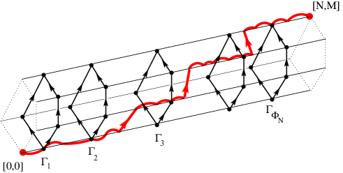
Figure 2: The skeleton for the slab graph and a longest path.

We have $\mathbb{E}(\Gamma_{2}-\Gamma_{1})=1/\lambda$. If

$$\Phi_{n}:=|\SS\cap[0,n]|,$$

we have $\lim_{n\to\infty}\Phi_{n}/n=\lambda$, a.s. Furthermore, $C=\lambda\mathbb{E}L[\Gamma_{1},\Gamma_{2}]\leq 1$. Condition [D2^′] implies that $\mathbb{E}(\Gamma_{2}-\Gamma_{1})^{2}<\infty$ and hence $\mathbb{E}L^{(i)}[\Gamma_{2}-\Gamma_{1}]^{2}<\infty$. By Corollary 1, the random variables

$$\big{(}\Gamma_{2}-\Gamma_{1},~{}L^{(i)}[\Gamma_{1},\Gamma_{2}]\big{)},~{}~{}\big{(}\Gamma_{3}-\Gamma_{2},~{}L^{(i)}[\Gamma_{3},\Gamma_{2}]\big{)},~{}~{}\ldots$$

are i.i.d., and since $\SS$ is obtained by independent thinning of $\cap_{i\in I}\SS^{(i)}$, we further have that the rows of the last display are also independent when $i$ ranges in $I$.

Consider next a path $\iota=(\iota_{0},\iota_{1},\ldots,\iota_{r})$, of length $|\iota|=r$ in the Hasse diagram $H(I,\preceq)$ and define the quantities

$$L^{*}(\iota)_{n} :=\max_{1\leq j_{0}\leq j_{1}\leq\cdots\leq j_{r}=n}\{L^{(\iota_{0})}[\Gamma_{1},\Gamma_{j_{0}}]+L^{(\iota_{1})}[\Gamma_{j_{0}},\Gamma_{j_{1}}]+\cdots+L^{(\iota_{r})}[\Gamma_{j_{r-1}},\Gamma_{j_{r}}]\}$$

$$L^{*}_{n} :=\max_{\iota}L^{*}(\iota)_{n},$$

where the last maximum is taken over all paths $\iota$ from the minimum to the maximum element of the Hasse diagram.

We now argue that the quantity of interest $L_{n}$ is of order $L^{*}_{n}+o_{\mathrm{d}}(1)$ when $n$ is large by providing an upper and a lower bound. The key observation is that when $n$ is large, the number of points $\Gamma_{j}\leq n$ grows at a positive rate (and hence to infinity). At each of these points, say $\Gamma_{j}$, the graph $G[\Gamma_{j},\Gamma_{j}]$ (being a vertical slice of $G$–see Figure 2) is precisely the Hasse diagram:

$$G[\Gamma_{j},\Gamma_{j}]=H(I,\preceq),\quad j\in\mathbb{Z}.$$

Fix $\iota^{\prime}\prec\iota^{\prime\prime}$ in $I$. Since $\Gamma_{j}$ is a point in the skeleton of $G^{(\iota^{\prime})}$, any $x\leq\Gamma_{j}$ is connected to $\Gamma_{j}$ in $G^{(\iota^{\prime})}$. Similarly, $\Gamma_{j}$ is connected to any $y$ in $G^{(\iota^{\prime\prime})}$. Since $\iota^{\prime}$ is connected to $\iota^{\prime\prime}$ in $G[\Gamma_{j},\Gamma_{j}]$, it follows that, almost surely, there is path in $G$ from any $(x,\iota^{\prime})$ to any $(y,\iota^{\prime\prime})$, if $x\leq\Gamma_{j}\leq y$ for some $\Gamma_{j}\in\SS$ and if $\iota^{\prime}\prec\iota^{\prime\prime}$.

Assume that $\Phi_{n}\geq 2$. Let $\iota=(\iota_{0},\iota_{1},\ldots,\iota_{r})$ be a path in $H(I,\preceq)$ with $\iota_{0}=0$, $\iota_{r}=M$ and consider integers

$$1\leq j_{0}\leq j_{1}\leq\cdots\leq j_{r-1}\leq j_{r}=\Phi_{n}.$$ (35)

Keep in mind that

$$\Gamma_{\Phi_{n}}\leq n.$$

By the construction of the set $\SS$, the following is true:

$$(\Gamma_{1},0)=(\Gamma_{1},\iota_{0})\leadsto(\Gamma_{j_{0}},\iota_{0})\leadsto(\Gamma_{j_{0}},\iota_{1})\leadsto(\Gamma_{j_{1}},\iota_{1})\leadsto\cdots\leadsto(\Gamma_{j_{r-1}},\iota_{r})\leadsto(\Gamma_{j_{r}},\iota_{r})=(\Gamma_{\Phi_{n}},M),$$

where $(x,\iota^{\prime})\leadsto(y,\iota^{\prime\prime})$ means that there is a path from $(x,\iota^{\prime})$ to $(y,\iota^{\prime\prime})$ in $G$. Therefore

$$L_{n}\geq L^{(\iota_{0})}[\Gamma_{1},\Gamma_{j_{0}}]+L^{(\iota_{1})}[\Gamma_{j_{0}},\Gamma_{j_{1}}]+\cdots+L^{(\iota_{r})}[\Gamma_{j_{r-1}},\Gamma_{j_{r}}],$$

because the right-hand side is a lower bound on the length of the specific path chosen in the last display. By keeping $\iota$ fixed and maximising over the $j_{0},\ldots,j_{r}$ satisfying (35) we obtain $L_{n}\geq L^{*}(\iota)_{n}$, and by maximising over $\iota$ we obtain the lower bound

$$L_{n}\geq L^{*}_{\Phi_{n}}.$$

To obtain an upper bound, let $\pi^{*}$ be a path that achieves the maximum in $L_{n}$. Assume that $\Phi_{n}\geq 1$ so that, by the key observation above, $(0,0)$ is connected to $(n,M)$ in $G$. See Figure 3. Hence $\pi^{*}$ is necessarily a path from $(0,0)$ to $(n,M)$.

Let

$$0=\iota_{0}\prec\iota_{1}\prec\cdots\prec\iota_{s}=M$$

be the distinct values of the $I$-components of the elements of $\pi^{*}$ in order of appearance in $\pi^{*}$. (The sequence $(\iota_{0},\iota_{1},\ldots,\iota_{s})$ is not necessarily a path in $H(I,\preceq)$.) So for each $k=0,\ldots,s-1$, there are vertices $(x_{k},\iota_{k})$, $(y_{k},\iota_{k+1})$ which are consecutive in the path $\pi^{*}$.

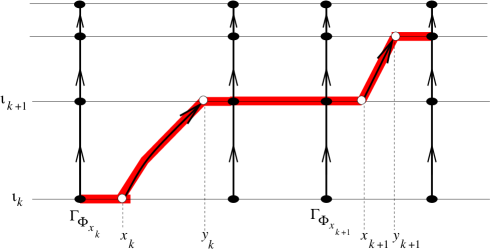
Figure 3: Construction used in obtaining the upper bound.

Hence

$$x_{k}\leq y_{k}\leq x_{k+1},\quad\text{ for all }k=0,1,\ldots,s-1,$$

where, by convention, we set $x_{s}=n$. The point of $\SS$ prior to $x_{k}$ is $\Gamma_{\Phi_{x_{k}}}$ and, since $\pi^{*}$ has maximum length, $(\Gamma_{\Phi_{x_{k}}},\iota_{k})$ is an element of $\pi^{*}$. By the maximality of $\pi^{*}$ again, we have that $x_{k}$ and $y_{k}$ are contained between two successive points of $\SS$ (otherwise we would be able to strictly increase the length of the path). Hence

$$\Gamma_{\Phi_{x_{k}}}\leq x_{k}\leq y_{k}\leq\Gamma_{1+\Phi_{x_{k}}}\leq x_{k+1},\quad\text{ for all }k=0,1,\ldots,s-1.$$ (36)

We thus have

$$L_{n}=|\pi^{*}|=L^{(\iota_{0})}[0,\Gamma_{1}]+L^{(\iota_{0})}[\Gamma_{1},\Gamma_{\Phi_{x_{0}}}]+\sum_{k=0}^{s-1}\bigg{\{}L^{(\iota_{k})}[\Gamma_{\Phi_{x_{k}}},x_{k}]+1+L^{(\iota_{k+1})}[y_{k},\Gamma_{\Phi_{x_{k+1}}}]\bigg{\}}+L^{(\iota_{s})}[\Gamma_{\Phi_{n}},n].$$

Due to (36), we have

$$L^{(\iota_{k})}[\Gamma_{\Phi_{x_{k}}},x_{k}] \leq L^{(\iota_{k})}[\Gamma_{\Phi_{x_{k}}},\Gamma_{1+\Phi_{x_{k}}}],$$ (37)

$$L^{(\iota_{k+1})}[y_{k},\Gamma_{\Phi_{x_{k+1}}}] \leq L^{(\iota_{k+1})}[\Gamma_{\Phi_{x_{k}}},\Gamma_{\Phi_{x_{k+1}}}],\quad k=0,\ldots,s-1.$$ (38)

Moreover,

$$L^{(\iota_{0})}[0,\Gamma_{1}] \leq L^{(\iota_{0})}[\Gamma_{0},\Gamma_{1}]$$ (39)

$$L^{(\iota_{s})}[\Gamma_{\Phi_{n}},n] \leq L^{(\iota_{s})}[\Gamma_{\Phi_{n}},\Gamma_{1+\Phi_{n}}].$$ (40)

Each of the right-hand sides of (37), (39) and (40) is bounded above by $\max_{0\leq j\leq\Phi_{n}}L^{(\iota)}[\Gamma_{j},\Gamma_{1+j}]$. If we then define

$$\zeta_{n}:=\sum_{\iota\in I}\max_{0\leq j\leq\Phi_{n}}L^{(\iota)}[\Gamma_{j},\Gamma_{1+j}]$$

and use (38), we obtain

$$L_{n}\leq\zeta_{n}+M+\sum_{k=0}^{s-1}L^{(\iota_{k+1})}[\Gamma_{\Phi_{x_{k}}},\Gamma_{\Phi_{x_{k+1}}}].$$

Since for each sequence $0=\iota_{0}\prec\iota_{1}\prec\cdots\prec\iota_{s}=M$ of distinct ordered elements of $I$ we can find a path in the Hasse diagram containing these elements, it follows easily that

$$L_{n}\leq\zeta_{n}+M+L_{\Phi_{n}}^{*},$$

which gives the upper bound. The upper bound is close to $L_{n}$ in the sense that the sequence the $\zeta_{n}$ are of order 1 in distribution, i.e. that $(\zeta_{n})$ is tight random sequence. On the other hand, $nt=\Gamma_{\Phi_{[nt]}}-\Gamma_{1}+o_{\mathrm{d}}(1)$. It is thus clear that the weak limit of $\ell_{n}$ and that of

$$\ell^{*}_{n}(t):=\frac{L^{*}_{\Phi_{[nt]}}-C(\Gamma_{\Phi_{[nt]}}-\Gamma_{1})}{\kappa\sqrt{n}},\quad t\geq 0,$$

if it exists, will be identical. Setting

$$\ell^{*\!*}_{n}(t):=\frac{L^{*}_{[nt]}-C(\Gamma_{[nt]}-\Gamma_{1})}{\kappa\sqrt{n}},\quad\varphi_{n}(t):=\frac{\Phi_{[nt]}}{n},$$

we have

$$\ell^{*}_{n}(t)=\ell^{*\!*}_{n}(\varphi_{n}(t)),$$ (41)

and so the weak limit of $\ell_{n}^{*}$ is equal to that of $\ell_{n}^{*\!*}$ (if this exists) composed by the function $\{\lambda t\}$.

To show that the weak limit of $\ell_{n}^{*}$ exists and find it, define the function $\psi:D[0,\infty)^{I}\to D[0,\infty)$ by

$$\psi(\beta^{(i)},i\in I)(t):\max_{\iota}~{}\sup_{\begin{subarray}{c}0\leq t_{0}\leq t_{1}\leq\cdots\leq t_{r}=t\\ |\iota|=r\end{subarray}}\bigg{\{}\beta^{(\iota_{0})}(t_{0})+\big{[}\beta^{(\iota_{1})}(t_{1})-\beta^{(\iota_{1})}(t_{0})\big{]}+\cdots\\ \cdots+\big{[}\beta^{(\iota_{r})}(t_{r})-\beta^{(\iota_{r})}(t_{r-1})\big{]}\bigg{\}}$$

where the maximum is taken over all paths $\iota$ from the minimum to the maximum element in the Hasse diagram $H(I,\preceq)$. The function $\psi$ is continuous (with respect to the topology of uniform convergence). Let

$$s^{(i)}_{n}(t):=\frac{L^{(i)}[\Gamma_{1},\Gamma_{[nt]}]-C(\Gamma_{[nt]}-\Gamma_{1})}{\sigma\sqrt{n}},\quad t\geq 0,\quad i\in I,$$

where

$$\sigma^{2}:=\operatorname{var}\{L^{(i)}[\Gamma_{1},\Gamma_{2}]-C(\Gamma_{2}-\Gamma_{1})\}$$

Since $L^{(i)}[\Gamma_{j},\Gamma_{j+1}]$, $j\geq 1$, $i\in I$ are i.i.d. with common variance $\sigma^{2}$ we have (Theorem 2) that

$$\big{(}s_{n}^{(i)},i\in I\big{)}\Rightarrow\big{(}B^{(i)},i\in I\big{)}$$ (42)

where $B^{(i)}$, $i\in I$ are i.i.d. standard Brownian motions. Let

$$\kappa:=\lambda^{1/2}\sigma$$

and observe that

$$\ell_{n}^{*\!*}(t)=\lambda^{-1/2}\cdot\psi(s_{n}^{(i)},i\in I)(t).$$

By (42) and the invariance principle,

$$\ell_{n}^{*\!*}\Rightarrow\lambda^{-1/2}\cdot\psi(B^{(i)},i\in I).$$

By the relation (41) and the remark following it, we have

$$\ell_{n}^{*}\Rightarrow\psi(B^{(i)},i\in I),$$

and the right-hand side is equal in distribution to $Z$ (defined by (33)-(34)). ∎

The remarks at the end of Section 7 also apply in the current case. We can easily conclude that $T_{n}$, the maximum length of all paths from $(0,0)$ to $(n,M)$, has the same asymptotics as $L_{n}$. In particular, Theorem 5 holds if we replace $L_{n}$ by $T_{n}$.

10 Connection to last passage percolation

Consider now the case

$$I=\{0,1,\ldots,M\}$$

with the usual ordering. Assumption [D3] can be substituted by
          [D3’]   For all $1\leq i\leq M$ we have $r_{0,i-1,i}>0$.
Let $G_{M}$ be the corresponding random directed cylinder graph, referred to as slab graph here. In particular, we can think of $G_{M}$ as the restriction of a graph $G_{\infty}$ on the vertex set $\mathbb{Z}\times\mathbb{Z}_{+}$ where two vertices $(x,i)$ and $(y,j)$, with $(x,i)\bm{<}\!\!\!\!\;\!\!\bm{<}(y,j)$, are connected with probability $p_{y-x,j-i}$ that depends on the relative position of the two vertices on the 2-dimensional lattice.

The problem here becomes that of a last passage percolation , although the model is not the standard nearest-neighbour one. Physically, we can think of tunnels which run upwards (or in directions southwest to northeast) and fluid moving in tunnels. It takes one unit of time to cross a specific tunnel. We are interested in the particle that starts from $(0,0)$ and reaches $(n,M)$ in the largest possible time. Since the Hasse diagram of the set $\{0,1,\ldots,M\}$ with the natural ordering is the linear graph with edges from $i-1$ to $i$, $1\leq i\leq M$, the limit process $Z$ is given by the simplified expression

$$Z_{t}=\max_{0\leq t_{0}\leq\cdots\leq t_{M}=t}\big{\{}B^{(0)}(t_{0})+[B^{(1)}(t_{1})-B^{(1)}(t_{0})]+\cdots+[B^{(M)}(t_{M})-B^{(M)}(t_{M-1})]\big{\}},\quad t\geq 0.$$

The latter process is a Brownian last passage percolation process. As was shown in [6, 21, 32] it is a non-Gaussian process with marginal distribution

$$Z_{t}\stackrel{{\scriptstyle\text{d}}}{{=}}\sqrt{t}\cdot\lambda_{M},$$

for each $t\geq 0$, where $\lambda_{M}$ is the largest eigenvalue of a random $(M+1)\times(M+1)$ Gaussian Unitary Ensemble (GUE) [29].

Tracy and Widom [34, 35] showed that, as $M\to\infty$, the following weak limit holds:

$$M^{1/6}(\lambda_{M}-2\sqrt{M})\Rightarrow F_{\text{TW}},$$

with $F_{\text{TW}}$ being the Tracy-Widom distribution whose hazard rate equals $\int_{t}^{\infty}q(x)^{2}dx$, where $q(x)$ satisfies a Painlevé II equation; see [2, eq. (3.1.7)]. For an account on the universality of this distribution, see, e.g., [17]. A number of interesting results have been proved relating this limiting distribution with certain stochastic models. These models include longest increasing subsequence [5], last passage percolation, non-colliding particles, tandem queues [6, 21], and random tilings [24]. For the last passage percolation, in particular, this limit is known to appear in two cases. The first is the Brownian last passage percolation. The second is the last passage percolation model with exponential (or geometric) weights. In this model one puts independent and identically distributed exponential random variables in the vertices of $\mathbb{Z}_{+}^{2}$ and considers the maximum $L(M,N)$ of the sums of the weights over all directed paths from $(0,0)$ to $(M,N)$. It was shown in [23] the random variable $L(N,N)$, properly normalized, converges to the Tracy-Widom distribution as $N$ goes to infinity. In [8], more general weights were considered and an analogous result for the random variable $L(N,N^{a})$ (for an appropriate $a$ depending on moment conditions) was obtained. It is then natural to conjecture that a similar phenomenon occurs in our slab graph too.

Denis Denisov
School of Mathematics
Cardiff University
Cardiff CF24 4AG, UK
E-Mail: dennissov@googlemail.com

Serguei Foss
School of Mathematical Sciences
Heriot-Watt University
Edinburgh EH14 4AS, UK
E-mail: foss@ma.hw.ac.uk

Takis Konstantopoulos
School of Mathematical Sciences
Heriot-Watt University
Edinburgh EH14 4AS, UK
E-mail: takiskonst@gmail.com

References

- [1] Alon, N., Bollobás, B., Brightwell, G., and Janson, S. (1994) Linear extensions of a random partial order. Ann. Prob. 4, 108-123.
- [2] Anderson, G. W., Guionnet, A. and Zeitouni, O. (2010) An Introduction to Random Matrices. Cambridge Univ. Press, Cambridge.
- [3] Baik, J. (2008) Limiting distribution of last passage percolation models. arXiv:math/0310347v2
- [4] Barak, A.B. and Erdős, P. (1984) On the maximal number of strongly independent vertices in a random acyclic directed graph. SIAM J. Algebr. Discr. Methods 5, 508-514.
- [5] Baik, J., Deift, P. and Johansson, K. (1999) On the distribution of the length of the longest increasing subsequence of random permutations. J. Amer. Math. Soc. 12, 1119–1178.
- [6] Baryshnikov, Y., (2001). GUEs and queues. Probab. Theory Related Fields 119, 256-274.
- [7] Billingsley, P. (1968) Convergence of Probability Measures. Wiley, New York.
- [8] Bodineau, T. and Martin, J. (2005). A universality property for last-passage percolation paths close to the axis. Electron. Comm. Probab. 10, 105-112.
- [9] Borovkov, A.A. (1978) Ergodicity and stability theorems for a class of stochastic equations and their applications. Theory Prob. Appl. 23, 227-258.
- [10] Borovkov, A.A. (1980) Asymptotic Methods in Queueing Theory. Nauka, Moscow (Russian edition). Revised English edition: Wiley, New York, 1984.
- [11] Borovkov, A.A. (1998) Ergodicity and Stability of Stochastic Processes. Wiley, Chichester.
- [12] Borovkov, A.A. and Foss, S.G. (1992) Stochastically recursive sequences and their generalizations. Sib. Adv. Math. 2, n.1, 16-81.
- [13] Borovkov, A.A. and Foss, S.G. (1994) Two ergodicity criteria for stochastically recursive sequences. Acta Appl. Math. 34, 125-134.
- [14] Cohen, J.E. and Newman, C.M. (1991) Community area and food chain length: theoretical predictions. Amer. Naturalist 138, 1542-1554.
- [15] Comets, F., Fernández, R. and Ferrari, P.A. (2002). Processes with long memory: regenerative construction and perfect simulation. Ann. Appl. Probab. 12, 921-943.
- [16] Davey, B.A. and Piestley, H.A. (1990). Introduction to Lattices and Order. Cambridge University Press, Cambridge.
- [17] Deift, P. (2006) Universality for mathematical and physical systems. Proc. Intern. Congress of Mathematicians, Madrid, Vol. 1, 125-152.
- [18] Foss, S. and Konstantopoulos, T. (2003) Extended renovation theory and limit theorems for stochastic ordered graphs. Markov Process. Related Fields 9, n. 3, 413–468.
- [19] Foss, S. and Tweedie, R.L. (1998) Perfect simulation and backward coupling. Stochastic Models 14, No. 1-2, 187-204.
- [20] Foss, S., Tweedie, R.L. Corcoran. J.N. (1998) Simulating the Invariant Measures of Markov Chains using Backward Coupling at Regeneration Time. Probability in the Engineering and Informational Sciences 12, 303-320.
- [21] Gravner, J., Tracy, C. A. and Widom, H., (2001). Limit theorems for height fluctuations in a class of discrete space and time growth models. J. Statist. Phys. 102, 1085-1132.
- [22] Isopi, M. and Newman, C.M. (1994) Speed of parallel processing for random task graphs. Comm. Pure and Appl. Math 47, 261-276.
- [23] Johansson, K (2000). Shape fluctuations and random matrices. Comm. Math. Phys. 209, no. 2, 437–476.
- [24] Johansson, K (2005). The arctic circle boundary and the Airy process. Ann. Prob. 33, 1-30.
- [25] Kallenberg, O. (1992) Foundations of Modern Probability, Springer-Verlag, New York.
- [26] Lindvall, T. Lectures on the Coupling Method. Wiley, New York.
- [27] Martin, J. B. (2004) Limiting shape for directed percolation models. Ann. Prob. 32, 2908-2937.
- [28] Martin, J. B. (2006) Last-passage percolation with general weight distribution. Markov Processes and Related Fields 12, 273-299.
- [29] Mehta, M. (2004) Random matrices, Third edition, Pure and Applied Mathematics (Amsterdam), 142. Elsevier/Academic Press, Amsterdam.
- [30] Newman, C.M. (1992) Chain lengths in certain random directed graphs. Random Structures and Algorithms 3, No.3, 243-253.
- [31] Newman, C.N. and Cohen, J.E. (1986) A stochastic theory of community food webs: IV. Theory of food chains in large webs. Proc. R. Soc. London Ser. B 228, 355-377.
- [32] O’Connell, N. and Yor, M., (2002) A representation for non-colliding random walks. Electron. Comm. Probab. 7, 1-12.
- [33] Prop, J. and Wilson, D. (1997) Coupling from the past: a user’s guide. In: Microsurveys in discrete probability: DIMACS workshop, June 2-6, 1997. American Math. Society.
- [34] Tracy, C.A. and Widom, H. (1993) Level-spacing distributions and the Airy kernel. Physics Letters B 305, 115-118.
- [35] Tracy, C.A. and Widom, H. (1994) Level-spacing distributions and the Airy kernel. Comm. Math. Physics 159, 151–174.