Abstract

Using the flux compactification scenario in a generic supergravity model we propose a set of conditions which will generate de-Sitter or anti de-Sitter vacua for appropriate choices of the parameters in superpotential. It is shown that a mass spectrum consistent with softly broken TeV scale supersymmetry in a minimal supersymmetric standard model at the observable sector can be obtained along with a tiny cosmological constant when the Kähler and superpotential of the hidden sector satisfy a set of general constraints. Constructing a specific model which satisfy the above constraints, it is demonstrated that all the hidden sector fields have vacuum expectation values close to Planck scale and the resulting low energy potential does not have any flat direction.

1 Introduction

Supersymmetry(susy) has emerged as one of the leading candidates for unraveling the physics beyond the Standard Model(SM). The most challenging and longstanding questions in the context of supersymmetric theories are related to the mechanism of supersymmetry breaking. The need for susy breaking originates from the fact that no superparticle has yet been observed in nature. The fine tuning/gauge hierarchy problem points towards the requirement of the susy breaking scale being close to TeV so that the Higgs mass does not receive radiative corrections beyond TeV. As a result TeV scale supersymmetric theories have drawn special attentions in view of the forthcoming results in the LHC. A possible origin of these symmetry breaking terms can be understood by embedding MSSM in a supergravity theory (SUGRA)[1, 2, 3]. Supergravity theories drew further attention when they were shown to emerge as low energy effective theories of underlying string theories which can take care of the renormalizability problems persistent in the supergravity models.

In a plethora of supergravity models supersymmetry is assumed to be spontaneously broken at a high energies ($\sim 10^{11}~{}\rm GeV$) via the vacuum expectation value(VEV) of the $F$ or $D$ terms [4, 5, 6, 7, 8]. Some realistic models of spontaneous susy breaking requires two different sets of superfields, one of which participate in Standard Model gauge interactions and the other consists of singlets under the SM gauge group. The singlet fields usually have very large VEV and constitute the hidden sector of the theory. Such a sector has it’s natural origin in the framework of string theory. In a formalism where the matter fields of the MSSM constituting the observable sector are assumed to couple with the hidden sector singlets via gravitational interactions, spontaneous susy breaking in the hidden sector results into generation of soft-susy breaking terms in the observable sector[4, 5]. If the local susy breaking is expected at a scale $\Lambda$, the soft terms would have a scale of order $\Lambda^{2}/M_{p}$, where $M_{p}$ is the Planck mass. Considering $\Lambda\sim 10^{11}~{}\rm GeV$, soft supersymmetry breaking terms $\sim$ TeV can be produced at the observable sector. Supergravity models however are often encountered with the existence of flat directions in the hidden sector. It is therefore necessary to lift the flat directions by appropriate mechanism.

While normally SUSY breaking leads to appearance of non-vanishing vacuum energy, some of the of the SUGRA models may have broken SUSY with vanishing vacuum energy. The experimental data indeed indicates a near-flatness of the present universe [11] with a vanishingly small vacuum energy. Simple model like no-scale supergravity scenario can give plausible explanation for nearly vanishing vacuum energy. However these models have limitations to produce viable susy phenomenology at low energies($\sim$TeV) [13, 14]. Therefore the search for a near-Minkowski/de-Sitter vacua has attracted considerable interest in recent years. In this regard various supergravity and string motivated models generating de-Sitter vacua at the TeV scale have been proposed [15, 16, 17, 18, 19, 20, 21, 22, 23, 24, 25, 26, 27, 28, 29, 30]. Substantial progress have been made in this direction by a model developed in 2003[15] in the context of string theory known as the KKLT model. This was followed by a plethora of propositions [17, 20, 21, 23, 31, 24, 25, 26, 27]which revolve around building an effective description of low energy physics through a superpotential generated by background fluxes and a convenient choice of Kähler potential motivated by a suitable compactification scheme arising in String/M-Theory.

In this backdrop we address the following question in the present article :

• What are the general set of criteria that the Kahler and superpotential of a supergravity model have to satisfy to produce a viable phenomenology at the Tev scale so that there is no flat direction in the model and the effective vacuum energy at the low energy is tiny and positive which is compatible to the present day observation?

Adapting the technique proposed in [15] an additional moduli field is incorporated in both the superpotential and the Kähler potential. As can be seen latter, this extra moduli field is crucial in producing small vacuum energy, once susy is broken at the hidden sector. A small vacuum energy at the minimum and viable susy breaking terms at the observable sector restrict the choice of the Kähler and the superpotential. The order of magnitude of the gravitino mass and the soft susy breaking parameters namely the soft scalar mass, and the coefficient of the trilinear and the bilinear terms are estimated. This set-up is later illustrated with a toy model.

In section (1.1) of this article a brief review of [15] is presented. In section (2) an extension of the same has been suggested. Section (3) provides the extremization condition for the scalar potential. Section (4) deals with the estimation of soft susy breaking parameters. In section (5) a possible model is proposed in support of our analysis. Section (6) is devoted to summarizing the work.

1.1 KKLT set-up : a quick revisit

In this section a brief review of some parts of the KKLT proposal relevant to the present work is presented. We begin with a quick revisit to the basic frame work of $\mathcal{N}=1$ supergravity. As mentioned in the introduction, the complete Lagrangian (up to two derivatives) in $\mathcal{N}=1$ supergravity is specified by chiral superfields $\phi_{M}$ of the theory where the index $M$ runs over the entire set of chiral superfields, the analytic gauge-kinetic function $f_{\alpha}(\phi_{M})$, and the real gauge-invariant Kähler function $G(\phi_{M},{\phi_{M}}^{*})$. The dimensionless function $G$ is defined in terms of Kähler potential $K(\phi_{M},{\phi_{M}}^{*})$ and superpotential $W(\phi_{M})$ as,

$$G(\phi_{M},{\phi_{M}}^{*})=\frac{K(\phi_{M},{\phi_{M}}^{*})}{M_{p}^{2}}+\log\mid\frac{W(\phi_{M})}{M_{p}^{3}}\mid^{2}{\bf{\color[rgb]{0,0,1}\textsf{,}}}$$ (1)

where $M_{p}\sim 10^{19}~{}\rm GeV$ denotes the Planck scale. The tree level(F-part) supergravity scalar potential in the Einstein frame is given by

$$V(\phi_{M},{\phi_{M}}^{*})=e^{K/M_{p}^{2}}\left(K^{I\bar{J}}D_{I}WD_{\bar{J}}W^{*}-\frac{3}{M_{p}^{2}}\mid W(\phi_{M})\mid^{2}\right).$$ (2)

Here $D_{I}W=\partial_{I}W+\frac{K_{I}}{M_{p}^{2}}W$ is the Kähler covariant derivative of the superpotential and $K_{I{\bar{J}}}={\partial}_{\bar{J}}{\partial}_{I}K$ is the Kähler metric. Now, using $F^{M}=M^{3}_{p}e^{G/2}K^{M\bar{P}}G_{\bar{P}}$ the scalar potential can be recast as

$$V(\phi_{M},{\phi_{M}}^{*})=\left(\bar{F}^{\bar{N}}K_{\bar{N}M}F^{M}-3M_{p}^{4}e^{G}\right).$$ (3)

In type-IIB String theory de-Sitter solutions are forbidden in the leading order of $\alpha^{\prime}$ (the string tension) and $g_{s}$ (the string coupling) by a no-go theorem [16]. So a natural way of finding a de-Sitter solution in string theory is to include corrections from higher order in $\alpha^{\prime}$ and $g_{s}$ to the no-scale structure. In [15] this objective is achieved in a two fold way :

1. In the presence of a non-zero flux the Calabi-Yau moduli combines suitably to form a superpotential of the form

   $$W=\int_{M}G_{3}\wedge\Omega=\int_{M}(F_{3}-\tau H_{3})\Omega$$ (4)

   where $H_{3}$ and $F_{3}$ are the NS-NS and R-R three-form fluxes and $\tau$ is the axion-dilaton of type-IIB string theory. The Kähler structure of the internal manifold (Calabi-Yau four-fold) is encoded in a Kähler potential whose tree-level form is

   $${K}=M^{2}_{p}(-3ln[-i(\rho-\overline{\rho})]-ln[-i(\tau-\overline{\tau})]-ln[\int_{M}\Omega\wedge\overline{\Omega}]),$$ (5)

   where $\rho$ is the single volume modulus.

   This structure however does not admit any de-Sitter solution and therefore calls for inclusion of corrections to the leading order. The relevant correction terms can be attributed to two different sources. One of these, being instanton correction which at large volume of the internal four-fold yields an additional term to the Superpotential

   $${W_{inst}}=P(z_{i})e^{2\pi i\rho}.$$ (6)

   While $P(z_{i})$ is the holomorphic one-loop determinant, the leading order in the exponential originates from the action of Euclidean $D3$-branes wrapping on a four-cycle. With all other moduli fixed, they can be integrated out to produce an effective superpotential for $\rho$ alone.

   The origin of the other correction is described as follows. In type II-B string theory compactified on a Calabi-Yau fourfold a stack of $N$ number of D7 branes wrapping on 4-cycles in the compact manifold gives rise to non-abelian gauge groups. The effective low-energy $\mathcal{N}=1$ supersymmetric theory undergoes gluino condensation resulting into a superpotential,

   $$W_{gauge}=\Lambda_{N}^{3}=Ae^{\frac{2\pi i\rho}{N}}.$$ (7)

   Here $\Lambda_{N}$ is the dynamical scale of gauge theory. The coefficient $A$ can be determined by the energy scale below which Supersymmetric QCD is valid. Plugging $\rho=iT$ in the superpotential along with a logarithmic $T$ dependence in the Kähler potential we arrive at,

   $$W=W_{0}+Ae^{-a\tilde{T}}~{},~{}~{}~{}K=-3M_{p}^{2}\log(\tilde{T}+\tilde{T}^{*}),$$ (8)

   where $\tilde{T}=\frac{T}{M_{p}}$.
   In a supersymmetric vacuum $D_{T}{W}=0$. The axion field in $\rho$ is set to zero for the sake of simplification. $\{A,a,W_{0}\}$ is taken to be real and $W_{0}$ to be negative. The condition for susy preserving vacua corresponds to the minimum of the scalar potential determined by the VEV of $T$.

   $$D_{T}W=0\Longrightarrow W_{0}=-Ae^{-a\tilde{t_{0}}}(1+\frac{2}{3}a\tilde{t_{0}}).$$ (9)

   Here $\tilde{t}_{0}$ denotes the VEV of $\tilde{T}$. This makes the scalar potential (2) negative at the minimum and can be given by,

   $$V_{AdS}=-(3e^{K/M_{p}^{2}}{W}^{2}/M_{p}^{2})_{AdS}={\frac{1}{M_{p}^{2}}}\frac{-a^{2}A^{2}e^{-2a\tilde{t_{0}}}}{6\tilde{t_{0}}}$$ (10)

   Thus a supersymmetry preserving AdS minimum has been generated. Fixing the values of $\{A,a,W_{0}\}$, one can estimate the VEV of the moduli $T$ via (9) which in turn determines the $V_{AdS}$ through (10).

2. The next important step is to add a de-Sitter lifting term to the scalar potential. The principal issue is to allow for generation of some extra energy from the flux background which shows up in the scalar potential as an extra term namely $D/T^{3}$. This is achieved by incorporating anti $D3$-branes ($\overline{D3}$-branes) in the picture. The coefficient D depends on the number of $\overline{D3}$-branes introduced. The introduction of $\overline{D3}$-brane breaks supersymmetry and the results in a positive definite vacuum energy by compensating the AdS value of the scalar potential at the minimum. Moreover, by fine-tuning $D$, one can have a dS minimum close to zero.

We now employ the basic philosophy employed in KKLT model to the $4d$, $\mathcal{N}=1$ supergravity to investigate the issue of small and positive cosmological constant with the generation of soft susy breaking terms at the TeV scale. In the present context, we restrict ourselves to the tree level contribution of the cosmological constant, while it is possible to limit the effect of radiative corrections in this computation[32]. We will show how the Kähler correction may lead to the AdS/dS nature of the scalar potential.

2 An Extended Scenario

In this section a scenario in the context of $4d$, $\mathcal{N}=1$ supergravity is constructed with an AdS minimum where supersymmetry is broken at an intermediate energy scale (lower than the Planck scale and higher than the TeV scale). In this construction $\Phi_{M}$ is assumed to run over the superfields in the hidden sector as well as in the observable sector. The superpotential and Kähler potential which represent the hidden sector contributions are denoted by $\hat{W}$ and $\hat{K}$.

While generating the small AdS minimum at the hidden sector, we will now try to address the following question in context of the present scenario vis-a-vis the KKLT model on a very general ground.

• Does the inclusion of the extra modulus in the set-up improves our understanding of the intermediate local supersymmetry breaking and helps to generate a vanishingly small positive cosmological constant as well as viable susy breaking terms at the observable sector?

In seeking a probable answer to this question an additional hidden sector moduli $S$ is inserted in the superpotential and Kähler potential (8). In particular, the additional term in the superpotential is intended for providing an mechanism for susy breaking at the intermediate scale. The modified superpotential assumes the form,

$$\hat{W}=W_{0}+Ae^{-a\tilde{T}}+f(\tilde{S}).$$ (11)

In the present set-up the tree level Kähler potential may receive corrections from various sources, e.g string loop correction (higher order in $\alpha^{\prime}$ and $g_{s}$). With this possibility in mind a correction term $h(\tilde{T}+\tilde{T}^{*})$ is appended to the tree level Kähler potential. It turns out that the correction term has a crucial role to play in determining the AdS nature of the potential. The corrected Kähler potential has the form,

$$\hat{K}=M_{p}^{2}\left[-3\log(\tilde{T}+\tilde{T}^{*})-\log(\tilde{S}+\tilde{S}^{*})+h(\tilde{T}+\tilde{T}^{*})\right],$$ (12)

Where $\tilde{S}=\frac{S}{M_{p}}$ and $\tilde{T}=\frac{T}{M_{p}}$. For these choices, the scalar potential (3) can be written as,

$$V_{h}=\frac{1}{M_{p}^{2}}\frac{e^{h}}{16\tilde{s}\tilde{t}^{3}}\left[4\tilde{s}^{2}\left[f^{\prime}(\tilde{s})-\frac{\hat{W}}{2\tilde{s}}\right]^{2}+\frac{1}{(\frac{3}{4\tilde{t}^{2}}+h^{\prime\prime})}\left[aAe^{-a\tilde{t}}+\hat{W}\left(\frac{3}{{2\tilde{t}}}-h^{\prime}\right)\right]^{2}-3\hat{W}^{2}\right].$$ (13)

Here, $V_{h}$ stands for the scalar potential in the hidden sector only, $\tilde{t}$ and $\tilde{s}$ are the real components of the complex moduli $\tilde{T}$ and $\tilde{S}$ respectively. Following [15] we assume $W_{T}=W_{0}+Ae^{-a\tilde{t}}$, with the condition for susy preserving minimum (9),

$$W_{T}=\frac{Aae^{-a\tilde{t}_{0}}}{-\frac{3}{2\tilde{t_{0}}}+h^{\prime}(\tilde{t_{0}})},$$ (14)

Here $t_{0}$ and $s_{0}$ are the VEVs of the real superfield $t$ and $s$ respectively. Remembering that the SUSY breaking at the observable sector at the scale $\Lambda$ ( $\sim$ Tev ) results into positive vacuume energy $\sim$ $\Lambda^{4}$, whereas the observed value is very very tiny, we arrive at the constraint condition

$$(1+\sqrt{3})\left[\frac{Aae^{-a\tilde{t}_{0}}}{-\frac{3}{2\tilde{t}_{0}}+h^{\prime}(\tilde{t}_{0})}+f(\tilde{s}_{0})\right]=2\tilde{s}_{0}f^{\prime}(\tilde{s}_{0}).$$ (15)

The constraint (15) puts restrictions on the parameters and choice of the functions $h$ and $f$. Imposing this constraint condition allows the scalar potential of the hidden sector to be written as,

$$V_{h0}=\frac{1}{M_{p}^{2}}\frac{e^{h}}{16\tilde{s}_{0}\tilde{t}_{0}^{3}}\times\frac{1}{(h^{\prime\prime}(\tilde{t}_{0})+\frac{3}{4\tilde{t}_{0}^{2}})}f^{2}(\tilde{s}_{0})\left(\frac{3}{2\tilde{t}_{0}}-h^{\prime}(\tilde{t}_{0})\right)^{2}.$$ (16)

where $V_{h0}$ is the VEV of the scalar potential(13). Thus the nature of the minimum depends entirely on the choice of the function $h(\tilde{t})$. In the following section an example has been presented in this regard. For a value of $f(\tilde{s})\sim 10^{25}~{}\rm GeV^{3}$ at VEV, vacuum energy $V_{h_{0}}\sim-10^{12}~{}\rm GeV^{4}$ can be produced provided all the dimensionless quantities are of $O(1)$. This, together with the contributions from the observable sector in the scalar potential $V_{obs}\sim 10^{12}~{}\rm GeV^{4}$ may conspire to produce a small but positive cosmological constant.

The above analysis implies that the parameter $A\sim\Lambda_{N}^{3}$ should have a mass scale with $\Lambda_{N}\simeq 10^{14}~{}\rm GeV$ to produce viable soft breaking terms. This will be justified in the following sections. However admitting such large value for $A\sim 10^{42}~{}\rm GeV^{3}$, the condition (15) can only be satisfied if $f^{\prime}(\tilde{s})|_{VEV}\sim A>>f(\tilde{s})|_{VEV}$ holds.

3 Extremization

In this section the issue of the stability of the scalar potential (13) is addressed. The potential is required to satisfy the conditions for global minimum with well-defined VEV for all the fields. In this section the conditions for extremum for (13) are determined for arbitrary $f(\tilde{s})$ and $h(\tilde{t})$ where the constraints (14) and (15) have been used.

The first derivative of (13) with respect to the moduli $\tilde{s}$ yields the condition,

$$\begin{split}\frac{\partial V_{h}}{\partial\tilde{s}}|_{\tilde{s}_{0},\tilde{t}_{0}}=&\frac{1}{16\tilde{s}_{0}^{2}\tilde{t}_{0}^{3}(3+4\tilde{t}_{0}^{2}h^{\prime\prime}[\tilde{t}_{0}])}[(2-\sqrt{3})e^{h[\tilde{t}_{0}]}(4\tilde{s}_{0}^{2}f^{\prime}[\tilde{s}_{0}](-\sqrt{3}f^{\prime}[\tilde{s}_{0}]+(3+\sqrt{3}\tilde{s}_{0}f^{\prime\prime}[\tilde{s}_{0}])\\ &(3+4\tilde{t}_{0}^{2}h^{\prime\prime}[\tilde{t}_{0}])-(2+\sqrt{3})f[\tilde{s}_{0}]^{2}(3+4\tilde{t}_{0}(h^{\prime}[\tilde{t}_{0}](-3+\tilde{t}_{0}h^{\prime}[\tilde{t}_{0}])-2\tilde{t}_{0}h^{\prime\prime}[\tilde{t}_{0}]))\\ &+2\tilde{s}_{0}f[\tilde{s}_{0}](-2(2+\sqrt{3})\tilde{s}_{0}f^{\prime\prime}[\tilde{s}_{0}](3+4\tilde{t}_{0}^{2}h^{\prime\prime}[\tilde{t}_{0}])+f^{\prime}[\tilde{s}_{0}](12+9\sqrt{3}+h[\tilde{t}_{0}]\\ &+(-3(2+\sqrt{3})h^{\prime}[\tilde{t}_{0}]+(2+\sqrt{3})\tilde{t}_{0}h^{\prime}[\tilde{t}_{0}]^{2}-2\tilde{t}_{0}h^{\prime}[\tilde{t}_{0}]))))]=0\end{split}$$ (17)

Similarly the derivative with respect to the moduli field $\tilde{t}$ gives rise to the condition,

$$\begin{split}\frac{\partial V_{h}}{\partial\tilde{t}}|_{\tilde{s}_{0},\tilde{t}_{0}}=&\frac{1}{16\tilde{s}_{0}\tilde{t}_{0}^{4}(3+4\tilde{t}_{0}^{2}h^{\prime\prime}[\tilde{t}_{0}])^{2}}((2-\sqrt{3})e^{h[\tilde{t}_{0}])]}(2(3+\sqrt{3})\tilde{s}_{0}^{2}f^{\prime}[\tilde{s}_{0}]^{2}(-3+2\tilde{t}_{0}h^{\prime}[\tilde{t}_{0}])\\ &(3+4\tilde{t}_{0}^{2}h^{\prime\prime}[\tilde{t}_{0}])^{2}+\tilde{s}_{0}f[\tilde{s}_{0}]f^{\prime}[\tilde{s}_{0}](3+4\tilde{t}_{0}^{2}h^{\prime\prime}[\tilde{t}_{0}])(9(11+7\sqrt{3}+2(1+\sqrt{3})a\tilde{t}_{0})\\ &+2\tilde{t}_{0}(2(1+\sqrt{3})\tilde{t}_{0}(9+2a\tilde{t}_{0})h^{\prime}[\tilde{t}_{0}]^{2}-4(1+\sqrt{3})\tilde{t}_{0}^{2}h^{\prime}[\tilde{t}_{0}]^{3}+6(9+5\sqrt{3})\tilde{t}_{0}h^{\prime\prime}[\tilde{t}_{0}]\\ &-h^{\prime}[\tilde{t}_{0}](3(11+9\sqrt{3}+4(1+\sqrt{3})a\tilde{t}_{0})+4(3+\sqrt{3}\tilde{t}_{0}^{2}h^{\prime\prime}[\tilde{t}_{0}])))\\ &+(2+\sqrt{3})f[\tilde{s}_{0}]^{2}(-27+\tilde{t}_{0}(4\tilde{t}_{0}^{2}h^{\prime}[\tilde{t}_{0}]^{3}(3+4\tilde{t}_{0}^{2}h^{\prime\prime}[\tilde{t}_{0}])\\ &+12\tilde{t}_{0}(-6h^{\prime\prime}[\tilde{t}_{0}]+4\tilde{t}_{0}^{2}h^{\prime\prime}[\tilde{t}_{0}]^{2}-3\tilde{t}_{0}h^{\prime\prime}[\tilde{t}_{0}])\\ &-16\tilde{t}_{0}h^{\prime}[\tilde{t}_{0}]^{2}(3+6\tilde{t}_{0}^{2}h^{\prime\prime}[\tilde{t}_{0}]+\tilde{t}_{0}^{3}h^{\prime\prime\prime}[\tilde{t}_{0}])+3h^{\prime}[\tilde{t}_{0}](27+68\tilde{t}_{0}^{2}h^{\prime\prime}[\tilde{t}_{0}]+16\tilde{t}_{0}^{3}h^{\prime\prime\prime}[\tilde{t}_{0}]))))).\end{split}$$ (18)

Results of the calculation of the second derivatives for suitable choices of $f(\tilde{s})$ and $h(\tilde{t})$ indicates that the conditions stated above can be used to yield a stable global minimum for the scalar potential without having any flat direction. In section (5) with a specific choice of $f(\tilde{s})$ and $h(\tilde{t})$, the existence of a global AdS minimum for the potential will be illustrated.

4 Soft susy breaking parameters

It is worthwhile to discuss the low energy phenomenology encoded in the soft susy breaking parameters. We consider the chiral superfield of $\mathcal{N}=1$ supergravity (see section 1.1) $\Phi_{M}={h_{m},C^{\alpha}}$ where $h_{m}$ corresponds to heavily massive components and constitute the hidden sector and $C^{\alpha}$ are lighter mass components and constitute the observable sector. While the Latin indices run over the entire set of hidden sector fields, the Greek indices denotes the set of the MSSM fields. The superpotential and Kähler potential can be Taylor expanded with respect to the observable sector fields as (for details see [5]).

$$W=\hat{W}(h_{m})+\frac{1}{2}\mu_{\alpha\beta}(h_{m})C^{\alpha}C^{\beta}+\frac{1}{6}Y_{\alpha\beta\gamma}(h_{m})C^{\alpha}C^{\beta}C^{\gamma}+.....$$ (19)

and

$$K=\hat{K}(h_{m},h_{m}^{*})+\tilde{K}_{\bar{\alpha}\beta}(h_{m},h_{m}^{*}){C^{*}}^{\bar{\alpha}}C^{\beta}+\frac{1}{2}(Z_{\alpha\beta}C^{\alpha}C^{\beta}+h.c)+...$$ (20)

As already mentioned the $\hat{W}$ and $\hat{K}$ represent the hidden sector components of the superpotential and Kähler potential. Similarly, in (20) the observable sector Kähler metric is given by $\tilde{K}_{\alpha\bar{\beta}}$. The above expansions for the superpotential and Kähler potential can be plugged in the generic expression for the scalar potential (2) giving rise to the full scalar potential of the theory. Choosing the Kähler metric of the observable sector in diagonal form as

$${\tilde{K}}_{\overline{\alpha}\beta}(h_{m},h_{m}^{*})={\delta}_{\overline{\alpha}\beta}{\tilde{K}}_{\alpha}(h_{m},h_{m}^{*})$$ (21)

and canonically normalizing the fields we get the scalar part of the the effective soft Lagrangian

$${\cal L}_{soft}=-m_{\alpha}^{2}\tilde{C}^{*\overline{\alpha}}\tilde{C}^{\alpha}-\left(\frac{1}{6}A_{\alpha\beta\gamma}Y_{\alpha\beta\gamma}\tilde{C}^{\alpha}\tilde{C}^{\beta}\tilde{C}^{\gamma}+B{\mu}H_{1}H_{2}+h.c.\right)$$ (22)

where $\tilde{C}^{\alpha}$ is the canonically normalized MSSM fields, $m_{\alpha}$ is the scalar mass, $A_{\alpha\beta\gamma}$ is the trilinear coupling and $B$ is the bilinear Higgs coupling. Here $H_{1},H_{2}$ are the two Higgs fields in the MSSM. These three soft mass parameters can be expressed in terms of the Kähler potential and superpotential as follows.

$${m}_{\alpha}^{2}=\left(m_{3/2}^{2}+\frac{V_{h0}}{M_{P}^{2}}\right)-{\overline{F}}^{\overline{m}}F^{n}\partial_{\overline{m}}\partial_{n}\log{\tilde{K}_{\alpha}},$$ (23)

$$A_{\alpha\beta\gamma}=F^{m}\left[{\hat{K}}_{m}/{M_{P}^{2}}+\partial_{m}\log Y_{\alpha\beta\gamma}-\partial_{m}\log({\tilde{K}_{\alpha}}{\tilde{K}_{\beta}}{\tilde{K}_{\gamma}})\right],$$ (24)

$$\begin{split}B=&{\hat{\mu}}^{-1}({\tilde{K}}_{H_{1}}{\tilde{K}}_{H_{2}})^{-1/2}\left\{\frac{{\hat{W}}^{*}}{|{\hat{W}}|}e^{{\hat{K}}/2}\mu\left(F^{m}\left[{\hat{K}}_{m}+\partial_{m}\log\mu\right.\right.\right.\left.\left.-\ \partial_{m}\log({\tilde{K}_{H_{1}}}{\tilde{K}_{H_{2}}})\right]-m_{3/2}\right)\\ &+\left(2m_{3/2}^{2}+V_{0}\right){Z}-m_{3/2}{\overline{F}}^{\overline{m}}\partial_{\overline{m}}Z+\ m_{3/2}F^{m}\left[\partial_{m}Z-Z\partial_{m}\log({\tilde{K}_{H_{1}}}{\tilde{K}_{H_{2}}})\right]\\ &\left.-\ {\overline{F}}^{\overline{m}}F^{n}\left[\partial_{\overline{m}}\partial_{n}Z-\partial_{\overline{m}}Z\partial_{n}\log({\tilde{K}_{H_{1}}}{\tilde{K}_{H_{2}}})\right]\right\}.\end{split}$$ (25)

While calculating the bilinear coupling parameter, we assume $Z_{\alpha\beta}=0$[5] in the Kähler potential (20) for simplicity. In this limit, one may use $\hat{\mu}=\left(\frac{{\hat{W}}^{*}}{|{\hat{W}}|}e^{\hat{K}/2}{\mu}\right)({\tilde{K}}_{H_{1}}{\tilde{K}}_{H_{2}})^{-1/2}$, where $\tilde{K}_{H_{1}}$ and $\tilde{K}_{H_{2}}$ are the Kähler metric coupled to the Higgs fields $H_{1}$ and $H_{2}$ respectively. In all the above three expressions, ((23) - (25)), $F_{m}$ is the hidden sector auxiliary field and $\widehat{K}_{m}$ is the derivative of the Kähler potential with respect to the hidden sector field $h_{m}$. Now using $h_{m}=\{T,S\}$ and $\tilde{K}_{\alpha}=(\tilde{T}+\tilde{T}^{*})^{-1}$, the various soft parameters can be computed in the present case. Using the expressions for the superpotential(11), the Kähler potential(12), the constraint conditions (14), (15) and also the conditions for extremum ((17) and (18)) for the scalar potential (13) the VEV for all moduli fields may be fixed. Though the above expressions(23,  24, 25) have been expressed in the units $M_{p}=1$ unit , to get the correct order of magnitude we now calculate the various soft terms bringing $M_{p}$ back in the expressions. Then the gravitino mass $m_{3/2}$ and scalar mass term $m_{\alpha}$ are given by

$$m_{3/2}^{2}=\frac{1}{M_{p}^{4}}e^{h(\tilde{t}_{0})}\frac{1}{16\tilde{s}_{0}\tilde{t}_{0}^{3}}\left[f(\tilde{s}_{0})+\frac{Aae^{-a\tilde{t}_{0}}}{-\frac{3}{2\tilde{t}_{0}}+h^{\prime}(\tilde{t}_{0})}\right]^{2}$$ (26)

$$\begin{split}m_{\alpha}^{2}=~{}&m_{3/2}^{2}\\ &+\frac{1}{M_{p}^{4}}\frac{e^{h(\tilde{t}_{0})}}{{16\tilde{s}_{0}\tilde{t}_{0}^{3}}}\frac{1}{\left(\frac{3}{4\tilde{t}_{0}^{2}}+h^{\prime\prime}(\tilde{t}_{0})\right)}\left[f^{2}(\tilde{s}_{0})\left(\frac{3}{2\tilde{t}_{0}}-h^{\prime}(\tilde{t}_{0})\right)^{2}\right]\left[1-\frac{1}{4\tilde{t}^{2}_{0}}\frac{1}{\left(\frac{3}{4\tilde{t}_{0}^{2}}+h^{\prime\prime}(\tilde{t}_{0})\right)}\right]\end{split}$$ (27)

Considering the VEV for all moduli fields $\sim M_{p}$ and $h^{\prime\prime}(\tilde{t}_{0})$ as well as $a$ are very close to $O(1)$, the gravitino mass $m_{3/2}$ may become $\sim$ TeV. With $A\sim\Lambda_{N}^{3}\sim 10^{42}~{}\rm GeV^{3}$ gravitino mass $\sim$ TeV can be generated. It is important to note that, the contribution arising from $F^{T}$ would involve only $f(\tilde{s}_{0})$ at the minimum. Then, accepting the fact that $f(\tilde{s}_{0})$ assumes a value which can produce a small vacuum energy, $F^{T}$ cannot provide any significant contributions towards the soft breaking parameters. Thus in Eq.(27), the scalar mass term $m^{2}_{\alpha}$ parameter includes the $m^{2}_{3/2}$ as the leading term. Neglecting the terms associated with $f(\tilde{s}_{0})$, the trilinear term can be calculated as

$$\begin{split}&A_{\alpha\beta\gamma}\simeq\frac{1}{M_{p}^{2}}~{}\frac{e^{h(\tilde{t}_{0})/2}}{\tilde{s}_{0}^{1/2}\tilde{t}_{0}^{3/2}}~{}s_{0}^{2}~{}\left(f^{\prime}(\tilde{s}_{0})-\frac{\hat{W}}{2\tilde{s}_{0}}\right)\left[-\frac{1}{2\tilde{s}_{0}}+\left(\partial_{\tilde{s}}\log Y_{\alpha\beta\gamma}\right)|_{VEV}\right].\end{split}$$ (28)

Using the constraint (15) and the expression for the gravitino mass (26) this simplifies to,

$$A_{\alpha\beta\gamma}\simeq m_{3/2}\tilde{s}_{0}\left[-\frac{1}{2\tilde{s}_{0}}+\left(\partial_{\tilde{s}}\log Y_{\alpha\beta\gamma}\right)|_{VEV}\right].$$ (29)

Similarly the bilinear coupling reduces to,

$$B\simeq m_{3/2}\tilde{s}_{0}\left[-\frac{1}{2\tilde{s}_{0}}+\partial_{\tilde{s}}\log\mu|_{VEV}\right]-m_{3/2}.$$ (30)

It can therefore be concluded that the trilinear (29) and bilinear parameters (30) are also $\sim\rm TeV$. Thus following the discussion in sections (2),(3) and (4) it is easy to infer that the inclusion of an additional moduli field which breaks the susy may produce small vacuum energy in the hidden sector. The correction term is crucial to determine the nature of the minimum. The susy breaking parameters at the observable sector have the TeV scale values. In the following section an example in support of the above proposal is presented.

5 A toy model

We construct a specific model to illustrate the general scenario discussed so far. It has already been mentioned that the condition $(h^{\prime\prime}(\tilde{t}_{0})+\frac{3}{4\tilde{t}_{0}^{2}})<0$ in (16) leads to an AdS minimum. The correction term in the Kähler potential is chosen as

$$h(\tilde{T}+\tilde{T}^{*})\equiv-\frac{\alpha}{(\tilde{T}+\tilde{T}^{*})}-\alpha_{1}(\tilde{T}+\tilde{T}^{*})^{2},$$ (31)

where $\alpha$ and $\alpha_{1}$ are two independent parameters. It is noteworthy that in (31) appropriate choice of parameters $\alpha$ and $\alpha_{1}$ may produce the dS vacuum as well. However in this particular context only the nature of AdS vacua is studied.

The function $f(\tilde{s})$ is chosen to be,

$$f(\tilde{s})=m^{3}((\ln{\tilde{s}})^{2}+k\ln{\tilde{s}}+k_{1}\tilde{s}),$$ (32)

where $k$ and $k_{1}$ are free parameters and $m$ is the scale of the potential. For this choice the superpotential corresponding to the moduli field $T$ at the VEV becomes,

$$W^{T}=\frac{Aae^{-a\tilde{t}_{0}}}{-\frac{3}{2\tilde{t}_{0}}+\frac{\alpha}{4\tilde{t}_{0}^{2}}-4\alpha_{1}\tilde{t}_{0}}.$$ (33)

Furthermore the constraint (15) acquires the form,

$$\begin{split}&(1+\sqrt{3})\left[\frac{Aae^{-a\tilde{t}_{0}}}{-\frac{3}{2\tilde{t}_{0}}+\frac{\alpha}{4\tilde{t}_{0}^{2}}-4\alpha_{1}\tilde{t}_{0}}+m^{3}((\ln{\tilde{s}_{0}})^{2}+k\ln{\tilde{s}_{0}}+k_{1}\tilde{s}_{0})\right]\\ &=2\tilde{s}_{0}m^{3}\left(\frac{2\ln{\tilde{s}_{0}}}{\tilde{s}_{0}}+\frac{k}{\tilde{s}_{0}}+k_{1}\right).\end{split}$$ (34)

The VEV of the scalar potential for the hidden sector $V_{h}$ now turns out to be,

$$V_{h0}=\frac{1}{M_{p}^{2}}e^{\frac{-\alpha}{2\tilde{t}_{0}}-4\alpha_{1}{{\tilde{t}}^{2}}_{0}}\frac{m^{6}}{4\tilde{s}_{0}\tilde{t}_{0}}\frac{((\ln{\tilde{s}_{0}})^{2}+k\ln{\tilde{s}_{0}}+k_{1}\tilde{s}_{0})^{2}}{\left(3-\frac{\alpha}{\tilde{t}_{0}}-8\alpha_{1}{{\tilde{t}}^{2}}_{0}\right)}\left(\frac{3}{2\tilde{t}_{0}}-{\frac{\alpha}{\tilde{4}t_{0}^{2}}+4\alpha_{1}\tilde{t}_{0}}\right)^{2}.$$ (35)

From the preceding equation it can be estimated that with $k_{1}\sim 10^{-17}$ and $m\sim 10^{14}~{}\rm GeV$ the vacuum energy becomes $\sim 10^{12}~{}\rm GeV^{4}$, provided the minimum of the potential corresponds to $\tilde{s}_{0}=1$. Such a minimum can indeed be found for suitable values of the parameters which is depicted in Fig(1).

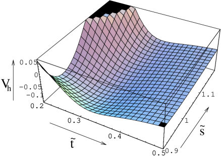
Figure 1: 3D plot of $V_{h}$ vs moduli $\tilde{s}$ $\&$ $\tilde{t}$ in units of $10^{12}~{}\rm GeV^{4}$ for parameter values $A=-1.60,W_{0}=1.7,a=0.1,k=0.1,\alpha=0.72,\alpha_{1}=1.5$. Here $A$ and $W_{0}$ represent values in the unit of $\Lambda_{N}^{3}$.

While $\alpha$ and $\alpha_{1}$ are chosen so as to have the AdS minimum, the constant parameter $k$ is set at $O(1)$ values to satisfy the condition (LABEL:const3). All the soft susy breaking parameters are now estimated assuming $k_{1}\sim 10^{-17}$ and $m\sim 10^{14}~{}\rm GeV$ along with Kähler correction as given via Eq.31. Then the gravitino mass given by (26) becomes,

$$m_{3/2}^{2}=\frac{1}{M_{p}^{4}}e^{-\frac{\alpha}{2\tilde{t}_{0}}-4\alpha_{1}{{\tilde{t}}^{2}}_{0}}~{}\frac{m^{6}}{16\tilde{s}_{0}\tilde{t}_{0}^{3}}\left[\frac{1}{(1+\sqrt{3})}~{}2\tilde{s}_{0}(\frac{k}{\tilde{s}_{0}}+2\frac{\ln{\tilde{s}_{0}}}{\tilde{s}_{0}})\right]^{2}.$$ (36)

In (36), the derivative $f^{\prime}(\tilde{s}_{0})\simeq(\frac{k}{\tilde{s}_{0}}+2\frac{\ln{\tilde{s}_{0}}}{\tilde{s}_{0}})$ have been used ignoring terms with $k_{1}\sim 10^{-17}$. The soft scalar mass (27) can be recast as,

$$\begin{split}m_{\alpha}^{2}=~{}&m_{3/2}^{2}+\frac{1}{M_{p}^{4}}\frac{e^{-\frac{\alpha}{2\tilde{t}_{0}}-4\alpha_{1}{{\tilde{t}}^{2}}_{0}}}{16\tilde{s}_{0}\tilde{t}_{0}^{3}}\frac{m^{6}}{\left(\frac{3}{4\tilde{t}_{0}^{2}}-\frac{\alpha}{4\tilde{t}_{0}^{3}}-2\alpha_{1}\right)}\\ &\left[((\ln{\tilde{s}_{0}})^{2}+k\ln{\tilde{s}_{0}}+k_{1}\tilde{s}_{0})\left(\frac{3}{2\tilde{t}_{0}}-\frac{\alpha}{4\tilde{t}_{0}^{2}}+4\alpha_{1}\tilde{t}_{0}\right)\right]^{2}\left[1-\frac{1}{4\tilde{t}_{0}^{2}}\frac{1}{\left(\frac{3}{4\tilde{t}_{0}^{2}}-\frac{\alpha}{4\tilde{t}_{0}^{3}}-2\alpha_{1}\right)}\right].\end{split}$$ (37)

The trilinear and bilinear couplings can now be calculated as before. The leading contributions to the trilinear coupling (29) and bilinear couplings (30) come from the gravitino mass $m_{3/2}$, which can be estimated from (36).

It is worthwhile is see that whether such a scenario could actually predict a global minimum with $\tilde{s}_{0}=1$. To investigate that, we illustrate our result with a $3D$-plot (fig 1) of the hidden sector scalar potential. It clearly exhibits the existence of a global AdS minimum of the potential which is essential for its stability. It can be seen that the resulting cosmological constant has been very finely tuned to make it compatible with the near Minkowskian but de- Sitter nature of the space-time of the present day universe. It is however worth pointing out here that the existence of the global minimum is extremely sensitive to the values of the parameters $\alpha,\alpha_{1},A,{W}_{0},a,k$ and $k_{1}$, thus rendering the model as fine tuned.

6 Discussions

String theory admits of numerous vacua, but only a very few of them are compatible with phenomenologically viable models in the low energy limit. It is therefore worthwhile to investigate the possible features of string inspired supergravity models from both particle phenomenology as well as cosmological point of view. This work is an attempt to establish the required constraints on the structures of these models in order to get the desired features. In this work we have considered a general supergravity scenario which simultaneously may address the issues of early inflationary phase of the universe, smallness of the observed cosmological constant in the present epoch as well as the TeV scale supersymmetry breaking which are known to be deeply connected to each other. In our analysis we assume the existence of a hidden sector with appropriate VEV of the moduli fields which couples gravitationally with the observable sector.Considering a dual scenario namely flux compactification and gaugino condensation at two different scales, we achieve to bring out the necessary constraints on the Kahler potential and superpotential so that the desired phenomenological values of the observable sector parameters can be obtained with no flat direction in the resulting scalar sector.We have shown that at least two hidden sector fields are necessary to achieve this.

We conclude by presenting a simple model in support of the analysis carried out in this work to illustrate that all the generic constraints on the Kähler and superpotential may be mutually compatible. Various parameters of the observable sector are estimated for this model. Our constraints thus put a set of restrictions on the class of supergravity models which they have to satisfy to yield phenomenologically viable results so that the following features can be achieved concomitantly :

• Soft supersymmetry breaking parameters are generated in the observable sector at the TeV scale.

• All the flat directions in the hidden sector are removed to have well-defined estimates of the soft breaking parameters.

• The resulting vacuum energy appearing from various mechanisms add up to a tiny positive value consistent with the presently observed de-Sitter character of the Universe.

7 Acknowledgment

DD thanks P2I, CNRS for the support received as a post-doctoral fellow. The authors would like to thank Pradipta Ghosh , Koushik Ray and Sourov Roy of the Department of Theoretical Physics, IACS, Kolkata, for fruitful discussions and suggestions.

References

- [1] H. P. Nilles, Phys. Rept. 110, 1 (1984).
- [2] D. Z. Freedman, P. van Nieuwenhuizen and S. Ferrara, Phys. Rev. D 13, 3214 (1976); S. Deser and B. Zumino, Phys. Lett. B 62, 335 (1976).
- [3] P. Nath, R. Arnowitt and A.H. Chamseddine, Trieste Lectures, 1983(World Scientific, Singapore,1984); E. Cremmer, S. Ferrara, L. Girardello and A. Van Proeyen, Nucl. Phys. B 212, 413 (1983); J. Bagger and E. Witten, Phys. Lett. B 118, 103 (1982).
- [4] S. K. Soni and H. A. Weldon, Phys. Lett. B 126, 215 (1983); V. S. Kaplunovsky and J. Louis, Phys. Lett. B 306, 269 (1993)
- [5] A. Brignole, L. E. Ibanez and C. Munoz, Nucl. Phys. B 422, 125 (1994) [Erratum-ibid. B 436, 747 (1995)]; arXiv:hep-ph/9707209.
- [6] R. Barbieri, S. Ferrara, D. V. Nanopoulos, K.S. Stelle, Phys.Lett.B113:219,1982.
- [7] Emilian Dudas, Phys.Lett.B 416, 309-318 (1998),
- [8] Y. Aghababaie, C.P. Burgess, S.L. Parameswaran, F. Quevedo, JHEP 0303:032,2003,
- [9] A. H. Chamseddine, R. Arnowitt and P. Nath, Phys. Rev. Lett. 49, 970 (1982); R. Barbieri, S. Ferrara and C. A. Savoy, Phys. Lett. B 119, 343 (1982); L. J. Hall, J. Lykken and S. Weinberg, Phys. Rev. D 27, 2359 (1983); P. Nath, R. Arnowitt and A. H. Chamseddine, Nucl. Phys. B 227, 121 (1983); N. Ohta, Prog. Theor. Phys. 70, 542 (1983)
- [10] Luis Alvarez-Gaume, J. Polchinski, Mark B. Wise, Nucl.Phys.B 221, 495 (1983).
- [11] E. Komatsu et al. [WMAP Collaboration], Five-Year Wilkinson Microwave Anisotropy Probe (WMAP) Observations:Cosmological Interpretation, Astrophys. J. Suppl. 180, 330 (2009) [arXiv:0803.0547 [astro-ph]].
- [12] A.Guth, Phys.Rev.D 23, 347 (1981)
- [13] A. B. Lahanas and D. V. Nanopoulos, Phys. Rept. 145, 1 (1987).
- [14] K. Inoue, M. Kawasaki, M. Yamaguchi and T. Yanagida, Phys. Rev. D 45, 328 (1992); S. Kelley, J. L. Lopez, D. V. Nanopoulos, H. Pois and K. j. Yuan, Phys. Lett. B 273, 423 (1991); M. Drees and M. M. Nojiri, Phys. Rev. D 45, 2482 (1992); S. Komine and M. Yamaguchi, Phys. Rev. D 63, 035005 (2001); J. R. Ellis, D. V. Nanopoulos and K. A. Olive,Phys. Lett. B 525, 308 (2002) J. Ellis, A. Mustafayev and K. A. Olive, arXiv:1004.5399 [hep-ph].
- [15] Shamit Kachru, Renata Kallosh, Andrei D. Linde, Sandip P. Trivedi, Phys.Rev.D68:046005, 2003
- [16] J. Maldacena and C. Nunez, Int. J. Mod. Phys. A16, 822 (2001), [arXiv:hep-th/0007018]; G.W. Gibbons, “Aspects of Supergravity Theories”, in Supersymmetry, Supergravity and Related Topics, eds. F. del Aguila, J.A. de Azcarraga and L.E. Ibanez, (World Scientific 1985) pp.346-351; B. de Wit, D.J. Smit and N.D. Hari Dass, Nucl. Phys. B283, 165 (1987).
- [17] Kiwoon Choi, Adam Falkowski, Hans Peter Nilles, Marek Olechowski, Nucl.Phys.B718:113-133,2005.
- [18] E. Dudas and S. K. Vempati,Nucl. Phys. B 727, 139 (2005)
- [19] Leonard Susskind, Carr, Bernard (ed.): Universe or multiverse, 247-266, e-Print: hep-th/0302219.
- [20] Shamit Kachru, Renata Kallosh, Andrei D. Linde, Juan Martin Maldacena, Liam P. McAllister, Sandip P. Trivedi, JCAP 0310:013,2003,
- [21] Edmund J. Copeland, M. Sami, Shinji Tsujikawa, Int.J.Mod.Phys.D15:1753-1936, 2006,
- [22] Michael R. Douglas, Shamit Kachru, Rev.Mod.Phys.79:733-796, 2007.
- [23] Ralph Blumenhagen, Mirjam Cvetic, Paul Langacker, Gary Shiu, Ann.Rev.Nucl.Part.Sci.55:71-139, 2005,
- [24] C.P. Burgess, R. Kallosh, F. Quevedo, JHEP 0310:056, 2003,
- [25] Michael R. Douglas, JHEP 0305:046, 2003,
- [26] Riccardo Argurio, Matteo Bertolini, Sebastian Franco, Shamit Kachru, JHEP 0706:017, 2007,
- [27] Adam Falkowski, Oleg Lebedev, Yann Mambrini, JHEP 0511:034, 2005 ; E. Dudas, Y. Mambrini, JHEP 0610:044,2006 ; O. Lebedev, V. Lowen, Y. Mambrini, H. P. Nilles and M. Ratz, JHEP 0702, 063 (2007); E. Dudas, Y. Mambrini, S. Pokorski, A. Romagnoni, JHEP 0804:015,2008,
- [28] Motoi Endo, Masahiro Yamaguchi, Koichi Yoshioka, Phys.Rev.D72:015004,2005.
- [29] Scott Watson, e-Print: arXiv:0912.3003 [hep-th]; Bobby Samir Acharya,Gordon Kane, Scott Watson, Piyush Kumar, Phys.Rev.D80:083529,2009.
- [30] Aalok Misra, Pramod Shukla, Nucl.Phys.B799:165-198,2008.
- [31] Nima Arkani-Hamed, Savas Dimopoulos, JHEP 0506:073, 2005.
- [32] U. Ellwanger, Phys. Lett. B 349, 57 (1995)