Continuous Markovian model for Lévy random walks
with superdiffusive and superballistic regimes

Abstract

We consider a previously devised model describing Lévy random walks (Phys. Rev E 79, 011110; 80, 031148, (2009)). It is demonstrated numerically that the given model describes Lévy random walks with superdiffusive, ballistic, as well as superballistic dynamics. Previously only the superdiffusive regime has been analyzed. In this model the walker velocity is governed by a nonlinear Langevin equation. Analyzing the crossover from small to large time scales we find the time scales on which the velocity correlations decay and the walker motion essentially exhibits Lévy statistics. Our analysis is based on the analysis of the geometric means of walker displacements and allows us to tackle probability density functions with power-law tails and, correspondingly, divergent moments.

1 Introduction

The Lévy-type behavior of anomalous Brownian motion has been found in a large variety of systems in nature (see, e.g., Mandl ; BG ; Biol1 ; Zasl1 ; Klaft1 ). It is characterized by the scaling law $|\delta\mathbf{r}|\propto t^{\beta}$ of the particle displacement $|\delta\mathbf{r}|$ during the time interval $t$ with an exponent $\beta>1/2$. The cases of $1/2<\beta<1$ and $\beta>1$ are usually referred to as the superdiffusive and superballistic regimes of the Lévy-type dynamics, respectively.

The continuous time random walk model, including its decoupled and coupled implementations, is now a widely used approach to describe Lévy-type stochastic processes (see, Klaft1 ; CTRW2 and references therein). Within the classical formulation Lévy flights are modeled as a sequence of random independent steps whose lengths are distributed according to a power-law probability density with diverging moments. Unfortunately, this model does not generate continuous trajectories. Indeed, by one step a Lévy walker can make a very long jump and such events in spite of being rather rare contribute substantially to the walker displacements. This feature is responsible for considerable problems met in describing Lévy-type processes in heterogeneous media and systems with boundaries. The coupled continuous time random walks CTRW2 , also referred to as Lévy random walks, do admit a representation of the walker motion in terms of continuous trajectories; this model just mimics the stochastic process at hand as a sequence of random independent steps whose length and duration are, in turn, random variables. The latter enables one to introduce a finite velocity of the walker motion during one step by connecting its initial and terminal points with a straight line and considering the walker motion along it uniform. Unfortunately, the resulting stochastic process looses the Markov property in the strict sense.

There have been several attempts to develop a description of Lévy-type random walks starting from a certain Markovian continuous process with, may be, nonlinear (multiplicative) Langevin forces. In particular, it is a description of the decoupled continuous time random walks based on the corresponding Langevin equation Fogedby , the combination of a conventional stochastic process governed by a linear Langevin equation with additive noise where, however, time itself is a random nondecreasing variable HN , models bases on stochastic differential equations with non-Gaussian Lévy white noise NGLN1 ; NGLN2 , and the semiclassical Fokker-Planck equation describing quantum interaction of atoms with laser beams F1 ; F2 , as well as models using the Boltzmann equation with scattering characterized by power-law distribution Fr1 ; Fr2 ; Fr3 . There is also an approach to describe anomalous diffusion based on the nonlinear Fokker-Planck equation derived using the generalized entropy Tsalis .

In systems far from thermodynamics equilibrium and complex systems nonlinear stochastic processes are widely met and have been studied in connection with the appearance of power-law distributions and long-time tails of time correlation functions (see, e.g., K1 ; K2 as well as K3 ; KW and references therein).

The generalized Cauchy stochastic process, which is governed by the following Langevin equation with additive and multiplicative noise KW

$$\tau\frac{dv}{dt}=-[\lambda+\sqrt{2\tau}\xi_{m}(t)]*v+\sqrt{2\tau}v_{a}\xi_{a}(t)$$ (1a)

has been employed to study stochastic behavior of various nonequilibrium systems, in particular, lasers K1 , on-off intermittency Nak5 , economic activity Nak9 , passive scalar field advected by fluid Nak11 , etc. Here $$v \tau \lambda \xi_{m}(t) \xi_{a}(t) v_{a} \sqrt{2} \xi(t) v$$ is a certain random variable, is a characteristic “microscopic” time scale of its dynamics, is a friction constant, and are independent components of white noise of unit amplitude, the parameter quantifies the intensity of additive noise, and the asterisk indicates that equation (1a) is written in the Hänggi-Klimontovich form. The coefficients are introduced into (1a) for the sake of convenience. Equation (1a) is equivalent to the following Langevin equation with a single white noise source and the amplitude depending nonlinearly on the random variable KW

$$\tau\frac{dv}{dt}=-\lambda v+\sqrt{2\tau\big{(}v_{a}^{2}+v^{2}\big{)}}\xi(t)$$ (1b)

because both of them are described by the same Fokker-Planck equation for the probability density $P(v,t)$

$$\tau\frac{\partial P}{\partial t}=\frac{\partial}{\partial v}\left[\big{(}v_{a}^{2}+v^{2}\big{)}\frac{\partial P}{\partial v}+\lambda vP\right]\,.$$ (2)

Appealing to qualitative arguments and a numerical example Sakaguchi Saka demonstrated that the generalized Cauchy process (1a) can give rise to Lévy flights in the space $x$ on time scales $t\gg\tau$ if the random variable $v$ is regarded as the velocity $v=dx/dt$ of a Brownian particle.

Previously we1 ; we2 we analyzed in detail such random walks governed by the Langevin equation (1b) when the induced Lévy-type process is superdiffusive. In particular, it has been demonstrated we1 that on time scales $t\gg\tau$, related with the crossover to Lévy-type behavior, the scaling law $\delta x\propto t^{\beta}$ with the exponent $1/2<\beta<1$ is due to the impact of extremely large fluctuations in the velocity pattern $\{v(t)\}$. Roughly speaking, the peak velocity $\{v_{\text{max}}(t)\}$ times the duration $\tau$, where $v_{\text{max}}$ is the maximal value of the velocity attained during the time interval $t$, is the main contribution to the particle displacement $\delta x(t)$. As a consequence, the estimate $\delta x\sim v_{\text{max}}\tau$ holds and the characteristic scaling law is related to the statistics of the occurrence of extreme fluctuations in the observation interval $t$.

It should be noted that the constructed random process neither belongs to the decoupled nor to coupled continuous time random walks. Indeed, on one hand side, this Brownian particle moves continuously and, on the other hand, its motion with the “elementary” time fragment $t$ is not uniform but extremely heterogeneous. The latter is actually the mechanism preserving the Markov property of such random walks. Naturally on time scales about $\tau$ and the corresponding spatial scales $\ell=v_{a}\tau$ random walks governed by the Langevin equation (1b) are ballistic, $\delta x(t)\propto t$, because of the strong velocity correlations on such scales. In our paper we2 we have developed a special singular perturbation technique and proved, for the superdiffusive regime, that the stochastic process (1b) indeed describes the Lévy-type random walks on time scales $t\gg\tau$. At the critical value $\lambda_{c}$ separating the superdiffusive and superballistic regimes the constructed perturbation technique exhibits some singularities at intermediate steps, but the final results turn out to be free from any singularity at $\lambda=\lambda_{c}$. This problem seems to be related to the well-known conflict with dynamics in constructing the superballistic Lévy flights, extensively discussed in the review Zasl2 .

The purpose of the present paper is, first, to demonstrate that the developed model we1 ; we2 not only describes the superdiffusive Lévy-type random walks but also superballistic ones. A second aim is to analyze the crossover between the time scales $t\sim\tau$ and $t\gg\tau$ in the behavior of the walker displacements. The latter result will clarify the behaviour at the time scales for which velocity correlations become insignificant and Lévy-type dynamics arises.

It should be noted that superballistic transport is expected to arise in such systems as atmospheric turbulence sb1 ; sb2 , two-dimensional turbulence sb3 , a collisionless plasma driven in magnetic field reversal with an electric field in the presence of magnetic turbulence sb4 . It also has been observed experimentally in a fully developed turbulent laboratory water flow sb5 as well as in a one-dimensional expansion of cold atomic clouds in a magneto-optical trap under the impact of laser beams sb6 . In spite of these objects, strictly speaking, do not belong to the systems under consideration, it was found that the notion of Lévy-type random walks sb2 ; sb3 or stochastic differential equations sb6 gives rise to the adequate description of these superballistic phenomena. Large-scale animal movements in searching resource patches, mates, etc. or dispersal also exhibit the Lévy-type pattern (for a review see For1 ; For2 ; Fog3 ) and there are conditions when the optimal random search becomes of the ballistic type as a limit case of Lévy-type motion Fog4 ; Fog5 . Lévy type behavior is relevant to stock indices, too, and the indices matching the superballistic Lévy flights were found, in particular, for the Brazil BVSP index and the Argentine MERV index EPh1 , for foreign exchange rate in Brazil and South Korea EPh2a ; EPh2b , and the absolute value of the returns in the Indian market indices EPh3

2 Model

Let us restrict our consideration to a dimensionless description of the stochastic processes at hand and, thereby, measure time in units of $\tau$, i.e. $t\to\tau t$ and spatial variables in units of $\ell$, i.e. $x_{i}\to\ell x_{i}$. In these units the continuous Markovian random walks under consideration are governed by the following equations

$$\frac{dx_{i}}{dt} =v_{i}\,,$$ (3)

$$\frac{dv_{i}}{dt} =-\left(n+\alpha\right)v_{i}+\sqrt{2(1+\mathbf{v}^{2})}*\xi_{i}(t)\,.$$ (4)

Here $\mathbf{r}=\{x_{1},\dots,x_{n}\}$ is the current position of a random walker in the Euclidean $n$-dimensional space $\mathbb{R}^{n}$ and $\mathbf{v}=\{v_{1},\dots,v_{n}\}$ is the velocity of its motion in this phase space, $\{\xi_{1}(t),\ldots\xi_{n}(t)\}$ is the collection of mutually independent components of Gaussian white noise,

$$\left<\xi_{i}(t)\right>=0\,,\quad\text{and}\quad\left<\xi_{i}(t)\xi_{i^{\prime}}(t^{\prime})\right>=\delta_{ii^{\prime}}\delta(t-t^{\prime})\,,$$ (5)

and, as before, the asterisk indicates that equation (4) is written in the Hänggi-Klimontovich form. The parameter $\alpha$ is assumed to be taken from the interval

$$0<\alpha<2\,.$$ (6)

Previously we2 dealing with this model for $1<\alpha<2$ we demonstrated that in the limit $t\gg 1$ the characteristic amplitude $|\delta\mathbf{r}|$ of the walker displacements scales with time $t$ as $|\delta\mathbf{r}(t)|\propto t^{1/\alpha}$, matching the superdiffusive Lévy random walks. Besides, the probability density $P(\mathbf{\delta r},t)$ of the walker displacement $\delta\mathbf{r}\in\mathbb{R}^{n}$ is found to possess the required asymptotics $P(\mathbf{\delta r},t)\propto|\delta\mathbf{r}|^{-(n+\alpha)}$ when $|\delta\mathbf{r}|\to\infty$. These expressions stem directly from the obtained dependence of the generating function for $t\gg 1$

$$G(\mathbf{k},t)=\left<e^{i\mathbf{kr}}\right>=\exp\left\{-\Lambda_{\text{min}}t|\mathbf{k}|^{\alpha}\right\},$$ (7)

where $\Lambda_{\text{min}}>0$ is the minimal eigenvalue of the corresponding Fokker-Planck equation. In the 1D-case it is given by the expression

$$\Lambda_{\text{min}}=\frac{\Gamma\left(\dfrac{2-\alpha}{2}\right)}{2^{\alpha-1}\Gamma\left(\dfrac{\alpha}{2}\right)\Gamma\left(\alpha\right)}\,,$$ (8)

where $\Gamma(\dots)$ is the gamma function.

As noted before all these final results do not exhibit singularities when $\alpha\to 1$ whereas the constructed perturbation technique does at its intermediate steps. This feature poses a question as to whether the stated model (3), (4) does describe the Lévy random walks in a wider region of parameters including the whole interval (6) and comprising superdiffusive as well as superballistic dynamics.

In the next section this hypothesis will be justified numerically; here, we present some heuristic arguments for the absence of any singularity in the behavior of the given system when the parameter $\alpha$ is taken from the interval $0<\alpha\leq 1$.

Canonical form of equation (4)

Dealing with the one dimensional stochastic processes governed by the Langevin equation (4) for $n=1$ let us make use of the nonlinear transformation KW

$$v=\sinh(u)$$ (9)

reducing equation (4) to the following Langevin equation with additive noise

$$\frac{du}{dt}=-\alpha\tanh(u)+\sqrt{2}\xi(t)\,.$$ (10)

In obtaining expression (10) we, first, converted equation (4) into the Stratonovich form and only then performed the transformation (9). According to Konno and Watanabe KW expression (10) can be regarded as the canonical form of such stochastic differential equations with multiplicative noise.

From the Fokker-Planck equation

$$\frac{\partial P}{\partial t}=\frac{\partial}{\partial u}\left[\frac{\partial P}{\partial u}+\alpha\tanh(u)P\right]$$

corresponding to the Langevin equation (10) we obtain the steady state distribution of the random variable $u$

$$P_{c}(u)=\frac{A_{c}}{[\cosh(u)]^{\alpha}}\,,$$ (11)

where $A_{c}$ is the normalization constant. In particular, for $\alpha\sim 1$ the constant $A_{c}\sim 1$ too and for $\alpha\ll 1$ the estimate $A_{c}=\alpha/2$ holds. From the Langevin equation (10) we can estimate the time scale $T_{c}$ characterizing the formation of the steady state distribution (11) as $T_{c}\sim 1$ for $\alpha\sim 1$ and $T_{c}\sim 1/\alpha^{2}$ for $\alpha\ll 1$.

We conclude that the statistical properties of the random variable $u$ cannot exhibit any singularity for the parameter $\alpha$ lying inside the interval under consideration, i.e. $\alpha\in(0,2)$. The parameter $\alpha$ just affects the weight of extreme fluctuations with respect to their contribution to the walker displacement, changing the exponent of its time dependence. Moreover, in studying these extreme fluctuations we can approximate the function $\tanh(u)$ by the signum function $\text{sign}(x)$, i.e., make use of the replacement $\tanh(u)\to\text{sign}(x)$ and perform the transformations $u\to u/\alpha$ and $t\to t/\alpha^{2}$. This reduces equation (10) to the following equation

$$\frac{du}{dt}=-\text{sign}(u)+\sqrt{2}\xi(t)\,.$$ (12)

In deriving this equation the white noise transformation $\xi(t)\to\alpha\xi(t)$ caused by the given time renormalization and stemming from the induced transformation of the correlation function

$$\left<\xi(t)\xi(t^{\prime})\right>=\delta(t-t^{\prime})\underset{t\to t/\alpha^{2}}{\longrightarrow}\alpha^{2}\delta(t-t^{\prime})$$

has been taken into account. Equation (12) does not contain any parameter, which seems to be the reason for the universal behavior of such systems.

Therefore, it is quite natural to expect that for $0<\alpha\leq 1$ model (3), (4) also describes the Lévy-type random walks with, maybe, the superballistic dynamics provided the expression $\delta x(t)\propto t^{1/\alpha}$ holds. The singularities arising at intermediate steps of the perturbation technique seem to be caused by anomalous behavior of integrals similar to

$$\int\limits_{-\infty}^{\infty}P(x,t)\sin(kx)\,dx\propto\int\limits_{-\infty}^{\infty}\frac{\sin(kx)}{|x|^{1+\alpha}}\,dx$$

as $k\to 0$. For $\alpha<1$ this integral also leads to nonanalytic dependencies on the wave number $k$ and must vanish for the symmetry reasons only.

3 Numerical results

In order to justify the fact that the model (3), (4) does describe the Lévy-type random walks on time scales $t\gg 1$ for $0<\alpha<2$ the system of equations (3), (4) has been solved numerically. Then the obtained results were used to calculate the geometric mean value

$$\ln\!\big{[}\overline{r}_{g}(t)\big{]}=\left<\ln\!\big{(}|\delta\mathbf{r}|\big{)}\right>$$ (13)

of the walker’s displacement $\delta\mathbf{r}$ during the time interval $t$ as well as the probability density function $P(|\delta\mathbf{r}|,t)$. It should be pointed out that logarithmic mean values similar to (13) form a rather efficient tool for analyzing statistical data with power-law distributions possessing diverging moments KW . It is due to the geometric mean converging for any power-law distribution that can be normalized to unity and, thus, enables us to analyze superdiffusive and superballistic regimes with any possible value of the exponent $\alpha\in(0,2)$ using the same quantities. The geometric mean value introduced via expression (13) can be also treated as the limit case of constructing the Hurst exponent $H(\varepsilon)$

$$\left<|\delta\mathbf{r}|^{\varepsilon}\right>^{1/\varepsilon}\propto t^{H(\epsilon)}\quad\text{for}\quad\varepsilon\to+0\,.$$

In addition, when the random variables $\delta\mathbf{r}(t)$ are characterized by an autonomous probability density $\mathcal{P}\left(|\delta\mathbf{r}|/t^{\beta}\right)$ expression (13) reads

$$\ln\!\big{[}\overline{r}_{g}(t)\big{]}=\int\limits_{0}^{\infty}\ln(\zeta)\mathcal{P}(\zeta)d\zeta+\beta\ln(t)\,,$$

which allows us to separate the time dependence of the scaling low $|\delta\mathbf{r}(t)|\propto t^{\beta}$ from the corresponding numerical coefficients.

If the generating function $G(\mathbf{k},t)$ for the quantities $\{\delta\mathbf{r}\}_{t}$ is given by expression (7) formula (13) yields

$$\overline{r}_{g}(t)=\Lambda_{g}\cdot t^{1/\alpha},$$ (14)

as shown in Appendix A. In particular, we obtain in the 1D-case the coefficient

$$\Lambda_{g}|_{n=1} =\Lambda_{\text{min}}^{1/\alpha}\cdot\exp\left\{\gamma\,\frac{(1-\alpha)}{\alpha}\right\},$$ (15)

and for the 2D-case

$$\Lambda_{g}|_{n=2} =2\Lambda_{\text{min}}^{1/\alpha}\cdot\exp\left\{\gamma\,\frac{(1-\alpha)}{\alpha}\right\}.$$ (16)

Here $\gamma\approx 0.5772$ is the Euler-Mascheroni constant.

If the random variable $\delta\mathbf{r}$ obeys the Lévy statistics, then the asymptotics of the probability density $P(|\delta\mathbf{r}|,t)$ is also determined by equation (7) for the generating function $G(\mathbf{k},t)$. Moreover, provided the walker displacement $\delta\mathbf{r}$ is measured in units of the corresponding geometric mean $\overline{r}_{g}(t)$, i.e. in terms of $\rho=|\delta\mathbf{r}|/\overline{r}_{g}(t)$, its probability density is characterized by the asymptotics (Appendix B)

$$\mathcal{P}(\rho)=\frac{\varpi_{\rho}}{\rho^{1+\alpha}}\qquad\text{as}\quad\rho\to\infty\,,$$ (17)

where in the 1D-case the coefficient reads

$$\varpi_{\alpha}|_{n=1} =\frac{2}{\pi}\sin\left(\frac{\pi\alpha}{2}\right)\Gamma\left(1+\alpha\right)e^{\gamma(\alpha-1)}$$ (18)

whereas in the 2D-case

$$\varpi_{\alpha}|_{n=2} =\frac{2}{\pi}\sin\left(\frac{\pi\alpha}{2}\right)\left[\Gamma\left(1+\frac{\alpha}{2}\right)\right]^{2}e^{\gamma(\alpha-1)}\,.$$ (19)

Expressions (14) and (17) are the key results for the numerical verification of the Lévy-type dynamics of the random walks under consideration. Namely, analyzing the numerical simulation data it is possible to verify whether the constructed time dependence of the geometric mean $\overline{r}_{g}(t)$ and the probability density $P(\mathbf{r},t)$ actually do obey expressions (14) and (17).

Figure 1: The geometric mean of the walker displacements versus the observation time interval and the probability density of the walker displacements. In simulating 1D and 2D models the integration time steps was set equal to $dt=0.05$ and $dt=0.02$, respectively, the integration time was $T=10^{8}$. The other parameters are shown in the panels.

For the 1D-case the system of equations (3), (4) has been solved numerically employing the stochastic Runge-Kutta method SRI2W1 approximating one-dimensional Wiener process Itô equations with strong order (4.0,1.5) SRK1 . The time step $dt=0.05$ for integration yields results, which were stable with respect to a decrease of $dt$. The integration time was $T=10^{8}$. For the 2D-case this system was solved using the stochastic Runge-Kutta method RI1 approximating multidimensional Wiener process Itô equations with weak order (3,2) SRK2 . The integration time step was chosen as $dt=0.02$ yielding stable results. The integration time was also $T=10^{8}$.

Figure 1 depicts the obtained results for the 1D and 2D models. The relevant analytic time dependence of the geometric mean $\overline{x}_{g}(t)$, in the 1D-case specified by expressions (8), (14), and (15), is also exhibited in Fig. 1. In particular, for $\alpha=1.5$, 1.0 and 0.5 we obtain $\Lambda_{g}\approx 1.46$, $1$, and $0.130$, respectively. As seen in Fig. 1 the corresponding analytic dependence fits the numerical data quite well if the time interval $t$ exceeds a value of about $t\sim 100$. For time scale $t\sim 1$ at which the velocity correlations should be significant and, consequently, the walker behaviour has to be ballistic, the effective exponent of the curve $\overline{x}_{g}(t)$ is about unity as expected. Thus, the constructed curves actually describe the crossover from the ballistic motion on time scales $t\sim 1$ to the superdiffusive or superballistic regimes of the Lévy-type random walks for $t\gtrsim 100$ for all the analyzed values of the parameter $\alpha$. In the 2D-case an analytic expression for the minimal eigenvalue $\Lambda_{\text{min}}$ is not known. Therefore, we can compare only the slope of curves (in log-log scale) evaluated numerically and the corresponding exponents of the theoretical dependence (14). As seen in Fig. 1 these values again fit each other when $t\gtrsim 100$ for the parameter $\alpha\leq 1$ as well as $\alpha>1$.

The numerical data for the probability density also exhibit the desired asymptotics for both the 1D- and 2D-cases. According to expression (18) in the 1D-case the coefficient $\varpi_{\rho}$ takes the values $\varpi_{\rho}\approx 0.799$, 0.300 for $\alpha=1.5$, 0.5, respectively, and $\varpi_{\rho}=2/\pi$ for $\alpha=1$. For the 2D-case, by virtue of (19), it is 0.507, 0.277 and 1/2, respectively. The corresponding theoretical asymptotics of the probability density $\mathcal{P}(\rho)$ are also shown in Fig. 1. In particular, as seen in this figure the function $\mathcal{P}(\rho)$ tends to asymptotics (17) from above for $\alpha=1.5$.

For the parameter $\alpha=1.5$ the accuracy between the analytical and numerical results is expected and can be regarded as a verification of the used implementation of the employed numerical algorithms. At the same time, for $\alpha=1.0$ and 0.5 it is this accuracy that justifies the Lévy-type behavior of the stochastic process governed by model (3), (4) for the parameter $\alpha$ lying in the interval $0<\alpha\leq 1$.

It is necessary to note that the similarity of the plots for the 1D and 2D-cases with respect to the corresponding exponents is a consequence of the fact that the friction coefficient $(\alpha+n)$ entering equation (4) depends on the space dimension $n$. So in the 2D-case the components $\xi_{1}(t)$ and $\xi_{2}(t)$ of white noise individually undergo stronger dissipation and only their interplay leads to the same scaling law of the particle displacement magnitudes $\{|\delta\mathbf{r}|_{t}\}$. The difference between the plots showing the time dependence of the geometric means $\overline{x}_{g}(t)$ and $\overline{r}_{g}(t)$ for $\alpha=1$ enables us to claim that the ballistic-like behavior of the geometric mean on time scales $t\lesssim 1$ and its ballistic regime for $\alpha=1$ must be characterized by the same exponent but not the numerical cofactors. So their visible equality in the 1D-case seems to be just coincidental. It also should be noted that in the 2D-case the probability density $\mathcal{P}(\rho)$ attains its maximum at a certain point $\rho_{\text{max}}>0$, whereas in the 1D-case this maximum is located at the origin $\rho=0$. In fact, even in the 2D-case the probability density $P(\delta\mathbf{r},t)=P(|\delta\mathbf{r}|,t)$ of the random vector $\delta\mathbf{r}$ gets its maximum at the origin too. However, the depicted probability density $\mathcal{P}(\rho)$ is proportional to the function $P(|\delta\mathbf{r}|,t)$ with a coefficient depending on $|\delta\mathbf{r}|$, namely, $\mathcal{P}(\rho)\propto|\delta\mathbf{r}|P(|\delta\mathbf{r}|,t)$, which causes the shift of its maximum from the origin.

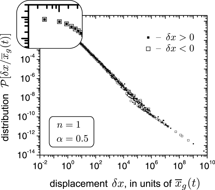
Figure 2: The two side probability density of the walker displacements. The data for the 1D-model with the parameter $\alpha=0.5$ matching the superballistic regime are presented. The integration step was set equal to $dt=0.05$ and the integration time was $T=10^{8}$.

Finalizing the present section let us discuss ergodic properties of the investigated stochastic process. Ergodicity usually means that the ensemble average

$$\left<A\right>:=\int AP(A)dA\,,$$

where $P(A)$ is the probability density, and the time average

$$\overline{A}:=\frac{1}{t}\int\limits_{0}^{t}A(t^{\prime})dt^{\prime}$$

of an observable $A$ are equal in the infinite-time limit $t\to\infty$. The condition

$$\left<\left(\overline{A}-\left<A\right>\right)^{2}\right>\to 0\quad\text{as}\quad t\to\infty$$

is widely used as a criterion for this equality erg1 . A system obeying this criterion is said to be ergodic in the mean square sense. Therefore, the notion of ergodicity also includes the measure of convergence. This type of ergodicity can be broken when the parameter $A$ is distributed with a probability density possessing power-law tails which cause the divergence of its moments F2 ; erg2 ; erg3 . Moreover, studying the ergodicity one may focus not on a single trajectory of the system motion as a whole but treat it as a collection of various fragments. As a result, a system could be regarded as ergodic with respect to one variable and loose the ergodicity according to the properties of another variable. Such a partial ergodicity is met in the system at hand. In fact, each of the plots in Fig. 1 has been built using numerical data generated during the system motion along a single sufficiently long trajectory. So the system ergodicity with respect to quantities such as the geometric mean of walker displacements and their distribution function is justified by the accuracy between the presented numerical data and the theoretical results related to the corresponding ensemble averages. As illustrative example, Figure 2 depicts the two-sided probability density $P(\delta x,t)$ of one-dimensional random walks for the parameter $\alpha=0.5$, i.e. for the superballistic regime. This probability density, in contrast to the preceding constructions, takes into account also the direction of the walker displacements. As seen in this figure even in the case of the superballistic regime the probability density of the walker displacements constructed by averaging over time is highly symmetric. In contrast, under the same conditions such ergodicity does not hold with respect to any quantity depending on the sign of the walker position at the $x$-axis. Indeed, the mean time $t_{a}$ spent by the random walker inside a small neighborhood $\mathbb{Q}_{a}$ of its initial point $x_{0}=0$ whose size is about $a$ can be estimated as

$$t_{a}\sim\int\limits_{0}^{\infty}\frac{a}{\overline{x}_{g}(t)}\,dt\,.$$ (20)

Estimate (20) stems directly from the expression for the walker residence time $t_{a}$ inside the domain $\mathbb{Q}_{a}$

$$t_{a}=\int\limits_{0}^{\infty}dt\int\limits_{\mathbb{Q}_{a}}dx\,\delta[x-x(t)]$$ (21)

for a given realization $\{x(t)\}$ of the walker trajectory and the estimate of the probability density of finding the walker at the initial point $x=0$

$$\mathcal{G}(0,t)=\left<\delta[x-x(t)]\right>|_{x=0}\sim\frac{1}{\overline{x}_{g}(t)}\,.$$

Integral (20) converges at the upper boundary for the parameter $\alpha<1$ since in this case the geometric mean $\overline{x}_{g}(t)\propto t^{1/\alpha}$ grows faster than $t$. As a result, there is a certain probability that the walker never returns to its initial point and, thus, the walker will practically spend all the time in the region $x>0$ or $x<0$ as $t\to\infty$. As the averages over ensemble are concerned, the properties of the given random walks should be symmetrical with respect to the reflection $x\mapsto-x$.

4 Conclusion

We have considered the stochastic process governed by equations (3), (4) and numerically demonstrated that on time scales $t\gg 1$ this process describes the Lévy-type random walks with the superballistic, ballistic, and superdiffusive dynamics, depending on the value of the parameter $\alpha$, namely, for $0<\alpha<1$, $\alpha=1$, and $1<\alpha<2$, respectively. In this way we have justified that the given model is a continuous Markovian implementation of the Lévy flights or the Lévy walks of all the main types that at the “microscopic” level admits the notion of continuous trajectories.

To analyze the statistical properties of stochastic processes for which the moments of the probability density can diverge the notion of geometric mean was used and the walker displacements were measured in units of the corresponding geometric means. This enabled us to compare the numerical data and theoretical results not only for one-dimensional systems but also for two-dimensional models exemplifying the validity of the models for the case of multi-dimensional random walks.

The analyzed crossover between the time scales $t\sim 1$ and $t\gg 1$ has shown that the Lévy-type behavior arises on scales $t\gtrsim 100$. On scales $t\sim 1$, where the velocity correlations are significant, the random walks are ballistic. The direct simulation of the system motion along individual sufficiently long trajectories has demonstrated the fact that the system at hand is partly ergodic, i.e. it is ergodic with respect to quantities such as the geometric mean of the walker displacements and their distribution, independently of whether the regime being superdiffusive or superballistic. In the latter case, however, there are quantities for which ergodicity is broken. At least the superballistic Lévy-type random walks described by the given model are only partly ergodic.

Appendix A Geometric mean and generating function

Let us consider a random vector $\mathbf{r}$ of the $n$-dimensional space $\mathbb{R}^{n}$ ($n=1,2,\ldots$) whose statistical properties are described by a given probability density $P(\mathbf{r})$. Using this function we, first, construct the generating function $G(\mathbf{k})$

$$G(\mathbf{k}):=\left<e^{i\mathbf{kr}}\right>=\int\limits_{\mathbb{R}^{n}}e^{i\mathbf{kr}}P(\mathbf{r})\,d\mathbf{r}\,,\quad\mathbf{k}\in\mathbb{R}^{n}$$ (22)

which is the Fourier transform of the probability density and, then, the function

$$G_{s}(\mathbf{k}):=\frac{1}{\Omega_{n,s}}\int\limits_{\mathbb{R}^{n}}\frac{G(\mathbf{k}^{\prime})}{|\mathbf{k}-\mathbf{k}^{\prime}|^{n-s}}\,d\mathbf{k}^{\prime}\,,$$ (23)

where the exponent $0<s<1$, the coefficient

$$\Omega_{n,s}=\pi^{\tfrac{n}{2}}\frac{2^{s}\Gamma\left(\dfrac{s}{2}\right)}{\Gamma\left(\dfrac{n-s}{2}\right)}$$ (24)

and, as before, $\Gamma(\ldots)$ is the gamma function. The substitution of (22) into (23) yields the equality

$$G_{s}(\mathbf{k})=\int\limits_{\mathbb{R}^{n}}e^{i\mathbf{kr}}P(\mathbf{r})\,d\mathbf{r}\left[\frac{1}{\Omega_{n,s}}\int\limits_{\mathbb{R}^{n}}\frac{e^{i\mathbf{qr}}}{|\mathbf{q}|^{n-s}}\,d\mathbf{q}\right]\,.$$ (25)

A direct calculation of the last integral leads us to the expression

$$G_{s}(\mathbf{k})=\int\limits_{\mathbb{R}^{n}}\frac{e^{i\mathbf{kr}}}{|\mathbf{r}|^{s}}P(\mathbf{r})\,d\mathbf{r}\,.$$ (26)

So, by definition, the mean value of the moment $1/|\mathbf{r}|^{s}$ is

$$\left<\frac{1}{|\mathbf{r}|^{s}}\right>:=\int\limits_{\mathbb{R}^{n}}\frac{P(\mathbf{r})}{|\mathbf{r}|^{s}}\,d\mathbf{r}=\frac{1}{\Omega_{n,s}}\int\limits_{\mathbb{R}^{n}}\frac{G(\mathbf{k})}{|\mathbf{k}|^{n-s}}\,d\mathbf{k}$$ (27)

by virtue of (23) and (26).

Let us introduce the symmetrized generating function $g(k)$ by integrating the generating function $G(\mathbf{k})$ over the $n$-dimensional sphere $\mathbb{S}_{n,k}=\{\mathbf{k}:|\mathbf{k}|=k\}$

$$g(k):=\frac{1}{S_{n}k^{n-1}}\oint\limits_{\mathbb{S}_{k}}G(\mathbf{k})\,d\sigma\,,$$ (28)

where $S_{n}k^{n-1}$ is the surface area of the sphere $\mathbb{S}_{n,k}$ and the coefficient

$$S_{n}=\frac{2\pi^{\tfrac{n}{2}}}{\Gamma\left(\dfrac{n}{2}\right)}\,.$$ (29)

In particular, for the random vector $\mathbf{r}$ with the spherically symmetric distribution density $P(r)$ and, thus, the spherically symmetric generating function $G(k)$ the identity $g(k)\equiv G(k)$ holds. In these terms expression (27) reads

$$\left<\frac{1}{|\mathbf{r}|^{s}}\right>=\frac{S_{n}}{\Omega_{n,s}}\int\limits_{0}^{\infty}k^{s-1}g(k)\,dk\\ {}=-\frac{S_{n}}{s\cdot\Omega_{n,s}}\int\limits_{0}^{\infty}k^{s}\frac{dg(k)}{dk}\,dk\,.$$ (30)

Then using the series

$$|\mathbf{r}|^{-s} =1-s\ln|\mathbf{r}|+O\left(s^{2}\right)\,,$$

$$k^{s} =1+s\ln k+O\left(s^{2}\right)\,,$$

$$2^{s} =1+s\ln 2+O\left(s^{2}\right)\,,$$

$$\Gamma\left(\frac{s}{2}\right) =\frac{1}{s}\left[1-\gamma\frac{s}{2}+O\left(s^{2}\right)\right]\,,$$

$$\Gamma\left(\frac{n-s}{2}\right) =\Gamma\left(\frac{n}{2}\right)\left[1-\Psi\!\left(\frac{n}{2}\right)\frac{s}{2}\right]+O(s^{2})$$

where, $\Psi(\ldots)$ is the digamma function and, as before, $\gamma\approx 0.5772$ is the Euler-Mascheroni constant, we expand the left and right sides of expression (30) into series of $s$ up to the first order in $s$. In this way for the geometric mean value $\overline{r}_{\text{g}}$ of the random vector $\mathbf{r}$ defined as

$$\ln\left[\overline{r}_{\text{g}}\right]:=\left<\ln|\mathbf{r}|\right>$$ (31)

we obtain the formula

$$\ln\left[\overline{r}_{\text{g}}\right]=\int\limits_{0}^{\infty}\ln(k)\,\frac{dg(k)}{dk}\,dk-\gamma+\frac{1}{2}\left[\Psi\!\left(\frac{n}{2}\right)-\Psi\!\left(\frac{1}{2}\right)\right]$$ (32)

relating the geometric mean value $\overline{r}_{\text{g}}$ and the generating function $G(\mathbf{k})$ via $g(k)$. In deriving expression (32) the equality

$$\Psi\left(\frac{1}{2}\right)=-\gamma-2\ln 2$$

has been also taken into account. In particular, in the 1D-case the last summand is absent and for the 2D-case where $\Psi(n/2)=\Psi(1)=-\gamma$ its value is $[\Psi(1)-\Psi(1/2)]/2=\ln 2$. It should be noted that expression (32) can be also regarded as a specific implementation of the Hadamard type fractional calculus (see, e.g., Kilbas ).

For the generating function $G(\mathbf{k})=\exp\left(-\omega|\mathbf{k}|^{\alpha}\right)$, where $\omega>0$ and $\alpha>0$ are some positive constants, expression (32) reads

$$\ln\overline{r}_{\text{g}}=\frac{1}{\alpha}\ln\omega+\gamma\frac{(1-\alpha)}{\alpha}+\frac{1}{2}\left[\Psi\!\left(\frac{n}{2}\right)-\Psi\!\left(\frac{1}{2}\right)\right].$$ (33)

In obtaining the latter formula we have taken into account the equality

$$\int\limits_{0}^{\infty}\ln(k)\,e^{-k}\,dk=-\gamma\,.$$

A similar expression can be obtained for the $n$-dimensional generalized Cauchy distribution KonoPrivate .

Formula (33) immediately leads us to the desired expression (14) for $\omega=\Lambda_{\text{min}}t$.

Appendix B Asymptotics of the probability density and generating function

As in Appendix A, let us consider a random vector $\mathbf{r}\in\mathbb{R}^{n}$ whose statistical properties are specified by a given distribution density $P(\mathbf{r})$. Now, however, some additional assumptions about it are adopted. Namely, the leading term in the asymptotic series of the probability density $P(\mathbf{r})$ as $\mathbf{r}\to\infty$ is considered to be a spherically symmetrical power-law function. In other words, the equality

$$P(\mathbf{r})=\frac{\varpi}{r^{n+\alpha}}+o\left(\frac{1}{r^{n+\alpha}}\right),$$ (34)

where $r=|\mathbf{r}|$ and the parameters $\varpi>0$ and $0<\alpha<2$ is presumed to hold. The inequality $0<\alpha<2$ imposed on the exponent $\alpha$ assures us of the required convergence of the integral

$$\int\limits_{\mathbb{R}^{n}}P(\mathbf{r})\,d\mathbf{r}=1$$

and meets the divergence of the second moment

$$\int\limits_{\mathbb{R}^{n}}\mathbf{r}^{2}P(\mathbf{r})\,d\mathbf{r}=\infty$$

being the characteristic feature of the systems at hand. The purpose of the present Appendix is to relate the given asymptotics of the probability density to corresponding asymptotics of the generating function $G(\mathbf{k})$ as $\mathbf{k}\to 0$.

By virtue of (22) and (34) we have

$$1-G(\mathbf{k})=\int\limits_{\mathbb{R}^{n}}\left(1-e^{i\mathbf{kr}}\right)P(\mathbf{r})\,d\mathbf{r}\\ \rightarrow 2\,\varpi\int\limits_{\mathbb{R}^{n}}\sin^{2}\left(\frac{\mathbf{kr}}{2}\right)\frac{1}{r^{n+\alpha}}\,d\mathbf{r}\quad\text{as}\quad\mathbf{k}\to 0$$ (35)

because due to the divergence of second moments the region with $|\mathbf{r}|\sim 1/|\mathbf{k}|$ contributes mainly to integral (35).

A direct calculation of the last integral gives rise to the following asymptotic series of the generating function

$$G(\mathbf{k})=1-\omega|\mathbf{k}|^{\alpha}+o\left(|\mathbf{k}|^{\alpha}\right)\,,$$ (36)

where the coefficient $\omega$ is related to the parameter $\varpi$ as

$$\frac{\varpi}{\omega}=\frac{2^{\alpha}}{\pi^{\tfrac{n}{2}+1}}\sin\left(\frac{\pi\alpha}{2}\right)\Gamma\left(1+\frac{\alpha}{2}\right)\Gamma\left(\frac{n+\alpha}{2}\right)\,.$$ (37)

Dealing with a multidimensional space ($n>1$) we can consider also the random variable $r=|\mathbf{r}|$ whose probability density $P_{n}(r)$ is related to the probability density $P(\mathbf{r})$ of the random vector $\mathbf{r}$ as

$$P_{n}(r)=r^{n-1}\oint\limits_{\mathbb{S}_{n,r}}P(\mathbf{r})\,d\sigma\,,$$ (38)

where the surface integral runs over the sphere $\mathbb{S}_{n,r}=\left\{\mathbf{r}:|\mathbf{r}|=r\right\}$. In particular, for the probability density $P(\mathbf{r})$ with the asymptotic behavior (34) the asymptotic series of probability density $P_{n}(r)$ is

$$P_{n}(r)=\frac{\varpi_{n}}{r^{1+\alpha}}+o\left(\frac{1}{r^{1+\alpha}}\right),$$ (39)

where the coefficient $\varpi_{n}=S_{n}\varpi$ and the cofactor $S_{n}$ is given by expression (29). Using (37) we can also write

$$\frac{\varpi_{n}}{\omega}=\frac{2^{\alpha+1}}{\pi}\sin\left(\frac{\pi\alpha}{2}\right)\Gamma\left(1+\frac{\alpha}{2}\right)\frac{\Gamma\left(\dfrac{n+\alpha}{2}\right)}{\Gamma\left(\dfrac{n}{2}\right)}\,.$$ (40)

The obtained expressions can be interpreted in a reverse manner. Namely, if the generating function $G(\mathbf{k})$ of the random vector $\mathbf{r}$ exhibits the asymptotic behavior (36), then the probability density functions $P(\mathbf{r})$ and $P_{n}(r)$ of the random vector $\mathbf{r}$ itself and the derived random variable $r=|\mathbf{r}|$, respectively, admit asymptotics (34) and (39) with the corresponding coefficients $\varpi$ and $\varpi_{n}$ related to the parameter $\omega$ by formulae (37) and (40).

Let us now measure the spatial scales of $\mathbb{R}^{n}$ in units of the geometric mean $\overline{r}_{g}$ of the random vector $\mathbf{r}$ considered in Appendix A and assume the generating function $G(\mathbf{r})$ to admit the asymptotic behavior (36). Then, according to the obtained results, the random variable $\rho=r/\overline{r}_{g}$ is characterized by the probability density $\mathcal{P}(\rho)$ with the asymptotics

$$\mathcal{P}(\rho)=\frac{\varpi_{\rho}}{\rho^{1+\alpha}}\quad\text{as}\quad\rho\to\infty\,,$$ (41)

where $\varpi_{\rho}=\varpi_{n}/\overline{r}_{g}^{\alpha}$ and, thus,

$$\varpi_{\rho}=\frac{2^{\alpha+1}}{\pi}\sin\left(\frac{\pi\alpha}{2}\right)\Gamma\left(1+\frac{\alpha}{2}\right)\frac{\Gamma\Big{(}\dfrac{n+\alpha}{2}\Big{)}}{\Gamma\left(\dfrac{n}{2}\right)}\\ {}\times\exp\left\{\gamma(\alpha-1)+\frac{\alpha}{2}\left[\Psi\!\Big{(}\frac{1}{2}\Big{)}-\Psi\!\Big{(}\frac{n}{2}\Big{)}\right]\right\}$$ (42)

by virtue of (33) and (40). Exactly this expression was used in writing expression (17).

References

- (1) B. Mandelbrot, The Fractal Geometry of Nature (Freeman, San Francisco, 1982).
- (2) J.-P. Bouchaud and A. Georges, Phys. Rep. 195, 127 (1990).
- (3) B. J. West and W. Deering, Phys. Rep. 246, 1 (1994).
- (4) Lévy Flights and Related Topics in Physics, M. F. Shlesinger, G. M. Zaslavsky, and U. Frisch (Eds.) (Springer, Berlin, 1995).
- (5) R. Metzler and J. Klafter, Phys. Rep. 339, 1 (2000).
- (6) M. Dentz, H. Scher, D. Holder, and B. Berkowitz, Phys. Rev. E 78, 041110 (2008).
- (7) H. C. Fogedby, Phys. Rev. E 50, 1657 (1994).
- (8) A. A. Stanislavsky, Phys. Rev. E 67, 021111 (2003).
- (9) P. D. Ditlevsen, Phys. Rev. E 60, 172 (1999).
- (10) A. Dubkov and B. Spagnolo, Fluct. Noise Lett. 5, L267 (2005).
- (11) S. Marksteiner, K. Ellinger, and P. Zoller, Phys. Rev. A 53, 3409 (1996).
- (12) E. Lutz, Phys. Rev. Lett. 93, 190602 (2004).
- (13) E. Barkai and R. J. Silbey, J. Phys. Chem. B 104, 3866 (2000).
- (14) R. Friedrich, F. Jenko, A. Baule, and S. Eule, Phys. Rev. Lett. 96, 230601 (2006).
- (15) H. Affan, R. Friedrich, and S. Eule, Phys. Rev. E 80, 011137 (2009).
- (16) C. Tsallis and D. J. Bukman, Phys. Rev. E 54, R2197 (1996).
- (17) A. Schenzle and H. Brand, Phys. Rev. A 20, 1628 (1979).
- (18) W. Horsthemke and R. Lefever, Noise-Induced Transitions: Theory and Applications in Physics, Chemistry and Biology (Springer-Verlag, Berlin, 1984).
- (19) H. Konno and P. S. Lomdahl, J. Phys. Soc. Japan, 73, 573 (2004).
- (20) H. Konno and F. Watanabe, J. Math. Phys. 48, 103303 (2007).
- (21) S. C. Venkataramani, T. M. Antonsen Jr., E. Ott, and J. C. Sommerer, Physica D 96, 66 (1996).
- (22) H. Takayasu, A-H. Sato, and M. Takayasu, Phys. Rev. Lett. 79, 966 (1997).
- (23) J. M. Deutsch, Physica A 208, 433 (1994).
- (24) H. Sakaguchi, J. Phys. Soc. Japan 70, 3247 (2001).
- (25) I. Lubashevsky, R. Friedrich, and A. Heuer, Phys. Rev. E 79, 011110 (2009).
- (26) I. Lubashevsky, R. Friedrich, and A. Heuer, Phys. Rev. E 80, 031148 (2009).
- (27) G. M. Zaslavsky, Phys. Rep. 371, 461 (2002).
- (28) L. F. Richardson, Proc. R. Soc. London, Ser. A, 110, 709 (1926).
- (29) M. F. Shlesinger, B. J. West, J. Klafter, Phys. Rev. Lett. 58, 1100 (1987).
- (30) J. A. Viecelli, Phys. Fluids A 45, 8407 (1992).
- (31) G. Zimbardo, A. Greco, and P. Veltri, Phys. Plasma 7, 1071 (2000).
- (32) N. T. Ouellette1, H. Xu, M. Bourgoin, and E. Bodenschatz, New J. Phys. 8, 109 (2006).
- (33) S. Pradham, Y. S. Mayya, and B. N. Jagatap, Phys. Rev. E 76, 033407 (2007).
- (34) G. M. Viswanathan, E. P. Raposo, and M. G. E. da Luz, Phys. Life Reviews 5, 133 (2008).
- (35) M. J. Plank and A. James, J. R. Soc. Interface 5, 1077 (2008).
- (36) C. Hawkes, J. Animal Ecology 78, 894 (2009).
- (37) M. C. Santos, E. P. Raposo, G. M. Viswanathan, M. G. E. da Luz, Europhysics Let. 67, 734 (2004).
- (38) A. James, M. J. Plank, and R. Brown, Phys. Rev. E 78, 051128 (2008).
- (39) M. C. Mariani and Y. Liu, Physica A 377, 590 (2007).
- (40) A. Figueiredo, I. Gleria, R. Matsushita, and S. Da Silva, Physics A 323, 601 (2003).
- (41) R. Matsushita, P. Rathie, an S. Da Silva, Physica A 326, 544 (2003).
- (42) M. C. Mariani, J. B. Libbin, V. K. Mani, M. P. B. Varela, C. A. Erickson, and D. J. Valles-Rosales, Physica A 387, 1273 (2008).
- (43) A. Rößler, Proc. Appl. Math. Mech. 5, 817 (2005).
- (44) A. Rößler, SIAM J. Numer. Anal., 47, 1713 (2009).
- (45) A. Papoulis, Probability, Random Variables, and Stochastic Process (McGraw-Hill, New York, 1991).
- (46) G. Bel and I. Nemenman, New J. Physics 11, 083009 (2009).
- (47) W. Deng and E. Barkai, Phys. Rev. E 79, 011112 (2009).
- (48) A. A. Kilbas, H. M. Srivastava, J. J. Trujillo, Theory and Applications of Fractional Differential Equations (Elsevier, Amsterdam, 2006).
- (49) H. Konno, private communication.