Thermodynamic Casimir effect for films in
the three-dimensional Ising Universality Class: Symmetry breaking boundary conditions

Abstract

We study the thermodynamic Casimir force for films in the three-dimensional Ising universality class with symmetry breaking boundary conditions. To this end we simulate the improved Blume-Capel model on the simple cubic lattice. We study the two cases $++$, where all spins at the boundary are fixed to $+1$ and $+-$, where the spins at one boundary are fixed to $+1$ while those at the other boundary are fixed to $-1$. An important issue in analyzing Monte Carlo and experimental data are corrections to scaling. Since we simulate an improved model, leading corrections to scaling, which are proportional to $L_{0}^{-\omega}$, where $L_{0}$ is the thickness of the film and $\omega\approx 0.8$, can be ignored. This allows us to focus on corrections to scaling that are caused by the boundary conditions. The analysis of our data shows that these corrections can be accounted for by an effective thickness $L_{0,eff}=L_{0}+L_{s}$. Studying the correlation length of the films, the energy per area, the magnetization profile and the thermodynamic Casimir force at the bulk critical point we find $L_{s}=1.9(1)$ for our model and the boundary conditions discussed here. Using this result for $L_{s}$ we find a nice collapse of the finite size scaling curves obtained for the thicknesses $L_{0}=8.5$, $16.5$ and $32.5$ for the full range of temperatures that we consider. We compare our results for the finite size scaling functions $\theta_{++}$ and $\theta_{+-}$ of the thermodynamic Casimir force with those obtained in a previous Monte Carlo study, by the de Gennes-Fisher local-functional method, field theoretic methods and an experiment with a classical binary liquid mixture.

I Introduction

In the thermodynamic limit, in the neighborhood of a second order phase transition the correlation length $\xi$ that is the characteristic length of thermal fluctuations diverges following a power law

$$\xi=\xi_{0,\pm}|t|^{-\nu}\times(1+b_{\pm}|t|^{\theta}+ct+...)\;\;,$$ (1)

where $t=(T-T_{c})/T_{c}$ is the reduced temperature and $\xi_{0,\pm}$ is the amplitude of the correlation length in the low ($-$) and the high ($+$) temperature phase, respectively. Using this notation, we assume that the high temperature phase is characterized by disorder and the low temperature one by order. The power law (1) is subject to confluent corrections, such as $b_{\pm}|t|^{\theta}$, and non-confluent ones such as $ct$. Critical exponents like $\nu$ and ratios of amplitudes such as $\xi_{0,+}/\xi_{0,-}$ are universal. This means that they assume exactly the same value for any system within a given universality class. Also correction exponents like $\theta=\omega\nu$ and ratios of correction amplitudes as $b_{+}/b_{-}$ are universal. For the three-dimensional Ising universality, which is considered here and other three-dimensional universality classes like the XY or the Heisenberg universality class, $\theta\approx 0.5$. For reviews on critical phenomena and the Renormalization Group (RG) see e.g. WiKo ; Fisher74 ; Fisher98 ; PeVi02 .

In 1978 Fisher and de Gennes FiGe78 realized that when thermal fluctuations are restricted by a container, a force acts on its walls. Since this effect is analogous to the Casimir effect, where the restriction of quantum fluctuations induces a force, it is called “thermodynamic” Casimir effect. Since thermal fluctuations only extend to large scales in the neighborhood of continuous phase transitions it is also called “critical” Casimir effect. Recently this force could be detected for various experimental systems and quantitative predictions could be obtained from Monte Carlo simulations of spin models Ga09 .

Here we study the thermodynamic Casimir force for the film geometry. From a thermodynamic point of view, the thermodynamic Casimir force per area is given by

$$F_{Casimir}=-\frac{\partial\tilde{f}_{ex}}{\partial L_{0}}\;\;,$$ (2)

where $L_{0}$ is the thickness of the film and $\tilde{f}_{ex}=\tilde{f}_{film}-L_{0}\tilde{f}_{bulk}$ is the excess free energy per area of the film, where $\tilde{f}_{film}$ is the free energy per area of the film and $\tilde{f}_{bulk}$ the free energy density of the bulk system. The thermodynamic Casimir force per area follows the finite size scaling law

$$F_{Casimir}\simeq k_{B}TL_{0}^{-3}\;\theta(t[L_{0}/\xi_{0,+}]^{1/\nu})\;\;,$$ (3)

see e.g. ref. Krech . The finite size scaling function $\theta(x)$ depends on the universality class of the bulk phase transition, the geometry of the finite system and the surface universality classes of the boundary conditions that are applied. For reviews of surface critical phenomena see BinderS ; Diehl86 ; Diehl97 . Similar to the power law (1), finite size scaling equations such as eq. (3) are subject to corrections to scaling. In the generic case one expects that leading corrections are $\propto L_{0}^{-\omega}$ (Ref. Barber ), where $\omega=0.832(6)$ (Ref. mycritical ) for the three-dimensional Ising universality class. Furthermore one expects corrections that are caused by the boundaries. We shall give a more detailed discussion of corrections to scaling below in section IV.

Here we compute finite size scaling functions $\theta$ of the thermodynamic Casimir force for the three-dimensional Ising universality class and symmetry breaking boundary conditions. Experimentally this situation is realized for example by a film of a classical binary liquid mixture. Typically, the surface is more attractive for one of the two components of the mixture, breaking the symmetry at the boundary. In the Ising model this can be described by an external field that acts on the spins at the surface of the lattice. Following the classification of surface critical phenomena such surfaces belong to the normal surface universality class, which is equivalent to the extraordinary surface universality class BuDi94 . In recent experiments on colloidal particles immersed in a binary mixture of fluids NeHeBe09 , the authors have demonstrated that the adsorption strength can be varied continuously by a chemical modification of the surfaces. In particular the situation of effectively equal adsorption strengths for the two fluids can be reached. For sufficiently small ordering interaction at the surface, this corresponds to the ordinary surface universality class. Hence these experiments open the way to study the crossover between different surface universality classes. For a recent theoretical discussion of the crossover behaviors of the thermodynamic Casimir force see MoMaDi10 and references therein. Here we shall not study such crossover behaviors and restrict ourself to compute finite size scaling functions for the normal or extraordinary universality class. Note that the breaking of the effective symmetry between the components of the fluid, or the breaking of the $Z_{2}$ symmetry between $+$ and $-$ spins at the surface in the Ising model, constitutes a relevant perturbation at the ordinary fixed point BinderS ; Diehl86 ; Diehl97 . Therefore, even for a small breaking of the symmetry, for sufficiently large distances, which means in our context a large thickness of the film, the physics in the neighborhood of the critical point is governed by the normal or extraordinary universality class.

Since a film has two surfaces, we can distinguish the two principal cases: Firstly both boundaries attract positive spins, denoted by $++$ in the following, and secondly one boundary attracts positive spins, while the other attracts negative spins, denoted by $+-$ in the following. Note that by symmetry $--$ and $-+$ boundary conditions are equivalent to $++$ and $+-$ boundary conditions, respectively.

In previous Monte Carlo studies VaGaMaDi07 ; VaGaMaDi08 the spin-1/2 Ising model has been simulated. Computing finite size scaling functions from numerical data obtained for finite thicknesses $L_{0}$, corrections to scaling are a major obstacle. The results for $\theta_{++}$ and $\theta_{+-}$ given by VaGaMaDi07 ; VaGaMaDi08 depend quite strongly on the ansatz that is chosen for the corrections. Here we shall study the improved Blume-Capel model on the simple cubic lattice. The Blume-Capel model is a generalization of the Ising model. In addition to $\pm 1$, as in the Ising model, the spin might assume the value $0$. The parameter $D$ of the model controls the relative weight of $0$ and $\pm 1$. For a precise definition see section II below. Improved means that the amplitude of corrections $\propto L_{0}^{-\omega}$ vanishes or in practice is very small compared with the spin-1/2 Ising model. Studying thin films this is a quite useful property, since the boundary conditions cause corrections that are $\propto L_{0}^{-1}$ as we shall discuss below. Fitting numerical data, it is quite difficult to disentangle corrections that have similar exponents. Avoiding this problem we are able to compute the finite size scaling functions $\theta_{++}$ and $\theta_{+-}$ with a small and, as we shall argue, reliable error estimate. Reliable numerical calculations are important, since field theoretic methods do not provide quantitatively accurate results for the scaling functions $\theta_{++}$ and $\theta_{+-}$ as we shall see below. Recently the scaling function $\theta_{++}$ has been computed by using the de Gennes-Fisher local-functional method BoUp08 . We find a rather good agreement with our result.

The outline of the paper is the following. First we define the model and the observables that we have studied. Then we discuss finite size scaling and corrections to finite size scaling. Next we exploit the relation of the spectrum of the transfer matrix and the thermodynamic Casimir force. Then we discuss the Monte Carlo algorithms that we have used. We analyze our data obtained from simulations at the critical point of the bulk system. This way we obtain accurate results for the Casimir amplitudes and for $L_{s}$ that characterizes the corrections to scaling caused by the boundary conditions. Next we have simulated in a large range of temperatures around the bulk critical point. Based on these simulations we obtain the finite size scaling functions $\theta_{++}$ and $\theta_{+-}$ of the thermodynamic Casimir force. In addition we compute the finite size scaling functions of the correlation length of the films. Finally we compare our results with those obtained by field theoretic methods, the local-functional method, previous Monte Carlo studies of the Ising model and an experiment on a classical binary liquid mixture.

II Model

We study the Blume-Capel model on the simple cubic lattice. It is defined by the reduced Hamiltonian

$$H=-\beta\sum_{<xy>}s_{x}s_{y}+D\sum_{x}s_{x}^{2}\;\;,$$ (4)

where the spin might assume the values $s_{x}\in\{-1,0,1\}$. $x=(x_{0},x_{1},x_{2})$ denotes a site on the simple cubic lattice, where $x_{i}\in\{1,2,...,L_{i}\}$ and $<xy>$ denotes a pair of nearest neighbors on the lattice. The inverse temperature is denoted by $\beta=1/k_{B}T$. The partition function is given by $Z=\sum_{\{s\}}\exp(-H)$, where the sum runs over all spin configurations. The parameter $D$ controls the density of vacancies $s_{x}=0$. In the limit $D\rightarrow-\infty$ vacancies are completely suppressed and hence the spin-1/2 Ising model is recovered.

In $d>1$ dimensions the model undergoes a continuous phase transition for $-\infty\leq D<D_{tri}$ at a $\beta_{c}$ that depends on $D$. For $D>D_{tri}$ the model undergoes a first order phase transition. The authors of DeBl04 give for the three-dimensional simple cubic lattice $D_{tri}=2.0313(4)$.

Numerically, using Monte Carlo simulations it has been shown that there is a point $(D^{*},\beta_{c}(D^{*}))$ on the line of second order phase transitions, where the amplitude of leading corrections to scaling vanishes. Our recent estimate is $D^{*}=0.656(20)$ (Ref. mycritical ). In mycritical we have simulated the model at $D=0.655$ close to $\beta_{c}$ on lattices of a linear size up to $L=360$. From a standard finite size scaling analysis of phenomenological couplings like the Binder cumulant we find $\beta_{c}(0.655)=0.387721735(25)$. Furthermore the amplitude of leading corrections to scaling is at least by a factor of $30$ smaller than for the spin-1/2 Ising model.

In myamplitude we have simulated the Blume-Capel model at $D=0.655$ in the high temperature phase on lattices of the size $L^{3}$ with periodic boundary conditions in all directions and $L\gtrapprox 10\xi$ for 201 values of $\beta$. We have measured the second moment correlation length $\xi_{2nd}$ that we shall define below. The simulation at $\beta=0.3872$, which was our closest to $\beta_{c}$, yielded $\xi_{2nd}=26.698(7)$. Fitting these data for $\xi_{2nd}$ with ansätze obtained by truncating the sequence of correction terms at various order we arrive at

$$\xi_{2nd,0,+} = 0.2282(2)-1.8\times(\nu-0.63002)+250\times(\beta_{c}-0.387721735)\;\;$$ (5)

$$\mbox{using}\;\;t=\beta_{c}-\beta\;\;\mbox{as definition of the reduced temperature}.$$

In these fits we have fixed $\nu=0.63002$ and $\beta_{c}=0.387721735$ (Ref. mycritical ). We have redone the fits with slightly shifted values of $\nu$ and $\beta_{c}$ to determine the dependence of $\xi_{2nd,0,+}$ on these input parameters. For simplicity we shall use $t=\beta_{c}-\beta$ as reduced temperature also in the following.

In the high temperature phase there is little difference between $\xi_{2nd}$ and the exponential correlation length $\xi_{exp}$ which is defined by the asymptotic decay of the two-point correlation function. Following pisaseries :

$$\lim_{t\searrow 0}\frac{\xi_{exp}}{\xi_{2nd}}=1.000200(3)\;\;$$ (6)

for the thermodynamic limit of the three-dimensional system. This means that at the level of our accuracy we can ignore this difference. Note that in the following $\xi_{0}$ always refers to $\xi_{2nd,0,+}$, eq. (5).

II.1 Film geometry and boundary conditions

In the present work we study the thermodynamic Casimir effect for systems with film geometry. In the ideal case this means that the system has a finite thickness $L_{0}$, while in the other two directions the thermodynamic limit $L_{1},L_{2}\rightarrow\infty$ is taken. In our Monte Carlo simulations we shall study lattices with $L_{0}\ll L_{1},L_{2}$ and periodic boundary conditions in the $1$ and $2$ directions. Throughout we shall simulate lattices with $L_{1}=L_{2}=L$.

In the 0 direction we take symmetry breaking boundary conditions. In the reduced Hamiltonian of the Blume-Capel model these can be implemented by

$$H=-\beta\sum_{<xy>}s_{x}s_{y}+D\sum_{x}s_{x}^{2}\;-\;h_{1}\sum_{x_{0}=0,x_{1},x_{2}}s_{x}\;-\;h_{2}\sum_{x_{0}=L_{0}+1,x_{1},x_{2}}s_{x}\;\;,$$ (7)

where $h_{1},h_{2}\neq 0$ break the symmetry at the surfaces that we have put on $x_{0}=0$ and $x_{0}=L_{0}+1$. Hence $L_{0}$ gives the number of layers in the interior of the film.

In our Monte Carlo simulations we consider the limit of infinitely strong surface fields $h_{1}$ and $h_{2}$, which means that the spins at the surface are fixed to either $-1$ or $1$, depending on the signs of $h_{1}$ and $h_{2}$. Therefore we have implemented in our simulation code $++$ boundary conditions by setting $s_{x}=1$ for all $x$ with $x_{0}=0$ or $x_{0}=L_{0}+1$ and $+-$ boundary conditions by setting $s_{x}=1$ for all $x$ with $x_{0}=0$ and $s_{x}=-1$ for all $x$ with $x_{0}=L_{0}+1$. Alternatively, these fixed spins could be interpreted as finite surface fields with $|h_{1}|=|h_{2}|=\beta$ acting on the spins at $x_{0}=1$ and $x_{0}=L_{0}$, respectively.

III Observables

III.1 Internal energy and free energy

The reduced free energy per area is defined by

$$f=-\frac{1}{L_{1}L_{2}}\ln Z\;.$$ (8)

This means that compared with the free energy per area $\tilde{f}$, a factor $k_{B}T$ is skipped.

Correspondingly we define the energy per area as the derivative of minus the reduced free energy per area with respect to $\beta$:

$$E=\frac{1}{L_{1}L_{2}}\frac{\partial\ln Z}{\partial\beta}=\frac{1}{L_{1}L_{2}}\left\langle\sum_{<x,y>}s_{x}s_{y}\right\rangle\;.$$ (9)

It is straight forward to determine $E$ in Monte Carlo simulations. From the definition of $E$ follows

$$f(\beta)=f(\beta_{0})-\int_{\beta_{0}}^{\beta}\mbox{d}\tilde{\beta}E(\tilde{\beta})\;\;.$$ (10)

III.2 The magnetization profile of films

The film is invariant under translations in the 1 and 2 direction of the lattice. Therefore the magnetization only depends on $x_{0}$ and we can average over $x_{1}$ and $x_{2}$:

$$m(x_{0})\;=\;\frac{1}{L^{2}}\sum_{x_{1},x_{2}}\langle s_{x}\rangle\;\;.$$ (11)

Since the film is symmetric for $++$ boundary conditions and anti-symmetric for $+-$ boundary conditions under reflections at the middle of the film, $m(x_{0})=m(L_{0}-x_{0}+1)$ for $++$ boundary conditions and $m(x_{0})=-m(L_{0}-x_{0}+1)$ for $+-$ boundary conditions.

III.3 Second moment correlation length of the films

We have measured the second moment correlation length of the films in the 1 and 2 direction of the lattice. To this end we have computed the connected correlation function of the Fourier transformed field

$$\tilde{G}(k_{1},k_{2})\;=\;\langle|\psi(k_{1},k_{2})|^{2}\rangle-\delta_{(k_{1},k_{2}),(0,0)}L_{0}L^{2}m^{2}$$ (12)

where $m$ is the magnetization and the Fourier transformed field

$$\psi(k_{1},k_{2})=\frac{1}{\sqrt{L_{0}L^{2}}}\sum_{x}\exp\left(i\frac{2\pi[k_{1}x_{1}+k_{2}x_{2}]}{L}\right)s_{x}\;\;.$$ (13)

For large $L$ and small $k_{1}$, $k_{2}$, the correlation function behaves as

$$\tilde{G}(k_{1},k_{2})\;=\;\frac{C}{4\sin^{2}(\pi k_{1}/L)+4\sin^{2}(\pi k_{2}/L)+\xi_{2nd}^{-2}}\;\;.$$ (14)

The second moment correlation length $\xi_{2nd}$ can now be evaluated by computing $\tilde{G}(k_{1},k_{2})$ for two values of $(k_{1},k_{2})$ and solving eq. (14) with respect to $\xi_{2nd}^{2}$. In the limit $L\rightarrow\infty$ all choices of $(k_{1},k_{2})$ lead to the same result for $\xi_{2nd}^{2}$. However, for finite $L$ the deviations from this limit increase with increasing values of $k_{1}$ and $k_{2}$. Therefore, for $+-$ boundary conditions, we have computed the correlation function at $(k_{1},k_{2})=(0,0)$ and $(1,0)$. One gets

$$\xi_{2nd}^{2}=\frac{\tilde{G}(0,0)/\tilde{G}(1,0)-1}{4\sin^{2}(\pi/L)}\;\;.$$ (15)

In the simulation we have also measured $\tilde{G}(0,1)$ and have averaged $\tilde{G}(1,0)$ and $\tilde{G}(0,1)$ to reduce the statistical error.

In contrast to $+-$ boundary conditions, for $++$ boundary conditions there is a finite magnetization at any finite temperature. In order to avoid the technical complication of subtracting the magnetization squared required for $(k_{1},k_{2})=(0,0)$, eq. (12), we have used $(k_{1},k_{2})=(1,0)$ and $(1,1)$ to determine the second moment correlation length

$$\xi_{2nd}^{2}=\frac{\tilde{G}(1,0)-\tilde{G}(1,1)}{[2\tilde{G}(1,1)-\tilde{G}(1,0)]\;4\sin^{2}(\pi/L)}\;\;.$$ (16)

In the simulations below we have chosen the lattice size $L$ such that the limit $L\rightarrow\infty$ is well approximated. Hence $\xi_{2nd}$ is a function of the parameters $\beta$ and $D$ of the model and the thickness $L_{0}$ of the film.

IV Finite size scaling

The reduced excess free energy of the film behaves as

$$f_{ex}(L_{0},t)=f_{film}(L_{0},t)-L_{0}f_{bulk}(t)\simeq L_{0}^{-d+1}h(t[L_{0}/\xi_{0}]^{1/\nu})\;\;,$$ (17)

where $f_{film}(L_{0},t)$ is the reduced free energy per area of the film, $f_{bulk}(t)$ the reduced free energy density of the bulk system, $h(t[L_{0}/\xi_{0}]^{1/\nu})$ is the universal finite size scaling function of the excess free energy and $d=3$ is the dimension of the bulk system. Here and in the following $\xi_{0}$ is the amplitude of the second moment correlation length of the bulk system in the high temperature phase.

Inserting the finite size scaling ansatz (17) for the excess free energy into (2) one gets

$$F_{Casimir} \simeq -k_{B}T\frac{\partial\left[L_{0}^{-d+1}h(t[L_{0}/\xi_{0}]^{1/\nu})\right]}{\partial L_{0}}$$ (18)

$$= -k_{B}TL_{0}^{-d}\left[-(d-1)h(t[L_{0}/\xi_{0}]^{1/\nu})+\frac{1}{\nu}t[L_{0}/\xi_{0}]^{1/\nu}h^{\prime}(t[L_{0}/\xi_{0}]^{1/\nu})\right]$$

$$= k_{B}TL_{0}^{-d}\theta(t[L_{0}/\xi_{0}]^{1/\nu})$$

where

$$\theta(x)=(d-1)h(x)-\frac{x}{\nu}h^{\prime}(x)\;$$ (19)

is the finite size scaling function of the thermodynamic Casimir force and $x=t[L_{0}/\xi_{0}]^{1/\nu}$. This relation is well known and can be found e.g. in Krech .

Following the discussion in section III B of ref. Barber , taking into account leading corrections to scaling one gets

$$f_{ex}(L_{0},t)=L_{0}^{-d+1}\;\bar{h}(x,a(D)L_{0}^{-\omega})=L_{0}^{-d+1}h(x)\times(1+a(D)c(x)L_{0}^{-\omega}+...)$$ (20)

and correspondingly for the thermodynamic Casimir force per area

$$F_{Casimir}=k_{B}TL_{0}^{-d}\;\bar{\theta}(x,a(D)L_{0}^{-\omega})=k_{B}TL_{0}^{-d}\;\theta(x)\times(1+a(D)d(x)L_{0}^{-\omega}+...)\;\;,$$ (21)

where we have performed the Taylor expansion of $\bar{h}$ and $\bar{\theta}$ in their second argument to leading order. The authors of VaGaMaDi07 ; VaGaMaDi08 arrive at a similar expression as eq. (21). Fitting their data, obtained for the Ising model, they have approximated the function $d(x)$ by a constant. For the improved model that we study here $a(D)\approx 0$ holds, which simplifies the analysis of our data.

The exponent of the leading correction to scaling takes the value $\omega=0.832(6)$ (Ref. mycritical ). Furthermore there are subleading corrections. Among these, the leading ones come with the exponents $\omega^{\prime}=1.67(11)$ (Ref. NewmanRiedel ) and due to the breaking of rotational symmetry by the lattice $\omega^{\prime\prime}\approx 2$ (Ref. pisa97 ). At the level of accuracy of our data, we can not resolve the individual subleading corrections. In order to get some estimate of the effect of these corrections on our final results, we have included a term $cL_{0}^{-2}$ into the ansätze (37,39,45,48) below.

A discussion of corrections caused by the boundaries is given in section V A of ref. Barber . Corrections might arise from irrelevant surface scaling fields. Furthermore Capehart and Fisher CaFi76 have argued that there is an arbitrariness in the definition of the thickness of the film leading to corrections $\propto L_{0}^{-1}$. These two arguments might be actually unified: In a real-space Renormalization Group treatment of surface critical phenomena one splits the reduced Hamiltonian into a bulk and a surface part. In the neighborhood of the critical point, one might expand the bulk and the surface part of the reduced Hamiltonian into so called scaling fields. The basic idea is that splitting the reduced Hamiltonian into a bulk and a surface part is a priori quite ad hoc. Roughly speaking, one might put the contribution for $(1-l_{s})/2<x_{0}<L_{0}+(1+l_{s})/2$ of eq. (4) into the bulk part and the remainder into the surface part. This way, the amplitudes of the surface scaling fields become functions of $l_{s}$. Here we do not elaborate what sense can be given to non-integer values of $l_{s}$. The amplitude of the leading irrelevant surface scaling field, viewed as a function of $l_{s}$, might have a zero that we shall call $L_{s}$ in the following. Then this surface scaling field has the RG exponent $y_{s}=-\omega_{s}=-1$. If there is only one surface scaling field with the RG exponent $y_{s}=-1$, corrections $\propto L_{0}^{-1}$ can hence be eliminated by replacing $L_{0}$ by $L_{0,eff}=L_{0}+L_{s}$ in finite size scaling laws.

For the ordinary surface universality class, the problem of corrections has been worked out in some detail. A field theoretical calculation DiDiEi83 predicts a single irrelevant scaling field with the RG exponent $y_{s}=-1$. These corrections to scaling are related with the extrapolation length, which was introduced in the context of mean-field theory; See the review BinderS . It is given by the zero of the extrapolated magnetization profile. The authors of KiOk85 have employed the concept of the extrapolation length in their Monte Carlo study of the magnetization profile of the three-dimensional Ising model on the simple cubic lattice with free boundary conditions, which belong to the ordinary surface universality class. They have simulated various values of the ratio $w$ of the surface and the bulk coupling. They find that the data for different values of $w$ only fall nicely on a single scaling curve, when the extrapolation length that depends on $w$ is properly taken into account. Finally we like to mention that there had been attempts to eliminate corrections due to the surface by a proper choice of $w$ krech .

It is beyond the scope of the present manuscript to check whether the result of the field theoretical calculation DiDiEi83 carries over to the extraordinary surface universality class, which is relevant for the present study. Our working hypothesis is that there is only a single irrelevant surface scaling field with the RG exponent $y_{s}=-1$ which can be accounted for by an effective thickness $L_{0,eff}$ of the film. Furthermore we assume that there are no other irrelevant surface scaling fields with $y_{s}\gtrapprox-2$. The analysis of our precise numerical data for various quantities provides a quite non-trivial challenge of this hypothesis.

Finally let us spell out how the effective thickness $L_{0,eff}$ enters into finite size scaling laws. For the thermodynamic Casimir force one gets

$$F_{Casimir}=k_{B}TL_{0,eff}^{-d}\theta(t[L_{0,eff}/\xi_{0}]^{1/\nu})$$ (22)

where both the prefactor $L_{0}^{-d}$ as well as the scaling variable $x=t[L_{0}/\xi_{0}]^{1/\nu}$ are replaced by $L_{0,eff}^{-d}$ and $x=t[L_{0,eff}/\xi_{0}]^{1/\nu}$, respectively.

We also study the finite size scaling behavior of the second moment correlation length of the film. Taking into account boundary corrections we get

$$\xi_{2nd,film}=L_{0,eff}X(t[L_{0,eff}/\xi_{0}]^{1/\nu})\;\;.$$ (23)

The magnetization profile at the bulk critical point behaves as

$$m(x_{0})=c\;L_{0,eff}^{-\beta/\nu}\;\psi(z/L_{0,eff})\;\;,$$ (24)

where $z=x_{0}-L_{0}/2-1/2$ gives the distance from the middle of the film and $c$ is a model specific constant that could be fixed by the behavior of the magnetization or the magnetic susceptibility in the thermodynamic limit. From scaling relations it follows that $\beta/\nu=(1+\eta)/2$, where $\eta=0.03627(10)$ for the three-dimensional Ising universality class mycritical . Note that the scaling function $\psi(z/L_{0,eff})$ diverges as $z/L_{0,eff}\rightarrow\pm 1/2$, since the magnetization in the neighborhood of the boundary stays finite as $L_{0}\rightarrow\infty$ for the boundary conditions studied here.

IV.1 Thermodynamic Casimir force and the transfermatrix

The partition function of the system with fixed boundary conditions can be expressed in terms of the eigenvalues of the transfermatrix and the overlap of the eigenvectors with the boundary states. Let us consider a lattice of the size $L_{0}\times L^{2}$, where $L$ is large compared with the bulk correlation length but still finite. We consider the transfermatrix $T$ that acts on vectors that are build on the configurations living on $L^{2}$ slices. We denote the eigenvalues of $T$ by $\lambda_{\alpha}$ and the corresponding eigenvector by $|\alpha\rangle$, where $\alpha=0,1,2,...,\alpha_{max}$. The eigenvalues are ordered such that $\lambda_{\alpha}\geq\lambda_{\beta}$ for $\alpha<\beta$. Note that $T$ commutes with translations, rotations, reflections and with the change of the sign of all spins in a slice. Therefore the states $|\alpha\rangle$ can be classified according to their momentum, the angular momentum, their parity and their behavior under sign-change of the spins. Note that on the lattice, only a sub-group of the symmetries of the continuum is realized. For a detailed discussion of the implications of this fact see for example section 3.2 of ACCH97 , where the spectrum of the Ising gauge model in $2+1$ dimensions had been studied.

Now we can write the partition function of the system with fixed boundaries as

$$Z_{b_{1},b_{2}}=\sum_{\alpha}\lambda_{\alpha}^{l}\;\langle b_{1}|\alpha\rangle\langle b_{2}|\alpha\rangle\;\;,$$ (25)

where $l=L_{0}+1$ for our definition of the thickness $L_{0}$. The boundary states $b_{1,2}$ can be either $+$ or $-$ here. Note that these boundary states are invariant under all symmetries discussed above except for the sign-change of the spins. Therefore only states $|\alpha\rangle$ with zero momentum, zero angular momentum and even parity have a non-vanishing overlap $\langle b|\alpha\rangle$. Now we can compute the thermodynamic Casimir force per area starting from eq. (25)

$$\frac{1}{k_{B}T}F_{Casimir} = \frac{1}{L^{2}}\;\frac{\partial}{\partial l}\left[\ln Z_{b_{1},b_{2}}-l\ln\lambda_{0}\right]$$ (26)

$$= \frac{1}{L^{2}}\;\frac{\sum_{\alpha}\ln(\lambda_{\alpha}/\lambda_{0})\;(\lambda_{\alpha}/\lambda_{0})^{l}\;\langle b_{1}|\alpha\rangle\langle b_{2}|\alpha\rangle}{\sum_{\alpha}(\lambda_{\alpha}/\lambda_{0})^{l}\;\langle b_{1}|\alpha\rangle\langle b_{2}|\alpha\rangle}\;\;,$$

where $\lambda_{0}$ is the largest eigenvalue. Introducing the inverse correlation lengths $1/\xi_{\alpha}=m_{\alpha}=-\ln(\lambda_{\alpha}/\lambda_{0})$ we get

$$\frac{1}{k_{B}T}F_{Casimir}=-\frac{1}{L^{2}}\;\frac{\sum_{\alpha}m_{\alpha}\exp(-m_{\alpha}l)\;\langle b_{1}|\alpha\rangle\langle b_{2}|\alpha\rangle}{\sum_{\alpha}\exp(-m_{\alpha}l)\;\langle b_{1}|\alpha\rangle\langle b_{2}|\alpha\rangle}\;\;.$$ (27)

This equation proves that for $b_{1}=b_{2}$ the thermodynamic Casimir force takes negative values. In the high temperature phase, in the zero momentum sector, the second largest eigenvalue $\lambda_{1}$ is well separated from larger eigenvalues. Therefore the behavior of the thermodynamic Casimir force for $l\gg\xi_{1}=\xi=1/m$, which corresponds to large values of the scaling variable $x$, is given by

$$\tilde{\theta}(ml) \approx \frac{l^{3}}{k_{B}T}F_{Casimir}\approx-\frac{ml^{3}\exp(-ml)\;\frac{1}{L^{2}}\langle b_{1}|1\rangle\langle b_{2}|1\rangle}{\langle b_{1}|0\rangle\langle b_{2}|0\rangle+\exp(-ml)\;\langle b_{1}|1\rangle\langle b_{2}|1\rangle}$$ (28)

$$\approx -m^{3}l^{3}\exp(-ml)\;\frac{1}{m^{2}L^{2}}\frac{\langle b_{1}|1\rangle\langle b_{2}|1\rangle}{\langle b_{1}|0\rangle\langle b_{2}|0\rangle}\;\;.$$

The finite size scaling behavior (18) of the thermodynamic Casimir force implies that

$$C(b)=\frac{1}{mL}\frac{\langle b|1\rangle}{\langle b|0\rangle}$$ (29)

has a finite scaling limit. The state $|0\rangle$ is symmetric under the global transformation $s_{x}\rightarrow-s_{x}$ for all $x$ in a slice. Instead, $|1\rangle$ is anti-symmetric and therefore $C=C(+)=-C(-)$. It follows

$$\tilde{\theta}_{++}(ml)=-\tilde{\theta}_{+-}(ml)=-C^{2}\;m^{3}l^{3}\exp(-ml)$$ (30)

for sufficiently large values of $ml$. Since $x=t[l/\xi_{0}]^{1/\nu}\simeq(ml)^{1/\nu}$ it follows

$$\theta_{++}(x)=-\theta_{+-}(x)=-C^{2}x^{3\nu}\exp(-x^{\nu})$$ (31)

for sufficiently large values of $x$. In the low temperature phase, the situation is more complicated. Also here, for finite $L$ the state $|0\rangle$ is symmetric under $s_{x}\rightarrow-s_{x}$, while $|1\rangle$ is anti-symmetric. The corresponding correlation length $\xi_{t}=-1/\ln(\lambda_{1}/\lambda_{0})$ is the so called tunneling correlation length. It diverges as $\xi_{t}\propto\exp(\sigma L^{2})$ in the limit $L\rightarrow\infty$, where $\sigma$ is the interface tension. It is characteristic for the low temperature phase, and a consequence of spontaneous symmetry breaking that pairs of eigenvalues, where one is symmetric and the other anti-symmetric under $s_{x}\rightarrow-s_{x}$, become degenerate in the limit $L\rightarrow\infty$. The bulk correlation length in the low temperature phase is given by $\xi=-\lim_{L\rightarrow\infty}1/\ln(\lambda_{2}/\lambda_{0})=-\lim_{L\rightarrow\infty}1/\ln(\lambda_{3}/\lambda_{0})$. Taking into account the states $\alpha=0,1,2$ and $3$ we get

$$\frac{1}{k_{B}T}F_{Casimir}\approx-\frac{1}{L^{2}}\frac{m_{2}\exp(-m_{2}l)\langle b_{1}|2\rangle\langle b_{2}|2\rangle+m_{3}\exp(-m_{3}l)\langle b_{1}|3\rangle\langle b_{2}|3\rangle}{\langle b_{1}|0\rangle\langle b_{2}|0\rangle+\exp(-m_{t}l)\langle b_{1}|1\rangle\langle b_{2}|1\rangle}\;\;,$$ (32)

where we have skipped the contribution of $\alpha=1$ in the numerator, since $m_{t}$ vanishes in the limit $L\rightarrow\infty$. Furthermore, we have skipped the contributions of $\alpha=2$ and $3$ in the denominator, since for $m_{2}l,m_{3}l\gg 1$ they are small compared with those of $\alpha=0$ and $1$. For $+-$ boundary conditions $\langle+|\alpha\rangle\langle-|\alpha\rangle$ is positive for states that are symmetric and negative for states that are anti-symmetric under the spin-flip. Therefore both in the numerator and the denominator there is a cancellation between the two terms. Extracting useful information from eq. (32) would require detail knowledge of the approach of $m_{t}$, $m_{2}$, $m_{3}$ and the overlap amplitudes to the limit $L\rightarrow\infty$.

On the other hand for $++$ boundary conditions $\langle+|\alpha\rangle\langle+|\alpha\rangle$ is positive for any $\alpha$. Therefore in eq. (32) the two terms in the numerator and the denominator add up. In the limit $L\rightarrow\infty$, where $m_{t}=0$ and $m=m_{2}=m_{3}$ we get a result analogous to eq. (30). We only have to notice that in the definition of the scaling variable $x$ the amplitude $\xi_{0,+}$ of the correlation length in the high temperature phase enters. Therefore taking into account the universal amplitude ratio $\xi_{0,+}/\xi_{0,-}=1.901(14)$ (Ref. myamplitude ) for the exponential correlation length we get

$$\theta_{++}(x)=-\bar{C}^{2}[-1.901(14)x]^{3\nu}\exp(-[-1.901(14)x]^{\nu})$$ (33)

for sufficiently small values of $x$ in the low temperature phase. For a discussion of the spectrum and the symmetry properties of the eigenvectors of the transfermatrix see e.g. Klessinger . Eqs. (31, 33) had been derived before by using the de Gennes-Fisher local-functional method, see eq. (6) of ref. BoUp08 . Exact results for the Ising strip EvSt94 and mean-field theory Krech97 confirm the exponential decay of $\theta_{++}(x)$ for large $|x|$.

V Monte Carlo algorithms

V.1 $++$ boundary conditions

In the case of $++$ boundary conditions we have used a hybrid of a cluster update and a local heat bath algorithm BrTa . The cluster algorithm can only change the sign of the spins. Therefore local heat bath updates are needed to get an ergodic algorithm. For the cluster algorithm, we have used the same probability to freeze or delete a link $<xy>$ as it is used in the original Swendsen-Wang SW algorithm:

$$p_{d}(s_{x}s_{y})=\mbox{min}[1,\exp(-2\beta s_{x}s_{y})]\;\;.$$ (34)

Links are deleted with the probability $p_{d}(s_{x}s_{y})$, otherwise they are frozen. A cluster is a set of sites that is connected by frozen links. In the following we mean by “flipping a cluster” that the sign of all spins $s_{x}$, where the site $x$ belongs to the cluster, is changed (“flipped”). In one step of the Swendsen-Wang cluster algorithm, the lattice is completely decomposed into clusters. A cluster is then flipped with the probability $1/2$. In contrast, in the case of the Wolff single cluster algorithm Wolff , one site of the lattice is chosen randomly. Then only the cluster that contains this site is constructed. This cluster is flipped with probability 1. Here we have to deal with the boundaries. For links $<xy>$, where either $x$ or $y$ belongs to the boundary we shall apply the same freeze or delete probability (34) as for links $<xy>$, where none of the two sites belongs to the boundary. Since spins on the boundary are fixed to one, clusters that contain sites on the boundary can not be flipped. Motivated by this fact, we have flipped all clusters with probability one that do not include sites on the boundary. In practice this is done in the following way: First we compute all clusters that include sites on the boundary. Then all spins on sites that do not belong to these clusters are flipped.

With the local heat bath algorithm we run through the lattice in typewriter fashion. Running through the lattice once is called one “sweep” in the following. One cycle of the hybrid algorithm is composed of two sweeps of the local heat bath algorithm followed by one cluster update as discussed above. At the bulk critical point the integrated autocorrelation time of the energy is $\tau_{int,E}\approx 3$ in units of update cycles for a lattice of the size $L_{0}=32$, $L_{1}=L_{2}=128$. The integrated autocorrelation times for $\tilde{G}(1,0)$ and $\tilde{G}(1,1)$ are smaller.

V.2 $+-$ boundary conditions

We could not use the program written for the $++$ boundary conditions for the $+-$ boundary conditions, since it relies on the fact that all spins that belong to clusters that include sites on the boundary are equal to $+1$. For simplicity we therefore have used a local Metropolis algorithm that was implemented by using the multispin coding technique multispin . Details of our implementation can be found in mycritical . In mycritical we have found a performance gain of our Metropolis update using the multispin coding technique of about a factor of ten compared with the heat bath algorithm, implemented in a standard way.

Likely, for small values of $L_{0}$ the local Metropolis algorithm implemented by using the multispin coding technique outperforms the hybrid of local heat bath and cluster algorithm in the case of $++$ boundary conditions. For lack of time we did not check this.

In the low temperature phase, for $+-$ boundary conditions rather large autocorrelations arise. These are due to fluctuations of the interface between the $+$ and the $-$ phase. As discussed in myPRL standard cluster algorithms are not suitable to overcome this problem. Unfortunately, the algorithm discussed in myPRL only works well in the Ising limit.

In all our simulations we have used the SIMD-oriented Fast Mersenne Twister algorithm twister as random number generator.

VI Simulations at the bulk critical point

Here we focus on the finite size scaling behavior of various quantities at the bulk critical point. This way we accurately compute $L_{s}$, which characterizes the corrections caused by the boundary conditions. To this end we have performed two sets of simulations. First we have simulated films of the size $L_{0}\times L^{2}$ to determine the second moment correlation length in 1 and 2 directions, the energy per area of the films and the magnetization profile. Then we computed the differences

$$\Delta f(L_{0},\beta_{c})=f(L_{0}+1/2,\beta_{c})-f(L_{0}-1/2,\beta_{c})$$ (35)

of free energies per area, where $L_{0}+1/2$ and $L_{0}-1/2$ assume integer values. To this end, we have simulated a lattice with $L_{0}-1/2$ complete layers and one incomplete layer. $\Delta f(L_{0},\beta_{c})$ is then given by the free energy required to add a single site to this incomplete layer. For details of the method see yet .

VI.1 Correlation length and energy per area at the bulk critical point

For both $+-$ and $++$ boundary conditions we have simulated lattices of the thicknesses $L_{0}=6,7,8,...,26,28,30,32$. Throughout we have used $L=4L_{0}$. At the bulk critical point, the correlation length of films with $++$ boundary conditions is $\xi_{2nd}\approx 0.13L_{0}$ and for $+-$ boundary conditions $\xi_{2nd}\approx 0.21L_{0}$, as we shall see below. Therefore this choice of $L$ is sufficient to get a good approximation of the limit $L\rightarrow\infty$. Throughout we have performed $100\;000\;000$ update cycles for $++$ boundary conditions and $64\times 5\;000\;000$ measurements for $+-$ boundary conditions. In the case of $+-$ boundary conditions up to 18 Metropolis sweeps were performed for each measurement. In total the simulations took one year and 1.5 years on one core of a Quad-Core AMD Opteron(tm) Processor 2378 running at 2.4 GHz for $++$ and $+-$ boundary conditions, respectively.

We have fitted the second moment correlation length at the critical point of the bulk system with the ansatz

$$\xi_{2nd}=c\;(L_{0}+L_{s})$$ (36)

and to check for the possible effect of subleading corrections

$$\xi_{2nd}=c\;(L_{0}+L_{s})\times(1+b\;(L_{0}+L_{s})^{-2})\;\;.$$ (37)

For $++$ boundary conditions, fitting with ansatz (36) we get for $L_{0,min}=12$ the results $c=0.1303(2)$, $L_{s}=1.89(3)$ and $\chi^{2}/$d.o.f.$=0.83$. In this fit we have taken all data with $L_{0}\geq L_{0,min}$ into account. Using instead the ansatz (37) we get for $L_{0,min}=6$ the results $c=0.1303(2)$, $L_{s}=1.89(4)$ and $\chi^{2}/$d.o.f.$=0.94$.

For $+-$ boundary conditions, fitting with ansatz (36) we get for $L_{0,min}=14$ the results $c=0.2111(3)$, $L_{s}=2.01(3)$ and $\chi^{2}/$d.o.f.$=1.97$. Using instead the ansatz (37) we get for $L_{0,min}=8$ the results $c=0.2119(4)$, $L_{s}=1.81(6)$ and $\chi^{2}/$d.o.f.$=2.08$. In both cases, the $\chi^{2}/$d.o.f. does not further decrease with increasing $L_{0,min}$.

We conclude that the results obtained for $L_{s}$ for the $++$ and the $+-$ boundary conditions are both consistent with $L_{s}\approx 1.9$. We have checked that the error of $\beta_{c}$ can be safely ignored.

Next we have fitted the excess energy per area at the bulk critical point with the ansatz

$$E_{ex}(L_{0},\beta_{c})=B+a\;(L_{0}+L_{s})^{-2+1/\nu}\;\;,$$ (38)

where we have used $E_{bulk}(\beta_{c})=0.602111(1)$ (Ref. myamplitude ) to compute $E_{ex}(L_{0},\beta_{c})$ and we have fixed $\nu=0.63002$ (Ref. mycritical ). The parameters of the fit are $B$, $a$ and $L_{s}$. Note that $B$ corresponds to a correction of the analytic background caused by the boundaries that only depends on the local properties of the system at the boundaries and therefore takes the same value for $++$ and $+-$ boundary conditions. In order to estimate errors due to subleading corrections we have also fitted with

$$E_{ex}(L_{0},\beta_{c})=B+a\;(L_{0}+L_{s})^{-2+1/\nu}\times(1+c\;(L_{0}+L_{s})^{-2})\;\;,$$ (39)

where we have included quadratic corrections.

For $++$ boundary conditions we get with the ansatz (38) for $L_{0,min}=8$ the results $B=7.1893(3)$, $a=-8.045(1)$, $L_{s}=1.915(2)$ and $\chi^{2}/$d.o.f. $=0.79$. Using the ansatz (39) and $L_{0,min}=6$ we get $B=7.1888(2)$, $a=-8.042(1)$, $L_{s}=1.905(1)$ and $\chi^{2}/$d.o.f. $=0.96$.

Instead, for $+-$ boundary conditions we get using the ansatz (38) for $L_{0,min}=13$ the results $B=7.1947(4)$, $a=-12.207(2)$, $L_{s}=1.966(3)$ and $\chi^{2}/$d.o.f. $=0.60$. Using ansatz (39) we get for $L_{0,min}=8$ the results $B=7.1864(5)$, $a=-12.156(3)$, $L_{s}=1.830(6)$ and $\chi^{2}/$d.o.f. $=0.53$. The results of the two ansätze (38,39) differ by several standard deviations, indicating that the systematical error due to corrections to scaling is clearly larger than the statistical one. Here we try to estimate this error from the difference between the results of the two ansätze (38,39). Furthermore we have redone the fits above using shifted values for the input parameters $E_{bulk}(\beta_{c})$ and $\nu$ to estimate the effect of their uncertainty on our results. In particular we find that by using $\nu=0.63012$ instead of $\nu=0.63002$ the values of our fitparameters shift considerably. E.g. for $++$ boundary conditions and $L_{0,min}=8$ using ansatz (38) we get $B=7.1912(3)$, $a=-8.040(1)$, $L_{s}=1.909(2)$ and $\chi^{2}/$d.o.f. $=0.78$. Taking into account the results of both $++$ and $+-$ boundary conditions we arrive at

$$B = 7.189(6)$$ (40)

$$L_{s} = 1.9(1)$$ (41)

$$a_{++} = -8.04(1)$$ (42)

$$a_{+-} = -12.18(3)\;\;,$$ (43)

where we have taken the error mainly from the difference between the two different ansätze for the $+-$ boundary conditions. We notice that the result obtained for $L_{s}$ is fully consistent with that obtained from the analysis of the second moment correlation length above.

VI.2 The magnetization profile at the critical point

In order to determine the constant $L_{s}$ we have studied the magnetization at $z=x_{0}-(L_{0}+1)/2=0$, i.e. in the middle of the film, for $++$ boundary conditions. In the case of odd $L_{0}$ we did use directly the value of the magnetization at $z=0$. In the case of even $L_{0}$ we extrapolated the values of $m$ at $z=3/2$ and $z=1/2$ to $z=0$, assuming a quadratic dependence on $z$. For example for $L_{0}=24$, $25$, $26$, $28$, $30$, and $32$ we get $\left.m\right|_{z=0}=0.248488(6)$, $0.243670(4)$, $0.239111(4)$, $0.230695(4)$, $0.223091(4)$, and $0.216181(4)$, respectively.

Following eq. (24), we have fitted our data with the ansatz

$$\left.m\right|_{z=0}=C_{m}\;(L_{0}+L_{s})^{-\beta/\nu}$$ (44)

where $C_{m}$ and $L_{s}$ are the parameters of the fit. Note that $\beta/\nu=(1+\eta)/2$ follows from scaling relations among the critical exponents. In our fits, we have fixed $\eta=0.03627$ (Ref. mycritical ). In order to check for the effect of possible corrections, we have used in addition

$$\left.m\right|_{z=0}=C_{m}\;(L_{0}+L_{s})^{-\beta/\nu}\times(1+c\;(L_{0}+L_{s})^{-2})\;\;.$$ (45)

Fitting with the ansatz (44) we find that the result for $L_{s}$ is slowly decreasing with an increasing minimal thickness $L_{0,min}$ that is included into the fit. For $L_{0,min}=20$ we find that $\chi^{2}/$d.o.f. is still larger than two. For $L_{0,min}=24$ we get $C_{m}=1.34250(10)$, $L_{s}=1.937(4)$ and $\chi^{2}/$d.o.f.$=0.34$. We have redone the fit with $\eta=0.03637$ instead of the central value $\eta=0.03627$. We find that the effect on $C_{m}$ and $L_{s}$ is much less than the statistical errors quoted above. Fitting with the ansatz (45) we find for $L_{0,min}=16$ the results $C_{m}=1.34171(17)$, $L_{s}=1.867(12)$ and $\chi^{2}/$d.o.f.$=0.55$. Also here we find that the error due to the uncertainty of $\eta$ is small compared with the statistical error quoted. Our results for $L_{s}$ are in very good agreement with those obtained above.

Finally in figure 1 we plot $L_{0,eff}^{\beta/\nu}m(z)$ as a function of $z/L_{0,eff}$ using $L_{s}=1.9$ and $\eta=0.03627$ for $++$ and $+-$ boundary conditions. To this end we have used all thicknesses available with $L_{0}\geq 16$. The statistical errors are much smaller than the symbols that are used. For $z/L_{0,eff}\lessapprox 0.4$ the points fall nicely on unique curves for $++$ and $+-$ boundary conditions, respectively. For larger values of $z$ a small scattering of the data can be observed. As the boundary is approached, this means $z\rightarrow 1/2$, the curves for $++$ and $+-$ boundary conditions fall on top of each other.

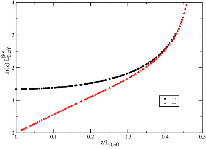
Figure 1: We plot $L_{0,eff}^{\beta/\nu}m(z)$ as a function of $z/L_{0,eff}$, where $z=x_{0}-(L_{0}+1)/2$ gives the distance from the middle of the film. The effective thickness of the film is $L_{0,eff}=L_{0}+L_{s}$ using $L_{s}=1.9$. For $++$ and $+-$ boundary conditions, data for films with $L_{0}\geq 16$ are used.

VI.3 Casimir force at the critical point

We have computed

$$\Delta f(L_{0},\beta_{c})=f(L_{0}+1/2,\beta_{c})-f(L_{0}-1/2,\beta_{c})$$ (46)

using the algorithm discussed in ref. yet . We have simulated $++$ and $+-$ boundary conditions on lattices of the thicknesses $L_{0}=6.5$, $7.5$, $8.5$, $9.5$, $10.5$, $11.5$, $12.5$, $13.5$, $15.5$, $19.5$, $23.5$, $27.5$, $31.5$ and $39.5$. For all these simulations, we have used $L\approx 8L_{0}$. We have checked that this is sufficient to avoid finite $L$ corrections. These simulations took in total about 10 month of CPU-time on one core of a Quad-Core AMD Opteron(tm) Processor 2378 running at 2.4 GHz. As update we have used the local heat bath algorithm. For lack of time and the still moderate amount of CPU time that was spent here, we made no effort to implement cluster updates or to implement the method using the multispin coding technique.

We have fitted our data with the ansätze

$$\Delta f(L_{0},\beta_{c})=f_{bulk}(\beta_{c})-\theta(0)\;(L_{0}+L_{s})^{-3}$$ (47)

and in order to check for the effect of subleading corrections to scaling

$$\Delta f(L_{0},\beta_{c})=f_{bulk}(\beta_{c})-\theta(0)\;(L_{0}+L_{s})^{-3}\times(1+c\;(L_{0}+L_{s})^{-2})\;\;.$$ (48)

Fitting with the ansatz (47) we get for the $++$ boundary conditions and $L_{0,min}=11.5$ the results $f_{bulk}(\beta_{c})=-0.0757368(3)$, $\theta(0)=-0.815(10)$, $L_{s}=1.86(5)$ and $\chi^{2}/$d.o.f.$=0.36$. Using the ansatz (48) and $L_{0,min}=6.5$ we get the results $f_{bulk}(\beta_{c})=-0.0757370(2)$, $\theta(0)=-0.824(5)$, $L_{s}=1.91(4)$ and $\chi^{2}/$d.o.f.$=0.51$.

Fitting with the ansatz (47) we get for the $+-$ boundary conditions and $L_{0,min}=11.5$ the results $f_{bulk}(\beta_{c})=-0.0757368(2)$, $\theta(0)=5.617(16)$, $L_{s}=1.930(13)$ and $\chi^{2}/$d.o.f.$=1.11$. Using the ansatz (48) and $L_{0,min}=6.5$ we get the results $f_{bulk}(\beta_{c})=-0.0757368(2)$, $\theta(0)=5.610(14)$, $L_{s}=1.912(17)$ and $\chi^{2}/$d.o.f.$=0.81$.

We notice that the results for $f_{bulk}(\beta_{c})$ obtained from the two different boundary conditions are consistent. We conclude

$$f_{bulk}(\beta_{c})=-0.0757368(4)\;\;.$$ (49)

Also the values for $L_{s}$ obtained here are fully consistent with the estimate $L_{s}=1.9(1)$ found above. As our result for the finite size scaling functions at the critical point of the bulk system we quote

$$\theta_{++}(0) = -0.820(15)$$ (50)

$$\theta_{+-}(0) = \phantom{+}5.613(20)\;\;.$$ (51)

Also here we have checked that the uncertainty of $\beta_{c}$ can be safely ignored. For a comparison of these results with previous ones given in the literature, see table 3 below.

VII Numerical results for the Casimir force in a large range of temperatures

Here we compute the Casimir force using the method discussed by Hucht Hucht . The details of the implementation are similar to myXY , where we have studied the thermodynamic Casimir force for films with free boundary conditions in the three dimensional XY universality class.

We have simulated the model for both types of boundary conditions and the thicknesses $L_{0}=8,9,16,17,32$ and $33$ for a large number of $\beta$-values in the neighborhood of the critical point. In tables 1 and 2 we give the $\beta$-values at which we have simulated and the statistics of our runs for the $+-$ and the $++$ boundary conditions, respectively. In the case of $+-$ boundary conditions we also give the lattice size $L$ that was used. Since for $+-$ boundary conditions the correlation length is increasing with increasing $\beta$ also $L$ has to increase with increasing $\beta$. In contrast, for $++$ boundary conditions, the correlation length stays rather small for all temperatures. It has a maximum quite close to the critical point. Therefore we have used $L=32$ for $L_{0}=8$, $9$, $L=64$ for $L_{0}=16$, $17$ and $L=128$ for $L_{0}=32$, $33$ at all values of $\beta$, where we have simulated at.

We have measured the energy per area. Using these data we have computed

$$\Delta E(L_{0},\beta)=E(L_{0}+1/2,\beta)-E(L_{0}-1/2,\beta)-E_{bulk}(\beta)\;\;.$$ (52)

The value for the energy density of the bulk system $E_{bulk}(\beta)$ is taken from simulations of $L^{3}$ or $2L\times L^{2}$ lattices with periodic boundary conditions in all three directions. The linear lattice size $L$ is taken sufficiently large to avoid significant finite size effects. For most values of $\beta$ simulated here we have also a direct measurement of $E_{bulk}(\beta)$. In a small neighborhood of $\beta_{c}$ we have used instead the result of a fit with the ansatz

$$E_{bulk}(\beta)=E_{ns}+C_{ns}(\beta-\beta_{c})+a_{\pm}|\beta-\beta_{c}|^{1-\alpha}+d_{ns}(\beta-\beta_{c})^{2}+b_{\pm}|\beta-\beta_{c}|^{2-\alpha}\;\;.$$ (53)

For a discussion see section IV A of myamplitude . Throughout the statistical error of $E_{bulk}(\beta)$ is clearly smaller than that of $E(L_{0}+1/2,\beta)-E(L_{0}-1/2,\beta)$. Also the systematical error caused by the interpolation with the ansatz  (53) can be safely ignored here.

In order to obtain $\Delta f_{ex}$ we have numerically integrated $\Delta E_{ex}$ using the trapezoidal rule:

$$-\Delta f_{ex}(\beta_{n})\approx\sum_{i=0}^{n-1}\frac{1}{2}(\beta_{i+1}-\beta_{i})\left(\Delta E_{ex}(\beta_{i+1})+\Delta E_{ex}(\beta_{i})\right)$$ (54)

where $\beta_{i}$ are the values of $\beta$ we have simulated at. They are ordered such that $\beta_{i+1}>\beta_{i}$ for all $i$. The starting point of the integration $\beta_{0}$ is chosen such that $\Delta E_{ex}(\beta_{0})=0$ within the statistical error.

The estimate obtained from the integration is affected by statistical and systematical errors. The statistical one can be easily computed, since the $\Delta E_{ex}$ are obtained from independent simulations:

$$\epsilon^{2}(-\Delta f_{ex}(\beta_{n})) = \frac{(\beta_{1}-\beta_{0})^{2}}{4}\epsilon^{2}[\Delta E_{ex}(\beta_{0})]+\frac{(\beta_{n}-\beta_{n-1})^{2}}{4}\epsilon^{2}[\Delta E_{ex}(\beta_{n})]$$ (55)

$$+ \sum_{i=1}^{n-1}\frac{(\beta_{i+1}-\beta_{i-1})^{2}}{4}\epsilon^{2}[\Delta E_{ex}(\beta_{i})]$$

where $\epsilon^{2}$ denotes the square of the statistical error.

In order to estimate the error due to the finite step size $\beta_{i+1}-\beta_{i}$ we have redone the integration, skipping every second value of $\beta$; i.e. doubling the step size. We find that the finite step size errors are at most of the size of the statistical ones.

Table 1: Statistics of our runs for the $+-$ boundary conditions. In the first column we give the thickness that is considered, where for example $L_{0}=8.5$ means that we have simulated films of the thicknesses $L_{0}=8$ and $9$. In the second column we give the linear extension $L$ of the lattice in 1 and 2 direction. We have simulated at $\beta_{i}=\beta_{min}+i\Delta\beta$ in the interval $[\beta_{min},\beta_{max}]$. In the last column we give the number of measurements for each of the simulations.

$L_{0}$	$L$	$\beta_{min}$	$\beta_{max}$	$\Delta\beta$	stat
8.5	32	0.25	0.325	0.005	200 000
8.5	32	0.33	0.348	0.002	200 000
8.5	32	0.35	0.38	0.001	200 000
8.5	32	0.381	0.385	0.001	300 000
8.5	64	0.385	0.43	0.001	150 000
8.5	96	0.43	0.46	0.002	100 000
8.5	128	0.46	0.5	0.002	100 000
8.5	256	0.505	0.56	0.005	100 000
16.5	64	0.34	0.348	0.002	200 000
16.5	64	0.35	0.384	0.001	200 000
16.5	64	0.385	0.395	0.0005	200 000
16.5	128	0.395	0.41	0.001	100 000
16.5	256	0.412	0.42	0.002	100 000
16.5	512	0.422	0.43	0.002	100 000
16.5	512	0.44	0.44	0.01	100 000
32.5	128	0.36	0.355	0.005	1 000 000
32.5	128	0.365	0.368	0.001	1 000 000
32.5	128	0.369	0.3875	0.0005	1 000 000
32.5	128	0.3875	0.39125	0.00025	1 000 000
32.5	256	0.3915	0.395	0.0005	250 000

Table 2: Statistics of our runs for the $++$ boundary conditions. The notation is the same as in the previous table for $+-$ boundary conditions. Here we have used $L=4(L_{0}-1/2)$ for all values of $\beta$.

$L_{0}$	$\beta_{min}$	$\beta_{max}$	$\Delta\beta$	stat
8.5	0.25	0.295	0.005	5 000 000
8.5	0.3	0.348	0.002	5 000 000
8.5	0.35	0.358	0.002	10 000 000
8.5	0.36	0.378	0.001	10 000 000
8.5	0.379	0.395	0.0005	10 000 000
8.5	0.396	0.409	0.001	10 000 000
8.5	0.41	0.43	0.002	10 000 000
16.5	0.31	0.33	0.01	10 000 000
16.5	0.34	0.352	0.002	10 000 000
16.5	0.354	0.379	0.001	10 000 000
16.5	0.38	0.382	0.0005	10 000 000
16.5	0.3825	0.39225	0.00025	10 000 000
16.5	0.393	0.399	0.001	10 000 000
16.5	0.4	0.406	0.002	10 000 000
32.5	0.37	0.375	0.001	10 000 000
32.5	0.376	0.3795	0.0005	10 000 000
32.5	0.38	0.3856	0.0002	10 000 000
32.5	0.3858	0.3889	0.0001	10 000 000
32.5	0.389	0.3918	0.0002	10 000 000
32.5	0.392	0.3945	0.0005	10 000 000
32.5	0.395	0.396	0.001	10 000 000

In figures 2 and 3 we have plotted our results for the finite size scaling functions $\theta_{+-}(x)$ and $\theta_{++}(x)$, respectively. The solid lines that are plotted linearly interpolate between the data points that we have computed. Note that the statistical error of $\Delta f_{ex}(L_{0})L_{0}^{3}$ is of similar size as the thickness of the line. In both cases, in the upper figure we do not take into account any correction to scaling. This means we plot $-\Delta f_{ex}(L_{0})L_{0}^{3}$ as a function of $t[L_{0}/\xi_{0}]^{1/\nu}$, using $\nu=0.63002$.

Not taking into account any correction, we see for both $++$ and $+-$ boundary conditions a clear discrepancy between the curves for $L_{0}=8.5$, $16.5$ and $32.5$.

Therefore in the lower part of the figures 2 and 3 we have replaced $L_{0}$ by $L_{0,eff}=L_{0}+L_{s}$, using the value $L_{s}=1.9$ obtained above from the finite size scaling study at the bulk critical point. This means that we have plotted $-\Delta f_{ex}(L_{0})(L_{0}+L_{s})^{3}$ as a function of $t[(L_{0}+L_{s})/\xi_{0}]^{1/\nu}$. Now the curves essentially fall on top of each other. Therefore we do not consider further corrections and take the curves obtained for $L_{0}=16.5$ and $32.5$ as our final result. The remaining small difference between $L_{0}=16.5$ and $32.5$ gives us some measure for the systematical error of our final result.

Now let us discuss the properties of $\theta_{++}(x)$ and $\theta_{+-}(x)$. We see that $\theta_{++}(x)$ is negative and $\theta_{+-}(x)$ is positive in the whole range of $x$. This means that in the case of $++$ boundary conditions the force is attractive, while for $+-$ boundary conditions it is repulsive. In both cases the function shows a single extremum. In the case of $++$ boundary conditions it is located in the high temperature phase, while for $+-$ it is in the low temperature phase. In order to accurately locate these extrema, we have computed the zeros of $\Delta E(L_{0},\beta)$. For $++$ boundary conditions we find $\beta_{min}=0.37407(3)$, $0.38219(2)$ and $0.38569(2)$ for $L_{0}=8.5$, $16.5$ and $32.5$, respectively. For these values of $\beta_{min}$ we have computed $x_{min}=t_{min}[(L_{0}+L_{s})/\xi_{0}]^{1/\nu}$ and correspondingly $\theta_{min}=-\Delta f_{ex}(\beta_{min})(L_{0}+L_{s})^{3}$. As our final result we take the value obtained for $L_{0}=32.5$ using $L_{s}=1.9$, $\nu=0.63002$ and $\xi_{0}=0.2282$. We arrive at

$$x_{++,min}=5.82(10)\;\;\;\;\;\theta_{++,min}=-1.76(3)\;\;,$$ (56)

where the quoted error takes into account the statistical error and the errors due to the uncertainties of $L_{s}$, $\xi_{0}$ and $\nu$.

For $+-$ boundary conditions we find $\beta_{max}=0.39961(2)$, $0.39256(2)$ and $0.389525(10)$ for $L_{0}=8.5$, $16.5$ and $32.5$, respectively. In the same way as above for $++$ boundary conditions we arrive at

$$x_{+-,max}=-5.17(7)\;\;\;\;\;\theta_{+-,max}=6.56(10)\;\;.$$ (57)

At the bulk critical point we get $\theta_{++}(0)=0.84(2)$ and $\theta_{+-}(0)=5.56(7)$. These results are less precise but fully consistent with those obtained in the previous section, eqs. (50,51).

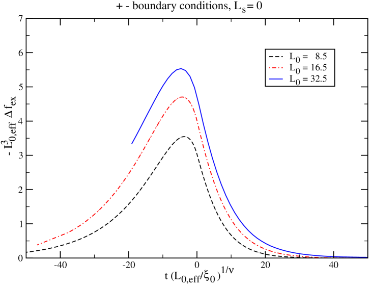
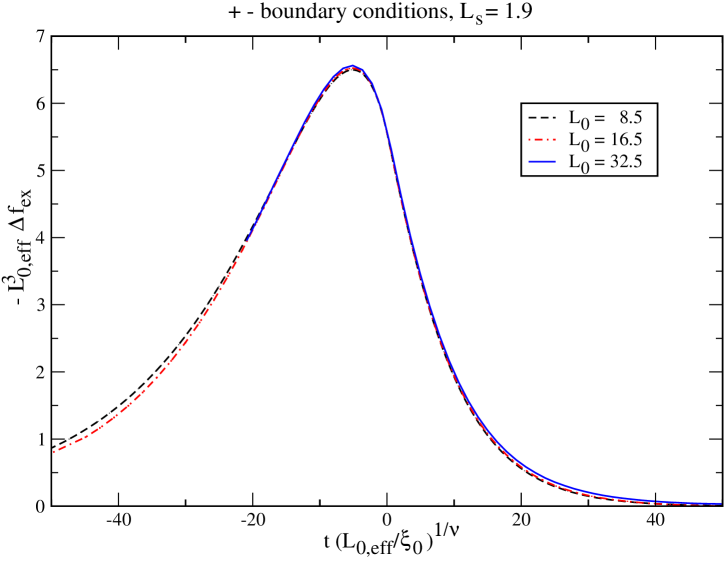
Figure 2: $+-$ boundary conditions. In the upper part of the figure we plot $-L_{0}^{3}\Delta f_{ex}$ as a function of $t(L_{0}/\xi_{0})^{1/\nu}$ for $L_{0}=8.5$, $16.5$ and $32.5$, where we use $\nu=0.63002$ and $\xi_{0}=0.2282$. In the lower part we have replaced $L_{0}$ by $L_{0,eff}=L_{0}+L_{s}$ with $L_{s}=1.9$. For a discussion see the text.

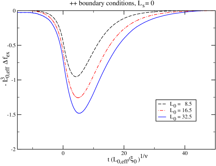
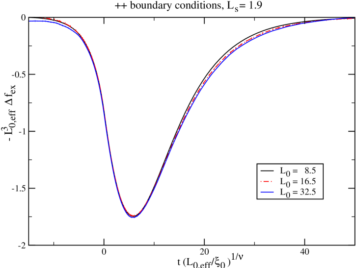
Figure 3: $++$ boundary conditions. In the upper part of the figure we plot $-L_{0}^{3}\Delta f_{ex}$ as a function of $t(L_{0}/\xi_{0})^{1/\nu}$ for $L_{0}=8.5$, $16.5$ and $32.5$, where we use $\nu=0.63002$ and $\xi_{0}=0.2282$. In the lower part we have replaced $L_{0}$ by $L_{0,eff}=L_{0}+L_{s}$ with $L_{s}=1.9$. For a discussion see the text.

In ref. myZZZZZ we have demonstrated at the example of films with periodic and free boundary conditions in the three dimensional XY universality class that the relation $\theta(x)=2h(x)-\frac{x}{\nu}h^{\prime}(x)$, eq. (19), can be employed to compute $\theta(x)$ from the excess energy per area of the film, without taking the derivative with respect to the thickness $L_{0}$ of the film.

The main practical problem of this approach is that for free boundary conditions as well as symmetry breaking boundary conditions that are studied here, the analytic part of the free energy per area and hence also of the energy per area suffers from a boundary correction that is not described by $L_{0,eff}=L_{0}+L_{s}$ of the singular part. In section VI.1 we have already determined the value of this correction at the bulk critical point. However it turns out that it is not sufficient here to approximate this correction by a constant. Even by adding a term linear in the reduced temperature $t$ to the analytic boundary correction, we could not reliably compute $\theta_{++}(x)$ and $\theta_{+-}(x)$. We made no attempt to improve this by adding higher order terms.

VII.1 Behavior at large $|x|$

In figure 4 we have plotted $\theta_{++}(x)$ and $-\theta_{+-}(x)$ in the high temperature phase. For comparison we have plotted $\theta_{++}(x)$ given by eq. (31). We have fixed the constant $C^{2}$ by matching the value at $x\approx 20$, where $\theta_{++}(x)$ and $-\theta_{+-}(x)$ still agree within the error bars. We find

$$C^{2}=1.5(1)\;\;.$$ (58)

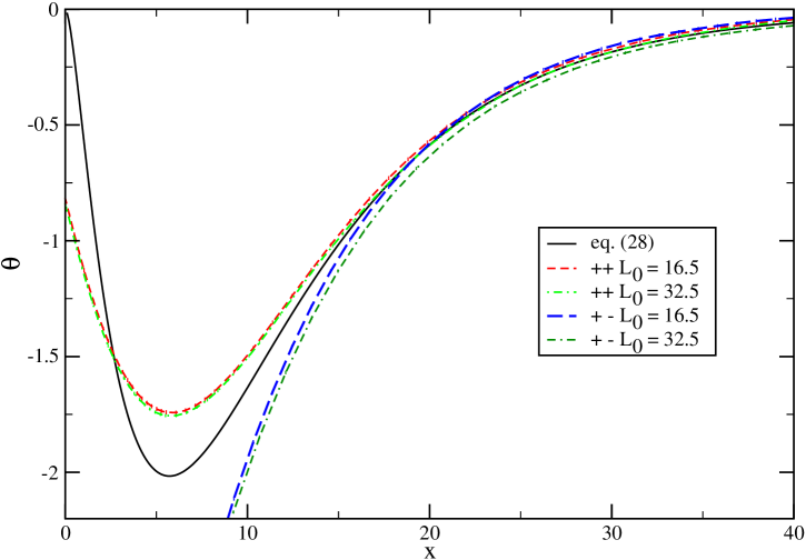
Figure 4: We plot our numerical results for $\theta_{++}(x)$ and $-\theta_{+-}(x)$ obtained with $L_{0}=16.5$ and $32.5$ using $L_{s}=1.9$ for $x>0$. For comparison we give the result of eq. (31), setting $C^{2}=1.5$. For a discussion see the text.

Indeed for $x\gtrapprox 20$ at the level of our accuracy $\theta_{++}(x)$ and $-\theta_{+-}(x)$ are equal. In the same range, the two curves are well approximated by eq. (31).

Next let us turn to the low temperature phase. We have matched eq. (33) with our numerical results obtained for $L_{0}=16.5$ and $32.5$ and $++$ boundary conditions at $x\approx-7$. We get

$$\bar{C}^{2}=0.20(5)\;\;.$$ (59)

As one can see from figure 5 there is reasonable match between our numerical results for $\theta_{++}(x)$ and eq. (33) for $x\lessapprox-5$. In figure 5 we have plotted the statistical error of our results. The fact that for small $x$, within less than two standard deviations, the estimate of $\theta_{++}(x)$ computed for $L_{0}=16.5$ and $L_{0}=32.5$ becomes equal to zero is a non-trivial validation of our numerical integration.

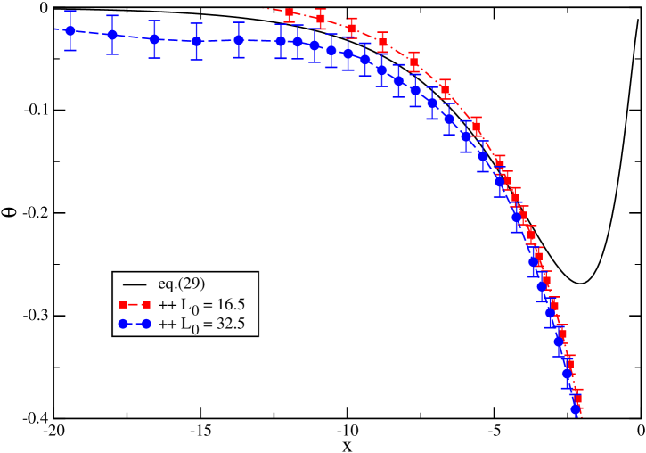
Figure 5: We plot our numerical results for $\theta_{++}(x)$ obtained with $L_{0}=16.5$ and $32.5$ using $L_{s}=1.9$ for $x<0$. For comparison we give the result of eq. (33), setting $\bar{C}^{2}=0.2$. For a discussion see the text.

VII.2 Correlation length of the films

For all simulations discussed above we have measured the second moment correlation length as defined in section III.3. The correlation length is interesting for practical purpose, since we have to choose the lattice size $L$ in 1 and 2 direction such that $L\gg\xi_{2nd}$ in order to avoid sizable effectively two dimensional finite size effects. Furthermore we shall discuss the finite size scaling behavior of the second moment correlation length of the film to further probe the theoretical expectations on corrections to scaling.

To this end, we have plotted in figure 6 for $++$ boundary conditions $\xi_{2nd}/L_{0,eff}$ of the film as a function of the scaling variable $x=t[L_{0,eff}/\xi_{0}]^{1/\nu}$ for the thicknesses $L_{0}=8$, $9$, $16$, $17$, $32$ and $33$. Using $L_{s}=1.9$ instead of $L_{s}=0$ clearly improves the collapse of the curves obtained from different thicknesses $L_{0}$. Using $L_{s}=1.9$, in the range $-20\gtrapprox x\gtrapprox 20$ the curves obtained for different thicknesses fall on top of each other within the error bars. For larger values of $x$ there is some discrepancy between the thicknesses $L_{0}=8$ and $9$ and $L_{0}=16$, $17$, $32$ and $33$ on the other hand. This can be attributed to analytic corrections to scaling. For all thicknesses $\xi_{2nd}/L_{0,eff}$ assumes a single maximum at $x\approx 7$.

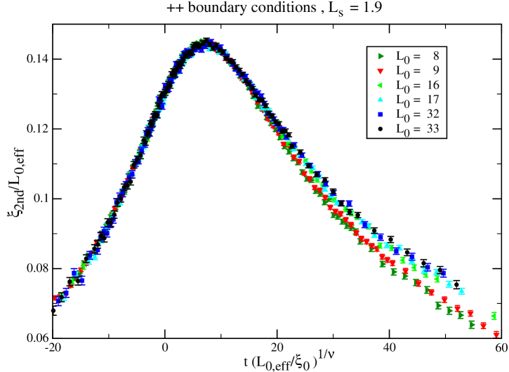
Figure 6: For $++$ boundary conditions, we plot $\xi_{2nd}/L_{0,eff}$ as a function of the scaling variable $x=t[L_{0,eff}/\xi_{0}]^{1/\nu}$ for $L_{0}=8$, $9$, $16$, $17$, $32$ and $33$ using $L_{s}=1.9$. Notice that $\xi_{2nd}$ is the second moment correlation length of the film, while $\xi_{0}$ appearing in the scaling variable $x$ is the amplitude of the correlation length of the bulk system in the high temperature phase.

Figure 7 is the analogue of figure 6 for $+-$ instead of $++$ boundary conditions. Also here we find, using $L_{s}=1.9$ a nice collapse of the curves obtained for the different thicknesses of the films. Now $\xi_{2nd}/L_{0,eff}$ is monotonically increasing with decreasing $x$. In figure 7 we have stopped, a bit arbitrary, at $x=-50$. For $x\approx-79.7$, the smallest value of $x$ that we have reached for $L_{0}=9$, we get $\xi_{2nd}/L_{0,eff}\approx 3.5$.

With an increasing correlation length the autocorrelation time of the Metropolis update increases. Therefore simulations become increasingly difficult as we go deeper into the low temperature phase, towards smaller values of $x$. As a consequence we had to stop at $x\approx-20.4$ and $-21.3$ for $L_{0}=32$ and $33$, respectively.

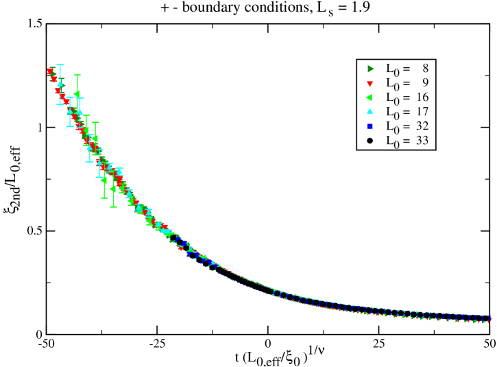
Figure 7: Same as figure 6 for $+-$ instead of $++$ boundary conditions.

VIII Comparison with other theoretical results and experiments

The scaling functions $\theta_{++}$ and $\theta_{+-}$ have been computed recently by using Monte Carlo simulations of the spin-1/2 Ising model on the simple cubic lattice VaGaMaDi07 ; VaGaMaDi08 . The results are presented in figures 3 and 4 of VaGaMaDi07 and 9 and 10 of VaGaMaDi08 for $++$ and $+-$ boundary conditions, respectively. For both types of boundary conditions, the final result depends strongly on the precise form of the ansatz, see eqs. (18,20,21,23) of VaGaMaDi08 , for corrections to scaling that is chosen. Qualitatively, the curves for both $++$ and $+-$ boundary conditions agree with ours. For the position of the extrema the authors of VaGaMaDi08 quote $x_{++,min}=5.90(8)$ and $x_{+-,max}=-5.4(1)$ in the caption of their figures 9 and 10, respectively. These are in quite good agreement with our results. In Nature ; GaMaHeNeHeBe09 , see the discussion below eq. (14) of GaMaHeNeHeBe09 , the authors extract the amplitude $C^{2}$ from the data of VaGaMaDi08 . Their result depends on the ansatz that is chosen for the corrections and also on the boundary conditions. Using the ansatz that is denoted by (i) in figures 9 and 10 of VaGaMaDi08 , they find $C^{2}=1.51(2)$ and $1.82(2)$ for $++$ and $+-$ boundary conditions, respectively. Instead, using the ansatz that is denoted by (ii) they arrive at $C^{2}=1.16(2)$ and $1.38(2)$, respectively. It is clear from these numbers that systematical errors due to corrections to scaling are much larger than statistical errors. Taking this into account, there is nice agreement with our estimate $C^{2}=1.5(1)$, eq. (58).

In figure 8 we compare our result for $\theta_{++}(x)$ with that obtained by using the de Gennes-Fisher local-functional method BoUp08 . As input the method uses universal amplitude ratios of the bulk system. Here we made no effort to redo the calculations of BoUp08 using our updated values for the universal amplitude ratios myamplitude and value for the exponent $\nu$ (Ref. mycritical ). Instead, we have copied the curve from figure 1 of BoUp08 . Overall we find a reasonable agreement with our result. We see a very small shift of the local-functional method curve towards larger values of $x$ compared with ours. Clearly, the value of the minimum of the curve obtained by the local-functional method is smaller than that of ours.

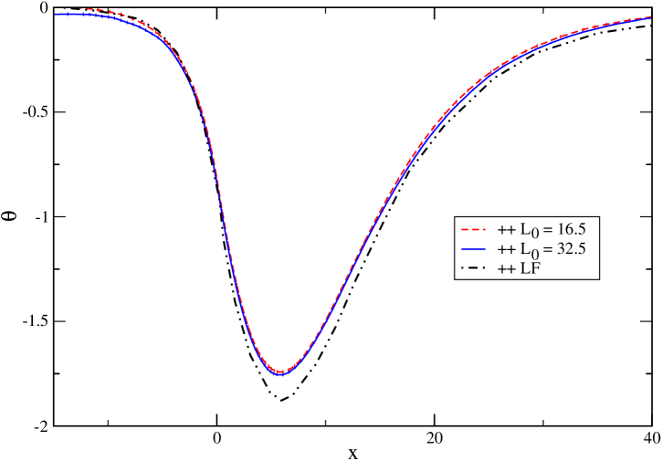
Figure 8: We plot the result of ref. BoUp08 for $\theta_{++}(x)$ obtained by using the de Gennes-Fisher local-functional (LF) method. We have copied the curve from fig. 1 of BoUp08 . For comparison we plot our numerical results for $\theta_{++}(x)$ obtained with $L_{0}=16.5$ and $32.5$ using $L_{s}=1.9$.

The authors of FuYaPe05 have studied wetting films of a binary mixture of methylcyclohexane and perfluoromethylcyclohexane. They have deduced the thermodynamic Casimir force from measurements of the thickness of the film. Their result for $\theta_{+-}(x)$ given in figure 3 of FuYaPe05 is more or less consistent with but much less precise than our result. The authors of Nature ; GaMaHeNeHeBe09 have studied the thermodynamic Casimir force between colloidal particles that are immersed into a mixture of water and lutidine and the surface of the cell. The surface of the particle was prepared such that it either preferentially absorbs water or lutidine. Hence both $++$ and $+-$ boundary conditions were accessible. A major problem in the interpretation of the experimental data is to disentangle the thermodynamic Casimir force from other forces. It turns out that only for relatively large $x$, reliable results could be obtained. Theoretically the colloidal particle and the surface of the cell are described by a sphere and a plane. In Nature ; GaMaHeNeHeBe09 the Derjaguin approximation had been used to obtain a prediction for this geometry starting from the theoretical results for the universal finite size scaling functions $\theta_{++}(x)$ and $\theta_{+-}(x)$ for the film geometry. The authors of Nature ; GaMaHeNeHeBe09 have fitted their data with the equivalent of ansatz (31), taking $\xi_{0}$ as free parameter. Their result for $\xi_{0}$ is consistent with that obtained from the analysis of bulk quantities. This check could be made more stringent by replacing the theoretical estimate of $C^{2}$ of Nature ; GaMaHeNeHeBe09 by ours eq. (58).

Finally in table 3 we have summarized results obtained for the scaling functions at the bulk critical point. In the literature, results obtained by field theoretic methods Krech97 , the de Gennes-Fisher local-functional method BoUp98 , Monte Carlo simulations Krech97 ; VaGaMaDi07 ; VaGaMaDi08 and experiment FuYaPe05 can be found. Mostly, in the original work, the so called Casimir amplitude $\Delta=\theta(0)/2$ is quoted. We see that field theoretic methods, in particular the $\epsilon$-expansion, are not able to provide quantitatively satisfying results. Those of the de Gennes-Fisher local-functional method BoUp98 are in much better agreement with ours. The results of previous Monte Carlo simulations differ by more than the quoted error bars from our results. Note that in ref. VaGaMaDi07 only the statistical error is quoted. The numbers quoted for VaGaMaDi08 are obtained by using an ansatz different from that of VaGaMaDi07 , which explains the difference between them. In figure 8 of VaGaMaDi08 the authors give in addition to the results obtained with their preferred ansatz those obtained by using two alternative ansätze. From this comparison one might conclude that the systematical error is larger than the statistical one that we quote in table 3.

As we have seen here, for the thicknesses that can be studied today, corrections to scaling, in particular those caused by the boundaries, are numerically important. In order to get an accurate result for the scaling limit, these corrections have to be properly taken into account. In the generic case, when corrections $\propto L_{0}^{-\omega}$, with $\omega=0.832(6)$, and $\propto L_{0}^{-1}$ are present this is a difficult task.

Table 3: Comparison of our results for $\theta_{++}(0)$ and $\theta_{+-}(0)$ with those given in the literature. For a discussion see the text.

Ref.	Method	$\theta_{++}(0)$	$\theta_{+-}(0)$
Krech97	$\epsilon$-expansion	-0.346	3.16
Krech97	$d=3$ expansion	-0.652	4.78
BoUp98	local-functional	-0.84(16)	6.2
FuYaPe05	experiment	–	6(2)
Krech97	Monte Carlo	-0.690(32)	4.900(64)
VaGaMaDi07	Monte Carlo	-0.884(16)	5.97(2)
VaGaMaDi08	Monte Carlo	-0.75(6)	5.42(4)
here	Monte Carlo	-0.820(15)	5.613(20)

IX Summary and Conclusions

We have studied the thermodynamic Casimir force for thin films in the three dimensional Ising universality class. In particular we have studied symmetry breaking boundary conditions. We consider the two cases $++$ and $+-$, where the fixed spins at the boundary are either all positive or are positive at one boundary and negative at the other. We have simulated the improved Blume-Capel model on the simple cubic lattice. The boundary conditions are expected to cause corrections that are to leading order $\propto L_{0}^{-1}$. In general it is hard to disentangle such corrections from leading corrections to finite size scaling which are $\propto L_{0}^{-\omega}$ where $\omega=0.832(6)$ (Ref. mycritical ). In the improved model, corrections to scaling $\propto L_{0}^{-\omega}$ are eliminated. This fact very much simplifies the analysis of the Monte Carlo data. In particular we could clearly demonstrate that the corrections caused by the boundaries can be expressed by an effective thickness $L_{0,eff}=L_{0}+L_{s}$. For our model we find, for both $++$ and $+-$ boundary conditions $L_{s}=1.9(1)$.

Having corrections to scaling well under control, we have obtained reliable results for the universal finite size scaling functions $\theta_{++}(x)$ and $\theta_{+-}(x)$, where $x=t[L_{0,eff}/\xi_{0}]^{1/\nu}$, of the thermodynamic Casimir force. For large values of $x$, we have compared our estimates for $\theta_{++}(x)$ and $\theta_{+-}(x)$ with the prediction (31) derived by using the transfer matrix formalism. We find good agreement. For large values of $-x$ we have compared $\theta_{++}(x)$ with eq. (33) also derived by using the transfer matrix formalism. Also here we find agreement.

Finally we have compared our estimates for $\theta_{++}(x)$ and $\theta_{+-}(x)$ with field theoretic calculations, the de Gennes-Fisher local-field method, previous Monte Carlo simulations and experiments. While field theory does not provide quantitatively satisfying results, those of the local-field method are in quite reasonable agreement with ours. Also the results of previous Monte Carlo simulations are essentially in agreement with ours.

X Acknowledgements

This work was supported by the DFG under the grant No HA 3150/2-1.

References

- (1) K. G. Wilson and J. Kogut, Phys. Rep. C 12, 75 (1974).
- (2) M. E. Fisher, Rev. Mod. Phys. 46, 597 (1974).
- (3) M. E. Fisher, Rev. Mod. Phys. 70, 653 (1998).
- (4) A. Pelissetto and E. Vicari, Phys. Rept. 368, 549 (2002) [arXiv:cond-mat/0012164].
- (5) M. E. Fisher and P.-G. de Gennes, CR Seances Acad. Sci. Ser. B 287, 207 (1978).
- (6) A. Gambassi, J. Phys. Conf. Ser. 161, 012037 (2009) [arXiv:0812.0935].
- (7) Krech M, The Casimir Effect in Critical Systems (World Scientific, Singapore, 1994)
- (8) K. Binder, “Critical Behaviour at Surfaces” in Phase Transitions and Critical Phenomena, Vol. 8, eds. C. Domb and J. L. Lebowitz, (Academic Press, 1983)
- (9) H. W. Diehl, Field-theoretical Approach to Critical Behaviour at Surfaces in Phase Transitions and Critical Phenomena, edited by C. Domb and J.L. Lebowitz, Vol. 10 (Academic, London 1986) p. 76.
- (10) H. W. Diehl, Int. J. Mod. Phys. B 11, 3503 (1997) [arXiv:cond-mat/9610143].
- (11) M. N. Barber, “Finite-size Scaling” in Phase Transitions and Critical Phenomena, Vol. 8, eds. C. Domb and J. L. Lebowitz, (Academic Press, 1983)
- (12) M. Hasenbusch, A Finite Size Scaling Study of Lattice Models in the 3D Ising Universality Class, [arXiv:1004.4486].
- (13) T. W. Burkhardt and H. W. Diehl, Phys. Rev. B 50, 3894 (1994).
- (14) U. Nellen, L. Helden, and C. Bechinger Europhys. Lett. 88, 26001 (2009) [arXiv:0910.2373].
- (15) T. F. Mohry, A. Maciołek, and S. Dietrich, Phys. Rev. E 81, 061117 (2010) [arXiv:1004.0112].
- (16) O. Vasilyev, A. Gambassi, A. Maciołek, and S. Dietrich, Europhys. Lett. 80, 60009 (2007) [arXiv:0708.2902].
- (17) O. Vasilyev, A. Gambassi, A. Maciołek, and S. Dietrich, Phys. Rev. E 79, 041142 (2009) [arXiv:0812.0750].
- (18) Z. Borjan and P. J. Upton, Phys. Rev. Lett. 81, 4911 (1998) .
- (19) Z. Borjan and P. J. Upton, Phys. Rev. Lett. 101, 125702 (2008) [arXiv:0804.2340].
- (20) Y. Deng and H. W. J. Blöte, Phys. Rev. E 70, 046111 (2004).
- (21) M. Hasenbusch, Universal amplitude ratios in the 3D Ising Ising Universality Class, [arXiv:1004.4983].
- (22) M. Campostrini, A. Pelissetto, P. Rossi and E. Vicari, Phys. Rev. E 65, 066127 (2002) [cond-mat/0201180].
- (23) K. E. Newman and E. K. Riedel, Phys. Rev. B 30, 6615 (1984).
- (24) M. Campostrini, A. Pelissetto, P. Rossi and E. Vicari, Phys. Rev. E 57, 184 (1998) [arXiv:cond-mat/9705086].
- (25) T. W. Capehart and M. E. Fisher, Phys. Rev. B 13, 5021 (1976).
- (26) H. W. Diehl, S. Dietrich, and E. Eisenriegler, Phys. Rev. B 27, 2937 (1983).
- (27) M. Kikuchi and Y. Okabe, Prog. Theor. Phys. 73, 32 (1985).
- (28) M. Krech, Phys. Rev. B 62, 6360 (2000) [arXiv:cond-mat/0006448] and references therein; H. W. Diehl, M. Krech, and H. Karl, Phys. Rev. B 66, 6360 (2002) [arXiv:cond-mat/0203368].
- (29) V. Agostini, G. Carlino, M. Caselle, and M. Hasenbusch, Nucl. Phys. B 484, 331 (1997) [arXiv:hep-lat/9607029].
- (30) S. Klessinger and G. Münster, Nucl. Phys. B 386, 701 (1992) [arXiv:hep-lat/9205028].
- (31) R. Evans and J. Stecki, Phys. Rev. B 49, 8842 (1994).
- (32) M. Krech, Phys. Rev. E 56, 1642 (1997) [arXiv:cond-mat/9703093].
- (33) R. C. Brower and P. Tamayo, Phys. Rev. Lett. 62, 1087 (1989).
- (34) R. H. Swendsen and J.-S. Wang, Phys. Rev. Lett. 58, 86 (1987).
- (35) U. Wolff, Phys. Rev. Lett. 62, 361 (1989).
- (36) See, e.g., S. Wansleben, J. B. Zabolitzky, and C. Kalle, J. Stat. Phys. 37, 271 (1984); G. Bhanot, D. Duke, and R. Salvador, Phys. Rev. B 33, 7841 (1986).
- (37) M. Hasenbusch and S. Meyer, Phys. Rev. Lett. 66, 530 (1991).
- (38) M. Saito and M. Matsumoto, “SIMD-oriented Fast Mersenne Twister: a 128-bit Pseudorandom Number Generator”, in Monte Carlo and Quasi-Monte Carlo Methods 2006, edited by A. Keller, S. Heinrich, H. Niederreiter, (Springer, 2008); M. Saito, Masters thesis, Math. Dept., Graduate School of schience, Hiroshima University, 2007. The source code of the program is provided at “http://www.math.sci.hiroshima-u.ac.jp/m-mat/MT/SFMT/index.html”
- (39) M. Hasenbusch, Phys. Rev. E 80, 061120 (2009) [arXiv:0908.3582].
- (40) A. Hucht, Phys. Rev. Lett. 99, 185301 (2007) [arXiv:0706.3458].
- (41) M. Hasenbusch, J. Stat. Mech.: Theory Exp. 2009, P07031 [arXiv:0905.2096].
- (42) M. Hasenbusch, Phys. Rev. B 81, 165412 (2010) [arXiv:0907.2847].
- (43) M. Fukuto, Y. F. Yano and P. S. Pershan, Phys. Rev. Lett. 94, 135702 (2005).
- (44) C. Hertlein, L. Helden, A. Gambassi, S. Dietrich, and C. Bechinger, Nature (London) 451, 172 (2008).
- (45) A. Gambassi, A. Maciołek, C. Hertlein, U. Nellen, L. Helden, C. Bechinger, and S. Dietrich, Phys. Rev. E 80, 061143 (2009) [arXiv:0908.1795].