The finite-width Laplace sum rules for $0^{++}$ scalar glueball in instanton liquid model

Abstract

In the framework of a semi-classical expansion for quantum chromodynamics in the instanton liquid background, the correlation function of the $0^{++}$ scalar glueball current is given. Besides the pure classical and quantum contributions, the contributions arising from the interactions between the classical instanton fields and quantum gluons are taken into account as well. Instead of the usual zero-width approximation for the resonance, the Brite-Wigner form for the spectral function of the finite-width resonance is adopted. The family of the Laplace sum rules for the scalar glueball in quantum chromodynamics with and without light quarks are studed. A consistency between the subtracted and unsubtracted sum rules are very well justified, and the values of the mass, decay width, and the coupling to the corresponding current for the $0^{++}$ resonance in which the glueball fraction is dominant, are obtained.

1 Introduction

Understanding the nature of the lightest state of glueballs, the $0^{++}$ scalar glueball, is a long-standing puzzle in QCD[1, 2]. The mass scale of this glueball is predicted to be within the region of 1.30 -1.75GeV by quenched Lattice QCD[3, 4, 5, 6, 7], and by un- quenched lattice QCD[8, 9, 10]. Up to now, there has not been clear evidence for the observation of a scalar glueball, while the closest scalar candidates are $f_{0}(1370)$, $f_{0}(1500)$ and $f_{0}(1700)$[1, 11]. More nonperturbative physics is needed in the theoretical and phenomenological investigation on such area.

Laplace sum rule[12] calculations of glueball properties can be based on correlation functions involving interpolating field, which is not as much successful in the prediction of scalar glueball mass as in the ones of other hadron properties in the early days with the inconsistency between the subtracted[13, 14, 15, 16, 17] and unsubtracted[18, 19] sum rules(SSR and USSRs). Instanton vacuum should be included in the scalar tunnel[20, 21, 22] to offer the main non-perturbative effects.

Instantons are the localized solutions of the classical Euclidean field equations with finite minimized action [23]. They can be solved by constructing the self-dual or self-antidual field configurations classified by different topological charges. The perturbative theory should be carried out around these classical solutions with the average zero-topological charge instead of the trivial one, which is the kernel of the semiclassical expansion method.

Not all the hadrons alike[20]. Instanton contributions should not be neglected at least in the scalar and pseudoscalar channels. Direct instanton contributions are already included in sum rule approaches[24, 25, 26, 27, 28, 29] based on the instanton liquid model of the QCD vacuum[31, 30]. The compatibility between the resultant USSRs and SSR for the scarlar glueball is greatly improved, but still not be very satisfying. It should be noticed that, in the so-called direct instanton approximation, the interactions between instantons and the pure quantum gluon fields are not considered, and the procedure is criticized by involving with the problem of double counting[25], because in the correlator are included both contributions coming from condensates and instantons, but the latter could lead to the formation of the former.

The interactions between the classical and quantum gluon field configurations are always ignored[24, 25, 26, 27, 28, 29] because the interactive effects were expected to be small[26]. However, there is no reasonable argument before an actual calculation. We have found that these interactive effects are, in fact, compatible with or even important more than that of the condensate and the perturbative effects at least in the $0^{++}$ channel. Moreover, including the classical, quantum and interactive effects in the framework of the semiclassical expansion of the instanton background, the stability and the consistency for the SSR and USSRs for $0^{++}$ scalar glueball could be arrived [32].

Motivated by the above considerations, our main purpose in this paper is to investigate the $0^{++}$ glueball in the frame work of Laplace sum rules. To avoid the problem of double counting, instead of using the scheme of the mixture of the traditional condensates and the so-called direct instanton contribution, we are working in the framework of the semiclassical expansion of QCD in the instanton liquid vacuum, which is a well-defined self-consistent procedure for the quantum theory justified by the path-integral quantization formalism. For the correlation function, we include the contributions from the interactions between the quantum gluons and the classical instanton background besides the ones coming from only instantons and from only quantum gluons. For the spectral function, beyond the usual zero-width approximation, we adopt the Breit-Wigner form for the considered resonance with correct threshold behavior, in order to get the information of not only the mass scale but also the full decay width.

2 Correlation function

The correlation function for the scalar glueball in Euclidean space-time with the virtuality $q^{2}$ is defined by

$$\Pi(q^{2})=\int\textrm{d}^{4}x\textrm{e}^{iq\cdot x}\langle\Omega|TO_{s}(x)O_{s}(0)|\Omega\rangle,$$ (1)

where $|\Omega\rangle$ is the physical vacuum, and the scalar glueball current $O_{s}$ of the quantum numbers $J^{PC}=0^{++}$ is given by

$$O_{s}=\alpha_{s}G^{a}_{\mu\nu}(B)G^{a,\mu\nu}(B),$$ (2)

with $\alpha_{s}$ being the strong coupling constant, it is gauge-invariant, and renormalization invariant at one-loop-level. On spirit of the semiclassical expansion, and in order to maintain the $O(4)$-covariance, the gluon field strength tensor $G^{a}_{\mu\nu}(B)$ is considered as a functional of the full gluon potential $B_{\mu a}=A_{\mu a}+a_{\mu a}$ with $A_{\mu a}$ and $a_{\mu a}$ being the instanton fields and the corresponding quantum fluctuations.

The theoretical expression, $\Pi^{\textrm{QCD}}$, for the correlation function $\Pi$ may be divided into the following three parts

$$\Pi^{\textrm{QCD}}(Q^{2})=\Pi^{\textrm{inst}}(Q^{2})+\Pi^{\textrm{int}}(Q^{2})+\Pi^{\textrm{pert}}(Q^{2}),$$ (3)

where $Q^{2}=q^{2}$, and $\Pi^{\textrm{inst}}(Q^{2})$, $\Pi^{\textrm{pert}}(Q^{2})$, and $\Pi^{\textrm{int}}(Q^{2})$ are the contributions from the pure instatons, the pure perturbation QCD, and the interactions between the instantons and the quantum gluon fields, respectively. We note that we have not included here the contributions from the so-called condensates because at first in a systematic semiclassical expansion of QCD, the non-perturbative effects are parameterized by the classical instanton and anti-instanton solutions of the equation of motion of QCD, and at second we want to avoid the double counting problem due to the fact that some condensates can be reproduced from the instanton contributions, and thirdly, we have checked that the condensates contributions are negligible in comparison with the contributions considered here.

The perturbative contribution $\Pi^{\textrm{pert}}(Q^{2})$ up to three-loop level in the chiral limit of QCD is already known to be

$$\Pi^{\textrm{pert}}(Q^{2})=Q^{4}\ln\left(\frac{Q^{2}}{\mu^{2}}\right)\left[a_{0}+a_{1}\ln\left(\frac{Q^{2}}{\mu^{2}}\right)+a_{2}\ln^{2}\left(\frac{Q^{2}}{\mu^{2}}\right)\right],$$ (4)

where $\mu^{2}$ is the renormalization scale in the $\overline{\mbox{MS}}$ dimensional regularization scheme, and the coefficients with the inclusion of the threshold effects are

$$a_{0} = -2\left(\frac{\alpha_{s}}{\pi}\right)^{2}\left[1+\frac{659}{36}\left(\frac{\alpha_{s}}{\pi}\right)+247.48\left(\frac{\alpha_{s}}{\pi}\right)^{2}\right],$$

$$a_{1} = 2\left(\frac{\alpha_{s}}{\pi}\right)^{3}\left[\frac{9}{4}+65.781\left(\frac{\alpha_{s}}{\pi}\right)\right],\quad a_{2}=-10.1252\left(\frac{\alpha_{s}}{\pi}\right)^{4}$$ (5)

for QCD with three quark flavors up to three-loop level in the chiral limit [28, 29, 33], and

$$a_{0}=-2\left(\frac{\alpha_{s}}{\pi}\right)^{2}\left[1+\frac{51}{4}\left(\frac{\alpha_{s}}{\pi}\right)\right],\quad a_{1}=\frac{11}{2}\left(\frac{\alpha_{s}}{\pi}\right)^{3},\quad a_{2}=0$$ (6)

for quarkless QCD up to two-loop level [34]. Both expressions for $\Pi^{\textrm{pert}}(Q^{2})$ with and without quark loop corrections are used in our calculation for comparison. With the assumption that the dominant contribution to $\Pi^{\textrm{inst}}(Q^{2})$ comes from BPST single instanton and anti-instanton solutions [23, 35, 36] and the multi-instanton effects are negligible [26], and in view of the gauge-invariance of the correlation function, one may choose to work in the regular gauge of the classical single instanton potential

$$A^{a}_{\mu}=\frac{2}{g_{s}}\eta^{a}_{\mu\nu}\frac{(x-x_{0})_{\nu}}{(x-x_{0})^{2}+\rho^{2}},$$ (7)

where $\eta^{a}_{\mu\nu}$ is the ’t Hooft symbol, and $x_{0}$ and $\rho$ denote the position and size of the instanton, respectively. The pure instaton contribution is obtained to be [13, 24, 25, 37, 38, 39, 40]

$$\Pi^{\textrm{inst}}(Q^{2})=2^{5}\pi^{2}\bar{n}\bar{\rho}^{4}Q^{4}K^{2}_{2}(\sqrt{Q^{2}}\bar{\rho}),$$ (8)

where $K_{2}(x)$ is the McDonald function, $\bar{n}=\int_{0}^{\infty}d\rho n(\rho)$ and $\bar{\rho}$ are the overall instanton density and the average instanton size in the random instanton background, respectively.

It is noticed that the contribution to $\Pi$ from the interactions between instantons and the quantum gluon fields is of the order of the product of $\alpha_{s}$ and the overall instanton density $\bar{n}$. There is no reason to get rid off this contribution in comparison with the perturbative contributions of the higher order $\alpha_{s}^{4}$ considered in $\Pi^{\textrm{pert}}$. To calculate such contribution, our key observation is that the instanton potential $A^{a}_{\mu}$ obeys also the fixed-point gauge condition

$$(x-x_{0})_{\mu}A^{a}_{\mu}(x-x_{0})=0,$$ (9)

due to the anti-symmetricity of the ’t Hooft symbols. As a consequence, the instanton potential can be expressed in terms of the corresponding field strength tensor as follows

$$A^{a}_{\mu}(x-x_{0})=\int_{0}^{1}duuF^{a}_{\mu\nu}[u(x-x_{0})](x-x_{0})_{\nu},$$ (10)

and the gauge-link with respect to the instanton fields is just the unit operator, and thus the trace of any product of the gauge-covariant instanton field strengths at different points is gauge-invariant. This allows us to conclude that the remainder quantum corrections to the gauge-invariant correlation function, arising from the interactions between the instantons and the quantum gluons, is gauge-invariant as well. Therefore, one may choose any specific gauge in evaluating the quantum correction to $\Pi^{\textrm{int}}$. Working in Feynman gauge, our results for $\Pi^{\textrm{int}}$ is

$$\Pi^{\textrm{int}}(Q^{2})=C_{0}\alpha_{s}\bar{n}\pi+\alpha_{s}^{2}\bar{n}\left\{C_{1}+[C_{2}(Q\bar{\rho})^{2}+C_{3}]\ln(Q\bar{\rho})^{2}+\frac{C_{4}}{(Q\bar{\rho})^{2}}\right\},$$ (11)

where the coefficients are:

$$C_{0}=62.62,\,\,C_{1}=1533.15,\,\,C_{2}=825.81,$$

$$C_{3}=-496.33,\,\,C_{4}=-348.89.$$ (12)

It is remarkable to note that the fixed point $x_{0}$, which characterizes the gauge condition (10), disappears in the expression of $\Pi^{\textrm{int}}$, as expected from the gauge-invariance of our procedure.

3 Spectral function

Turn to construct the spectral function for the correlation function of the scalar glueball current. The usual lowest one resonance plus a continuum model is used to saturate the phenomenological spectral function,

$$\textrm{Im}\Pi^{\textrm{PHE}}(s)=\rho^{\textrm{had}}(s)+\theta(s-s_{0})\textrm{Im}\Pi^{\textrm{QCD}}(s),$$ (13)

where $s_{0}$ is the QCD-hadron duality threshold, $\rho^{\textrm{had}}(s)$ the spectral function for the lowest scalar glueball state, and the imaginary part of the correlation function Eq. (3), $\textrm{Im}\Pi^{\textrm{QCD}}(s)$, is

$$\textrm{Im}\Pi^{\textrm{QCD}}(s) = -\pi s^{2}\left[a_{0}+2a_{1}\ln\frac{s}{\mu^{2}}+\left(3\ln^{2}\frac{s}{\mu^{2}}-\pi^{2}\right)a_{2}\right]$$ (14)

$$-16\pi^{4}s^{2}\bar{n}\bar{\rho}^{4}J_{2}(\bar{\rho}\sqrt{s})Y_{2}(\bar{\rho}\sqrt{s})+\alpha_{s}^{2}\bar{n}\pi(C_{2}\bar{\rho}^{2}s-C_{3}).$$

Instead of using the zero-width approximation as usual, the Brite-Wigner form for $n$ resonances is adopted for $\rho^{\textrm{had}}(s)$

$$\rho^{\textrm{had}}(s)=\sum_{i=1}^{n}\frac{f_{i}^{6}m_{i}\Gamma_{i}}{(s-m^{2}_{i}+\Gamma^{2}_{i}/4)^{2}+m_{i}^{2}\Gamma_{i}^{2}},$$ (15)

where $f^{3}_{i}=\langle\Omega|O_{s}|0^{++}_{i}\rangle$ is the coupling of the $i$’s resonance to the glueball current (2). Recall the threshold behavior for $\rho^{\textrm{had}}(s)$

$$f^{3}_{i}\rightarrow\lambda_{0}s\hskip 20.0pt\mbox{for }s\rightarrow 0,$$ (16)

with the value of $\lambda_{0}$ being fixed by the low-energy theorem of QCD[13, 18, 20, 41], and thus independent of what an individual resonance considered. The early QCD sum rule approach had often used $f^{3}_{i}\rightarrow\lambda_{0}s$ (with $n=1$) in the whole lowest resonance region, however the obtained mass scale is too low to be expected from lattice QCD simulations. In fact, the threshold behavior (16) is valid in the chiral limit, it may not be extrapolated far away. Therefore, instead of considering the couplings $f_{i}$ as constants [26], we choose the model for $f$ as

$$f^{3}_{i}=\left\{\begin{array}[]{ll}\lambda_{0}s&\mbox{for }s<m^{2}_{\pi},\\ \lambda_{0}m^{2}_{\pi}+\lambda^{3}_{i}&\mbox{for }s\geq m^{2}_{\pi},\end{array}\right.$$ (17)

with $\lambda_{i}$ being some constants, so that the spectral function $\rho^{\textrm{had}}(s)$ has the almost complete Breit-Wigner form with correct threshold behavior which is important to maintain the convergence of the integral for the spectral function of the $k=-1$ sum rule.

4 Finite-width Laplace sum rules

A family of Laplace sum rules with different $k$-moments can be constructed from the Borel transformation, $\hat{\mathcal{B}}$, to the correlation function (3)[12]

$$\mathcal{L}^{\textrm{had}}_{k}(s_{0},t)=\mathcal{L}^{\textrm{QCD}}_{k}(s_{0},t)+\Pi(0)\delta_{k,-1},$$ (18)

where $s_{0}$ is the threshold for setting on the continuum, $\Pi(0)$ is come from the subtraction to the corresponding dispersion relation due to the degree of divergence of the correlation function of the scalar glueball, and

$$\mathcal{L}^{\textrm{QCD}}_{k}(s_{0},t) = t\hat{\mathcal{B}}\left[(-Q^{2})^{k}\Pi^{\textrm{QCD}}(Q^{2})\right]-\int^{\infty}_{s_{0}}\textrm{d}ss^{k}e^{-s/t}\frac{1}{\pi}\Pi^{\textrm{QCD}}(s),$$ (19)

$$\mathcal{L}^{\textrm{had}}_{k}(s_{0},t) = \int^{s_{0}}_{0}\textrm{d}ss^{k}e^{-s/t}\frac{1}{\pi}\rho^{\textrm{had}}(s).$$ (20)

The Laplace sum rule emphasizes the contribution from the lowest hadron state considered, and suppresses the higher resonance contributions and the continuum exponentially.

For $k=-1,0$ and $1$, a straightforward manipulation leads to

$$\mathcal{L}^{\textrm{QCD}}_{-1}(t) = \left[-a_{0}+(2\gamma-2)a_{1}-0.5(6\gamma^{2}-12\gamma-\pi^{2})a_{2}\right]t^{2}+2^{7}\pi^{2}\bar{n}$$ (21)

$$-2^{6}\pi^{2}\bar{n}x^{2}\textrm{e}^{-x}\left[(1+x)K_{0}(x)+\left(2+x+\frac{2}{x}\right)K_{1}(x)\right]$$

$$-C_{0}\bar{n}\pi\alpha_{s}+\bar{n}\alpha_{s}^{2}[-C_{1}+C_{2}\bar{\rho}^{2}t+C_{3}(\gamma-\ln(\bar{\rho}^{2}t))-\frac{C_{4}}{\bar{\rho}^{2}t}],$$

$$\mathcal{L}^{\textrm{QCD}}_{0}(t) = \left[-2a_{0}+(4\gamma-6)a_{1}-(6\gamma^{2}-18\gamma-\pi^{2}+6)a_{2}\right]t^{3}$$ (22)

$$+2^{7}\pi^{2}\bar{n}\frac{x^{5}}{\bar{\rho}^{2}}\textrm{e}^{-x}\left[2K_{0}(x)+\left(2+\frac{1}{x}\right)K_{1}(x)\right]$$

$$+\bar{n}\alpha_{s}^{2}[C_{2}\bar{\rho}^{2}t^{2}-C_{3}t+C_{4}/(\bar{\rho}^{2})],$$

$$\mathcal{L}^{\textrm{QCD}}_{1}(t) = \left[-6a_{0}+(12\gamma-22)a_{1}-(18\gamma^{2}-66\gamma-3\pi^{2}+36)a_{2}\right]t^{4}$$ (23)

$$+2^{8}\pi^{2}\bar{n}\frac{x^{6}}{\bar{\rho}^{4}}\textrm{e}^{-x}\left[(9-4x)K_{0}(x)+\left(7-4x+\frac{3}{x}\right)K_{1}(x)\right]$$

$$+\bar{n}\alpha_{s}^{2}[2C_{2}\bar{\rho}^{2}t^{3}-C_{3}t^{2}],$$

where $x=\bar{\rho}^{2}t/2$.

5 Numerical calculation

Now, we specify the input parameters in numerical calculation. We take the color and flavor numbers to be $N_{c}=3$ and $N_{f}=3$, respectively. The expressions for two-loops quarkless ($N_{f}=0$) running coupling constant $\alpha_{s}(Q^{2})$ at renormalization scale $\mu$ [42, 43] and for the three-loop running coupling constant with three flavors ($N_{f}=3$) are used, where the central value of the $\overline{\textrm{MS}}$ QCD scale $\Lambda$ is taken to be $120$ MeV. We recall here that a research on the renormalization group improvement for Laplace sum rules amount to choose the renormalization scale to be $\mu^{2}=t$ [44]. The subtraction constant $\Pi(0)$ is determined by low-energy theorem [13]

$$\Pi(0)=\frac{32\pi}{9}\langle\alpha_{s}G^{2}\rangle\simeq 0.6\,\textrm{GeV}^{4},$$ (24)

which leads to $\lambda_{0}=5.0$GeV. The values of the average instanton size and the overall instanton density are adopted from the instanton liquid model

$$\bar{n}=1\,\textrm{fm}^{-4}=0.0016\,\textrm{GeV}^{4},\,\,\,\bar{\rho}=\frac{1}{3}\,\textrm{fm}=1.689\,\textrm{GeV}^{-1}.$$ (25)

Finally, the mass of the neutral pion is taking from the experimental data, i.e. $m_{\pi}=135$ MeV.

To determining the values of the resonance parameters appearing in Eq.(15), we match both sides of sum rules (18) optimally in the fiducial domain. The conditions for determining the value of $s_{0}$ are: first, it should be grater than $m^{2}$; second, it should guarantee that there exists a sum rule window for our Laplace sum rules. We note that the upper limit $t_{\textrm{max}}$ of the sum rule window is determined by requiring that the contribution from the continuum should be less than that of the resonance

$$\mathcal{L}^{\textrm{cont}}_{k}(s_{0},t_{\textrm{max}})\leq\mathcal{L}^{\textrm{QCD}}_{k}(s_{0},t_{\textrm{max}}),$$ (26)

while the lower limit $t_{\textrm{min}}$ of the sum rule window is obtained by requiring the contribution of pure instantons to be greater than 50% of $\mathcal{L}^{\textrm{QCD}}_{k}(s_{0},t)$, because such classical contributions should be dominant in the low-energy region. Moreover, to require that the multi-instanton corrections remain negligible, we simply adopt a rough estimate

$$t_{\textrm{min}}^{-1}\leq(2\bar{\rho})^{2}\sim({2}/{0.6\textrm{GeV}})^{2}.$$ (27)

In order to measure the compatibility between both sides of the sum rules (18) realized in our numerical simulation, we introduce a variation, $\delta$, defined by

$$\delta=\frac{1}{N}\sum_{1}^{N}\frac{[L(t_{i})-R(t_{i})]^{2}}{|L(t_{i})R(t_{i})|},$$ (28)

where the interval $[t_{\textrm{min}},t_{\textrm{max}}]$ is divided into $100$ equal small intervals, $N=101$, and $L(t_{i})$ and $R(t_{i})$ are l.h.s and r.h.s of Eq.(18) evaluated at $t_{i}$.

In the world of quarkless QCD there is only one well defined scalar bound state of gluons below 1GeV suggested by lattice QCD, and thus we choose $n=1$ in Eq.(15). Including quarks enhances the difficulty of the task since many states possessing the same quantum numbers may present in the correlator. The assumption of a single well-isolated lowest resonance is questioned from the admixture with quarkonium states, and from the experimental data that three $0^{++}$ scalar states around the mass scale of $1500$MeV, namely $f_{0}(1370)$, $f_{0}(1500)$ and $f_{0}(1710)$. Therefore, we choose $n=3$ for $\rho^{\textrm{had}}(s)$. With the requirements mentioned above, the optimal parameters governing the sum rules are listed in Tab.LABEL:tab:3BWR.

Table 1: The fitting values of the mass $m$(GeV) and width $\Gamma$(GeV) of the possible $0^{++}$ resonances, and of the parameters $\lambda$(GeV), $f$(GeV) and $s_{0}$(GeV²) characterizing the couplings to the corresponding resonances and the continuum threshold, as well as of the sum rule window of $t$(GeV²) and the compatibility measure $\delta$ for finite-width Laplace sum rules (18) in the quarkless QCD (shown in the first three lines), as well as in QCD with three massless quarks (shown in the remainder lines, where the first three lines for $n=1$, and the others for $n=3$).

• $k$	$m$	$\Gamma$	$\lambda$	$f$	$s_{0}$	$[t_{\textrm{min}},t_{\textrm{max}}]$	$\delta$ ($10^{-5}$)
  $-1$	1.47	0.16	1.525	1.538	4.1	$[1.3,3.0]$	$4.39$
  0	1.49	0.13	1.519	1.532	4.5	$[1.6,6.0]$	$2.32$
  1	1.53	0.09	1.529	1.540	4.1	$[1.0,2.2]$	$2.23$
  $-1$	1.47	0.16	1.586	1.598	4.4	$[1.0,4.0]$	$1.25$
  0	1.48	0.13	1.612	1.624	4.3	$[1.5,4.6]$	$1.63$
  1	1.52	0.09	1.620	1.632	4.9	$[1.0,2.5]$	$5.12$
  	1.34	0.25	0.100	0.452
  $-1$	1.47	0.16	1.585	1.597	4.5	$[1.0,4.0]$	$1.67$
  	1.65	0.14	0.150	0.455
  	1.35	0.23	0.110	0.451
  0	1.47	0.12	1.607	1.619	4.2	$[1.5,4.5]$	$0.59$
  	1.70	0.13	0.200	0.463
  	1.38	0.25	0.150	0.456
  1	1.54	0.09	1.629	1.640	4.3	$[1.0,2.8]$	$4.69$
  	1.71	0.14	0.230	0.469

The corresponding curves for the l.h.s. and r.h.s. of (18) of $k=-1$, $0$ and $+1$ in quarkless QCD for $n=1$, and in QCD with three massless quarks for $n=3$ are displayed in Figs.1 and 2, respectively. These figurations show the consistent match between the both sides of Eq. (18) for $k=-1,0$ and $1$ respectively, with the corresponding fitting parameters. The solid lines are the r.h.s.(QCD) of Eq. (18), and the dashed lines are the l.h.s.(HAD) of Eq. (18), while the dotted line for the r.h.s. (QCD) excluding the contribution of interactions between the instantons and the quantum gluons. The matching between both sides of the sum rules are very well over the whole fiducial region with a very little departure. In the case of QCD with three massless quarks, the curves for $n=1$ are similar to those for $n=3$ with little worse compatibility, and not displayed here.

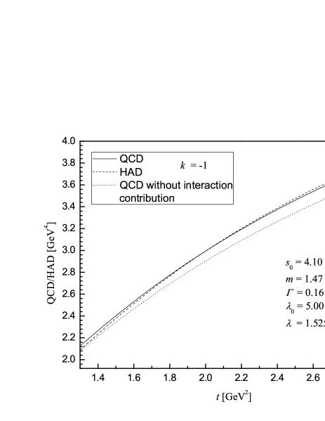
Figure 1: The curves for the l.h.s. and r.h.s. of the Eq. (18) for $k=-1$, $0$ and $+1$ cases of quarkless QCD with only the lowest resonance considered. The solid line denotes the r.h.s. (QCD), dashed line for l.h.s. (HAD), and dotted line for the r.h.s. (QCD) the without interaction contribution.

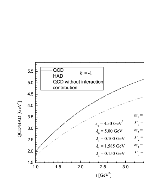
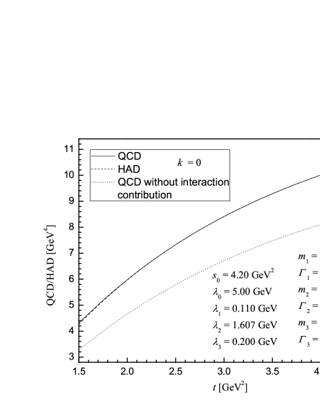
Figure 2: The curves for the l.h.s. and r.h.s. of the Eq. (18) for $k=-1$, $0$ and $+1$ cases of QCD with three massless quarks and the lowest three resonances considered. The solid line denotes the r.h.s. (QCD), dashed line for l.h.s. (HAD), and dotted line for the r.h.s. (QCD) the without interaction contribution.

6 Conclusion and discussion

The properties of $0^{++}$ glueball are examined in a family of the finite-width Laplace sum rules. The correlation function is calculated in a semiclassical expansion, a well-defined process justified in the path-integral quantization formalism, of QCD in the instanton background, namely the instanton liquid model of the QCD vacuum. Besides the contributions from pure gluons and instantons separately, the one arising from the interactions between the classical instanton fields and the quantum gluon ones are taken into account as well. Instead of using the usual zero-width approximation for the spectral function of the considered resonances, the Breit-Wigner form for the resonances with a correct threshold behavior is adopted. With the QCD standard input parameters, three Laplace sum rules with $k=-1,0,1$ are carefully studied.

By taking the average for the values, listed in tab. 1, of the corresponding $k=-1$, $0$ and $1$ sum rules, for the case of $n=1$, the values of the mass and width, and the other optical fit parameters are

$$m=1.51\pm 0.15\textrm{GeV},\,\Gamma=0.12\pm 0.04\textrm{GeV},$$

$$f=1.52\pm 0.12\,\textrm{GeV},\,s_{0}=4.5\pm 0.5\,\textrm{GeV}^{2}$$

in quarkless QCD, and

$$m=1.50\pm 0.15\textrm{GeV},\,\Gamma=0.12\pm 0.04\textrm{GeV},$$

$$f=1.61\pm 0.11\,\textrm{GeV},\,s_{0}=4.5\pm 0.5\,\textrm{GeV}^{2}$$

for QCD with three massless flavors, where the errors are estimated from the uncertainties of the spread between the individual sum rules, and by varying the phenomenological parameters, $\Lambda$ and $\langle\alpha_{s}G^{2}\rangle$, appropriately away from their central values $\Lambda=120-200\,\textrm{MeV}$ and $\langle\alpha_{s}G^{2}\rangle=0.6-0.8\textrm{GeV}^{4}$. It is remarkable to notice that these two results are close in value, and it indicates that the considered quark effects may be not so large at the energy scale of the resonance mass above 1GeV.

The above conclusion is further justified in the investigation of the case of $n=3$. We can see that the current is coupled mainly to the resonance state near $f_{0}(1500)$ predicted in a single resonance approach. To be quantitative, let us consider the case with the most excellent compatibility, namely the $k=0$ results shown in Tab.LABEL:tab:3BWR and Fig.2. The corresponding couplings $f^{6}$ to the three resonances $R_{1}$, $R_{2}$ and $R_{3}$ with masses $1.35$GeV, $1.47$GeV and $1.70$GeV are

$$0.092\textrm{GeV}^{3},\,\,\,4.073\textrm{GeV}^{3},\,\,\,0.094\textrm{GeV}^{3}$$ (29)

respectively, Note that

$$\left(\begin{array}[]{l}\langle 0|O_{s}|R_{1}\rangle\\ \langle 0|O_{s}|R_{2}\rangle\\ \langle 0|O_{s}|R_{3}\rangle\end{array}\right)=M\left(\begin{array}[]{l}\langle 0|O_{s}|1\rangle\\ \langle 0|O_{s}|8\rangle\\ \langle 0|O_{s}|G\rangle\end{array}\right)$$ (30)

where $M$ stands for the mixing matrix (s. the second one of Eqs.(45) in Ref.[11]). The values of the couplings of $O_{s}$ to the $\bar{q}q$ states $|1\rangle$, $|8\rangle$ and the pure glueball state $|G\rangle$ are

$$\langle 0|O_{s}|1\rangle=-0.48\,\textrm{GeV}^{3},$$

$$\langle 0|O_{s}|8\rangle=0.19\,\textrm{GeV}^{3},$$ (31)

$$\langle 0|O_{s}|G\rangle=0.86\,\textrm{GeV}^{3}$$

after normalization, respectively. Although the estimation is relatively rough, it is still remarkable to notice that, first, the coupling to $|G\rangle$ is dominant; and second, the signs of the couplings to $|1\rangle$ and $|8\rangle$ is consistent with the scalar glueball-meson coupling theorems[13, 20, 51].

As summary, we may conclude that the values of the mass and decay width of the $0^{++}$ resonance, in which the fraction of the scalar glueball state is dominant, are $m=1.5\pm 0.15$ GeV and $\Gamma=0.12\pm 0.03$ GeV, respectively, and the value of its coupling to the corresponding current is $\lambda_{s\geq m^{2}_{\pi}}=1.5\pm 0.12\ \,\textrm{GeV}$. They are not only compatible with lattice QCD simulation [3, 4, 5, 6, 7] and other estimation[24, 25, 26, 46, 47], but also in good accordance with the experimental data of $f_{0}(1500)$ [48, 49, 50].

It is also remarkable that the three Laplace sum rules lead to almost the same results, a consistency between the subtracted and unsubtracted sum rules are very well justified. We note that we have not working within the mixed scheme, namely with including condensates, and in the same time, adopting the so-called direct instanton approximation, but simply with a self-consistent framework, a quantum theory in a classical background, without the problem of double counting. In this aspect, our results further justified the instanton liquid model for QCD among other many justifications.

In our semiclassical expansion, the leading contribution to the sum rules comes from instantons themselves, especially in the region below the threshold $s_{0}$. It is the amount of this contribution determining the low-bound of the sum rule window. This means that the non-linear configurations of gluons have a dominant role with respect to the quantum fluctuations in the low-energy region.

The contribution of the interactions between the classical instanton fields and quantum gluon ones, considered in this letter but neglected in earlier sum rule calculations [24, 25, 28, 29, 46], is in fact not negligible. To the contrast, its amount is approximately double or even triple of that from the pure quantum fluctuations in the whole fiducial domain, expected from a view point of the semiclassical expansion. Moreover, it is obviously seen from Figs. 1-2 that, without taking the contribution from the interactions between instantons and quantum gluons into account, the departures between $\mathcal{L}^{\textrm{had}}_{k}(s_{0},t)$ and $\mathcal{L}^{\textrm{QCD without interaction}}_{k}(s_{0},t)$ become large, and all the three Laplace sum rules become less stable, and thus less reliable.

Finally, it should be noticed that the imaginary part of instanton contribution is an oscillating, amplificatory and nonpositive defined function, and so is the imaginary part of the correlation function. This property which is a fatal problem for the QCD sum rule calculation with the instanton background, may make the contribution of continuum too large to be under control. Hilmar Forkel introduced a Gaussian distribution for instanton to get rid off this trouble, and obtained a smaller $0^{++}$ mass scale: $1.25\pm 0.2$ GeV [24] compared to the earlier result $1.53\pm 0.2$ GeV [25]. We didn’t use this Gaussian distribution, but simply choose a smaller fitting parameter to avoid this problem.

References

References

- [1] Klempt E and Zaitsev A 2007 Phys. Rep. 454 1
- [2] Mathieu V, Kochelev N and Vento V 2009 Int. J. Mod. Phys. E 18 1
- [3] Morningstar C J and Peardon M 1999 Phys. Rev. D 60 034509
- [4] Xiang-Fei Meng and Gang Li et al. 2009 Phys. Rev. D 80 114502
- [5] Chen Y et al. 2006 Phys. Rev. D 73 014516
- [6] Vaccarino A and Weingarten D 1999 Phys. Rev. D 60 114501
- [7] Sexton J, Vaccarino A and Weingarten D 1995 Phys. Rev. Lett. 75 4563
- [8] [SESAM and TXL] Bali G S et al. 2000 Phys. Rev. D 62 054503(arXiv:hep-lat/0003012)
- [9] [UKQCD] MCNeile C and Michael C 2001 Phys. Rev. D 63 114503 (arXiv:hep-lat/0010019)
- [10] [UKQCD] Hart A and Teper M 2002 Phys. Rev. D 65 034502 (arXiv:hep-lat/0108022)
- [11] Crede V and Meyer C A 2009 Prog. Part. Nucl. Phys. 63 74
- [12] Shifman M A, Vainshtein A I and Zakharov V I 1979 Nucl. Phys. B 147 385, 448
- [13] Novikov V A, Shifman M A, Vainshtein A I and Zakharov V I 1980 Nucl. Phys. B 165 67
- [14] Liu Jueping and Liu Dunhuan 1993 J. Phys. G: Nucl. Part. Phys. 19 373
- [15] Liu Jueping and Liu Dunhuan 1991 Chin. Phys. Lett. 8 551
- [16] Bades J, Giminez V and Penarrocha J A 1989 Phys. Lett. B 223 251
- [17] Dominguez C A and Paver N 1986 Z. Phys. C 31 591
- [18] Shifman M A 1981 Z. Phys. C 9 347
- [19] Pascual P and Tarrach R 1982 Phys. Lett. B 113 495
- [20] Novikov V A, Shifman M A, Vainsthein A I and Zakharov V I 1981 Nucl. Phys. B 191 301
- [21] Geshkenbein B V and Ioffe B L 1980 Nucl. Phys. B 166 340
- [22] Shuryak E V 1983 Nucl. Phys. B 214 237
- [23] Belavin A, Polyakov A, Schwartz A and Tyupkin Y 1975 Phys. Lett. B 59 85
- [24] Forkel H 2005 Phys. Rev. D 71 054008
- [25] Forkel H 2001 Phys. Rev. D 64 034015
- [26] Schefer T and Shuryak E V 1995 Phys. Rev. Lett. 75 1707
- [27] Kisslinger L S and Johnson M B 2001 Phys. Lett. B 523 127
- [28] Harnett D, Steele T G and Elias V 2001 Nucl. Phys. A 686 393
- [29] Harnett D and Steele T G 2001 Nuc. Phys. A 695 205
- [30] Schefer T and Shuryak E V 1998 Rev. Mod. Phys. 70 323
- [31] Diakonov D I 2003 Prog. Part. Nucl. Phys. 51 173
- [32] Zhang Zhen-Yu and Liu Jue-Ping 2006 Chin. Phys. Lett. 23 2920
- [33] Chetyrkin K G, Kneihl B A and Steinhauser M 1997 Phys. Rev. Lett. 79 353
- [34] Bagan E and Steele T G 1990 Phys. Lett. B 234 135; Phys. Lett. B 243 413
- [35] ‘t Hooft G 1976 Phys. Rev. D 14 3432
- [36] Callan C G, Dashen R and Gross D 1978 Phys. Rev. D 17 2717
- [37] Harnett D, Steele T G and Elias V, Nucl. Phys. A 686 393
- [38] Shuryak E V 1982 Nucl. Phys. B 203 116
- [39] Geshkenbein B V and Ioffe B L 1980 Nucl. Phys. B 166 340
- [40] Ioffe B L and Samsonov A V 2000 Phys. At. Nucl. 63 1527
- [41] Novikov V A and Shifman M A 1981 Z. Phys. C 8 43
- [42] Groom D E et al. 2000 Eur. Phys. J. C 15 1
- [43] Prosperi G M, Raciti M and Simolo C 2007 Prog. Part. Nucl. Phys. 58 387 (arXiv:hep-ph/0607209)
- [44] Narison S and de Rafael E 1981 Phys. Lett. B 103 57
- [45] Giacosa F et al. 2005 Phys. Rev. D 72 094006 (arXiv:hep-ph/0509247)
- [46] Narison S 1998 Nucl. Phys. B 509 312
- [47] Liang Y and Liu K F et al. 1993 Phys. Lett. B 307 375
- [48] Amsler C et al. 2008 Phys. Lett. B 667 1
- [49] Amsler C and Close F E 1995 Phys. Lett. B 353 385
- [50] Amsler C et al. 1995 Phys. Lett. B 355 425
- [51] Kisslinger L S, Parno D and Riordan S 2008 Advances in High Energy Physics Vol 2008 (Artical ID 982341, Hindawi Publishing Corporation)