Anderson localization of a Tonks-Girardeau gas in potentials with controlled disorder

Abstract

We theoretically demonstrate features of Anderson localization in the Tonks-Girardeau gas confined in one-dimensional (1D) potentials with controlled disorder. That is, we investigate the evolution of the single particle density and correlations of a Tonks-Girardeau wave packet in such disordered potentials. The wave packet is initially trapped, the trap is suddenly turned off, and after some time the system evolves into a localized steady state due to Anderson localization. The density tails of the steady state decay exponentially, while the coherence in these tails increases. The latter phenomenon corresponds to the same effect found in incoherent optical solitons.

I Introduction

The phenomenon of Anderson localization Anderson1958 , which was originally theoretically predicted in the context of condensed matter physics, has been experimentally demonstrated in other wave systems including optical waves Wiersma1997 ; Chabanov2000 ; Storzer2006 ; Schwartz2007 ; Lahini2008 and ultracold atomic gases (matter waves) Billy2008 ; Roati2008 . In the context of Bose-Einstein condensates (BECs), Anderson localization was obtained by placing ultracold atomic BECs in elongated, essentially one-dimensional disordered Billy2008 and quasiperiodic incommensurate potentials Roati2008 , which were created optically (see Ref. Sanchez-Palencia2010 for a recent review of the topic). The matter waves utilized in those experiments were condensates, i.e., they were spatially coherent in the sense that their one-body density matrix factorizes $\rho(x_{1},x_{2})\approx\Phi^{*}(x_{1})\Phi(x_{2})$, where $\Phi(x)$ is the condensate wave function. However, in reality interactions and/or the presence of the thermal cloud affects the spatial coherence in the system. Naturally, the spatial coherence in the system is expected to have important implications on localization phenomena, since the phenomenon of Anderson localization is deeply connected to interference of multiple reflected waves. This motivates us to study Anderson localization in a Tonks-Girardeau gas, which is a relatively simple example of partially-spatially-coherent Bose gas (i.e., it is not condensed).

The Tonks-Girardeau model describes a system of strongly repulsive (”impenetrable”) bosons, confined in one-dimensional (1D) geometry Girardeau1960 . Exact solutions of the model are found by employing the Fermi-Bose mapping Girardeau1960 ; Girardeau2000 , wherein the Tonks-Girardeau wave function (for both the stationary and the time-dependent problems) is constructed from a wave function describing noninteracting spinless fermions. In Ref. Olshanii98 it was suggested that the Tonks-Girardeau model can be experimentally realized with ultracold atoms in effectively 1D atomic waveguides. This regime is reached at low temperatures, for sufficiently tight transverse confinement, and with strong effective interactions Olshanii98 ; Petrov2000 ; Dunjko2001 . Indeed, in 2004 two groups have experimentally realized the Tonks-Girardeau gas Kinoshita2004 ; Paredes2004 . Furthermore, nonequilibrium dynamics of a 1D Bose gas (including the Tonks-Girardeau regime) has been experimentally addressed in the context of relaxation to equilibrium Kinoshita2006 . It is known that ground states of the Tonks-Girardeau gas on the ring Lenard1964 , or in a harmonic potential Forrester2003 are not condensates, because the population of the leading natural orbital scales as $\sqrt{N}$, where $N$ is the number of particles. Thus, the Tonks-Girardeau gas is only partially spatially coherent. The free expansion of the Tonks-Girardeau gas from some initial state has been of great interest over the past few years Rigol2005exp ; Minguzzi2005 ; DelCampo2006 ; Gangardt2007 ; this type of scenario, i.e., expansion from an initial state which is localized (say by a trapping potential) can be used to address Anderson localization Billy2008 .

The experimental demonstrations of Anderson localization in ultracold atomic gases were preceded by theoretical investigations of this topic (e.g., see Refs. Damski2003 ; Roth2003 ; Sanchez-Palencia2007 , see also Ref. Sanchez-Palencia2010 and references therein). The interplay of disorder (or quasiperiodicity) and interactions in a Bose gas (from weakly up to strongly correlated regimes), has been often studied in the context of the Bose-Hubbard model Damski2003 ; Roth2003 ; Giamarchi1988 ; Fisher1989 ; Gimperlein2005 ; deMartino2005 ; Scarola2006 ; Rey2006 ; Horstmann2007 ; Roux2008 ; Deng2008 ; Roscilde2008 ; Orso2009 . Within the model, a transition from a superfluid to a Bose glass phase has been predicted to occur Giamarchi1988 ; Fisher1989 . The aforementioned interplay has been studied by using versatile methods including calculating the energy absorption rate Orso2009 , momentum distribution and correlations deMartino2005 ; Deng2008 , and expansion dynamics Horstmann2007 ; Roux2008 . In the limit of strong repulsion, the system can be described by using hard-core bosons on the lattice deMartino2005 ; Horstmann2007 ; Orso2009 . For these systems, by employing the Jordan-Wigner transformation the bosonic system is mapped to that of noninteracting spinless fermions, and all one-body observables can be furnished from the one body density matrix both in the stationary (e.g., see Rigol2005 ) and out-of-equilibrium systems Rigol2005exp . The ground state properties of the hard-core Bose gas in a random lattice have been studied in deMartino2005 , whereas expansion dynamics was considered in Horstmann2007 ; both approaches predict the loss of quasi long-range order.

Here we study Anderson localization within the framework of the Tonks-Girardeau model Girardeau1960 in one-dimensional disordered potentials. We study the expansion of a Tonks-Girardeau wave packet in a potential with controlled disorder. The potential is characterized by its correlation distance parameter $\sigma$. At $t=0$, the initial wave packet is in the ground state of a harmonic trap with frequency $\omega$ (with small disorder superimposed upon it), and then the trap is suddenly turned off. After some time, we find that the system reaches a steady state characterized by exponentially decaying tails of the density. We show that the exponents decrease with the increase of $\omega$ and the decrease of $\sigma$ in the investigated parameter span ($\sigma=0.13-0.40$ $\mu$m and $\omega=5-10$ Hz). The one-body density matrix $\rho_{B}(x,y,t)$ of the steady state, that is its amplitude $|\rho_{B}(0,x,t)|$, decays exponentially on the tails of the localized wave packet. However, in the region of these tails the degree of first order coherence $|\mu_{B}(0,x,t)|=|\rho_{B}(0,x,t)|/\sqrt{\rho_{B}(0,0,t)\rho_{B}(x,x,t)}$ reaches a plateau. These plateaus are connected to the behavior of the single-particle states used to construct the Tonks-Girardeau wave function, from which we find that the spatial coherence increases in the tails. This increase of coherence in the tails has its counterpart in incoherent optical solitons IncOpt , a phenomenon well understood in terms of the modal theory for incoherent light IncOpt .

The paper is organized as follows: In Section II we describe the Tonks-Girardeau model. In Section III we present our numerical results on Anderson localization in this system. Finally, in Section IV we outline our conclusions.

II Tonks-Girardeau model

In this section we present the Tonks-Girardeau model which describes ”impenetrable-core” 1D Bose gas Girardeau1960 ; Girardeau2000 . We study a system of $N$ identical Bose particles in 1D geometry, which experience an external potential $V(x)$. The bosons interact with impenetrable pointlike interactions Girardeau1960 , which means that the wave function describing the bosons vanishes whenever two particles are in contact, that is, $\psi_{B}(x_{1},x_{2},\ldots,x_{N},t)=0$ if $x_{i}=x_{j}$ for any $i\neq j$. The wave function $\psi_{B}$ must also obey the Schrödinger equation

$$i\frac{\partial\psi_{B}}{\partial t}=\sum_{j=1}^{N}\left[-\frac{\partial^{2}}{\partial x_{j}^{2}}+V(x_{j})\right]\psi_{B};$$ (1)

here we use dimensionless units as in Ref. Buljan2006 , i.e., $x=X/X_{0}$, $t=T/T_{0}$, and $V(x)=U(X)/E_{0}$, where $X$ and $T$ are space and time variables in physical units, and $U(X)$ is the potential in physical units. Given the particle mass $m$, the time scale $T_{0}=2mX_{0}^{2}/\hbar$ and energy-scale $E_{0}=\hbar^{2}/(2mX_{0}^{2})$ are set by choosing an arbitrary spatial length-scale $X_{0}$. For example, in our calculations below $X_{0}=1\ \mu$m, while the mass corresponds to ⁸⁷Rb, which yields the temporal scale $T_{0}=2.76\times 10^{-3}\ s$, and the energy scale $E_{0}=3.82\times 10^{-32}\ J$. The wave functions are normalized as $\int dx_{1}\ldots dx_{N}|\psi_{B}(x_{1},x_{2},\ldots,x_{N},t)|^{2}=1$.

The solution of this system may be written in compact form via the famous Fermi-Bose mapping, which relates the Tonks-Girardeau bosonic wave function $\psi_{B}$ to an antisymmetric many-body wave function $\psi_{F}$ describing a system of noninteracting spinless fermions in 1D Girardeau1960 :

$$\psi_{B}=\Pi_{1\leq i<j\leq N}\mbox{sgn}(x_{i}-x_{j})\psi_{F}(x_{1},x_{2},\ldots,x_{N},t).$$ (2)

In many physically relevant situations, the fermionic wave function $\psi_{F}$ can be written in a form of the Slater determinant,

$$\psi_{F}(x_{1},\ldots,x_{N},t)=\frac{1}{\sqrt{N!}}\det_{m,j=1}^{N}[\psi_{m}(x_{j},t)],$$ (3)

where $\psi_{m}(x,t)$ denote $N$ orthonormal single-particle wave functions obeying a set of uncoupled single-particle Schrödinger equations

$$i\frac{\partial\psi_{m}}{\partial t}=\left[-\frac{\partial^{2}}{\partial x^{2}}+V(x)\right]\psi_{m}(x,t),\ m=1,\ldots,N.$$ (4)

In Eqs. (2)-(4) we have outlined the construction of the many-body wave function describing the Tonks-Girardeau gas in an external potential $V(x)$, both in the static Girardeau1960 and time-dependent case Girardeau2000 .

Given the wave function $\psi_{B}$, we can straightforwardly calculate all one-body observables furnished by the reduced single-particle density matrix (RSPDM),

$$\rho_{B}(x,y,t) = N\int\!\!dx_{2}\ldots dx_{N}\,\psi_{B}(x,x_{2},\ldots,x_{N},t)^{*}$$ (5)

$$\times\psi_{B}(y,x_{2},\ldots,x_{N},t);$$

by employing the formalism presented in Ref. Pezer2007 . If the RSPDM is expressed in terms of the single-particle wave functions $\psi_{m}$ as

$$\rho_{B}(x,y,t)=\sum_{i,j=1}^{N}\psi^{*}_{i}(x,t)A_{ij}(x,y,t)\psi_{j}(y,t),$$ (6)

it can be shown that the $N\times N$ matrix ${\mathbf{A}}(x,y,t)=\{A_{ij}(x,y,t)\}$ has the form

$${\mathbf{A}}(x,y,t)=({\mathbf{P}}^{-1})^{T}\det{\mathbf{P}},$$ (7)

where the entries of the matrix ${\mathbf{P}}$ are $P_{ij}(x,y,t)=\delta_{ij}-2\int_{x}^{y}dx^{\prime}\psi_{i}^{*}(x^{\prime},t)\psi_{j}(x^{\prime},t)$ ($x<y$ without loss of generality) Pezer2007 .

III Numerical results on Anderson localization in a Tonks-Girardeau gas

In order to investigate Anderson localization of the Tonks-Girardeau gas, we perform numerical simulations designed in the fashion of optical Schwartz2007 and matter wave Billy2008 experiments which were conducted recently to demonstrate Anderson localization. We investigate dynamics of a Tonks-Girardeau wave packet in a disordered potential $V_{D}$(x), where the initial wave packet (at $t=0$) is localized in space by some trapping potential. After long time of propagation the wave packet reaches some steady state. Anderson localization is indicated by the exponential decay of the density of the wave packet in this steady state.

More specifically, we assume that initially, at $t=0$, the gas is in the ground state of the harmonic oscillator potential, with the small controlled disordered potential superimposed upon it, that is,

$$V(x)=V_{D}(x)+\nu^{2}x^{2}\mbox{ for $t<0$.}$$ (8)

At $t=0$ the trapping potential is suddenly turned off, i.e.,

$$V(x)=V_{D}(x)\mbox{ for $t>0$,}$$ (9)

after which the density and correlations of the gas begin to evolve. This means that at $t=0$ the wave function $\psi_{B}$ is given by Eqs. (2) and (3) where $\psi_{m}(x,t=0)$ is the $m$th single-particle eigenstate of the potential $V_{D}(x)+\nu^{2}x^{2}$. The subsequent evolution of $\psi_{m}$ is given by Eq. (4) where the potential is given solely by the disordered term $V(x)=V_{D}(x)$.

The construction of the disordered potential $V_{D}(x)$ used in our numerical simulations is described in the Appendix. The disordered potential can be characterized in terms of its correlation functions; the autocorrelation function is defined by

$$A_{C}(x)=\langle\overline{V}_{D}(x^{\prime}-x)\overline{V}_{D}(x^{\prime})\rangle_{x^{\prime}},$$ (10)

where $\overline{V}_{D}(x)=V_{D}(x)-\langle V_{D}(x^{\prime})\rangle_{x^{\prime}}$, and $\langle\cdots\rangle_{x^{\prime}}$ denotes a spatial average over $x^{\prime}$. For the disordered potentials in our simulations we have approximately

$$A_{C}(x)=V_{0}^{2}\frac{\sin^{2}(x/\sigma)}{(x/\sigma)^{2}},$$ (11)

where $\sigma$ denotes the spatial correlation length of the disordered potential, whereas $V_{0}^{2}=\langle\overline{V}^{2}_{D}(x)\rangle_{x}$ denotes its amplitude. The spatial power spectrum of the potential has support in the interval $[-K_{cut},K_{cut}]$, where the cut-off value is $K_{cut}=2/\sigma$. Thus, the potential $V_{D}(x)$ has the autocorrelation function identical to that of the optical speckle potentials used in the experiments, e.g., see Billy2008 .

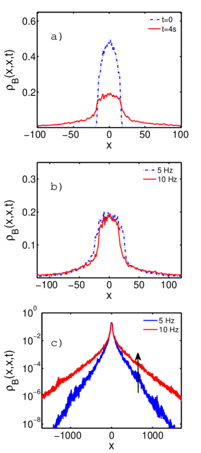
Figure 1: (color online) Anderson localization in a Tonks-Girardeau gas in dependence of the initial trap parameter $\nu$ (i.e., $\omega$). The parameters of the disordered potential are ($\sigma=0.13$ and $V_{0}=0.465$). (a) The averaged density of the Tonks-Girardeau wavepacket at $t=0$ and after $t=1450$ (=$4$ s) of propagation. The initial state corresponds to $\nu=8.67\times 10^{-2}$ ($\omega=10$ Hz). (b) Shown is the density of a Tonks-Girardeau gas (in the localized steady state) after $t=1450$ (=$4$ s) of propagation in a disordered potential. Blue dot-dashed line corresponds to $\nu=4.34\times 10^{-2}$ ($\omega=5$ Hz), whereas red solid line corresponds to $\nu=8.67\times 10^{-2}$ ($\omega=10$ Hz). (c) Same as figure (b) on a logarithmic scale. Blue line corresponds to ($\omega=5$ Hz), and red line corresponds to $\omega=10$ Hz; arrow indicates the increase of $\omega$. For $|x|$ larger than some value (call it $L_{t}$), the density decays exponentially, which characterizes Anderson localization. The density-tails decay slower for larger initial trap parameter $\omega$ (see text for details).

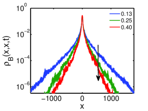
Figure 2: (color online) Anderson localization in a Tonks-Girardeau gas in dependence of the disorder parameter $\sigma$. The averaged density of a Tonks-Girardeau gas after $t=1450$ (=$4$ s) of propagation in the disordered potential. The plots correspond to $\sigma=0.13$ (blue line), $\sigma=0.25$ (green line), and $\sigma=0.40$ (red line); arrow indicates the increase of $\sigma$. The initial state corresponds to $\omega=10$ Hz, while the amplitude of the disordered potential is $V_{0}\approx 0.47$ (see text for details).

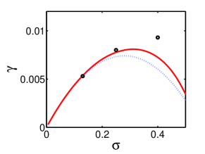
Figure 3: (color online) The exponential decay rates $\gamma^{(2)}$ (dotted blue line) and $\gamma^{(2)}+\gamma^{(3)}$ (solid red line), obtained with perturbation theory Lugan2009 , in dependence of the correlation length of the potential $\sigma$. Circles represent decay rates obtained numerically. The initial trap parameter is $\omega=10$ Hz (see text for details).

The asymptotic steady state of the system depends on the parameters of the disordered potential $\sigma$ and $V_{0}$, and on the initial state, that is, the harmonic trap parameter $\nu$. In fact, since the dynamics of the Tonks-Girardeau gas is governed by a set of uncoupled Schrödinger equations, it follows from the simple scaling of units outlined below Eq. (1), that there are in fact only two independent parameters; thus we investigate the dynamics in dependence of $\nu$ and $\sigma$, and keep $V_{0}$ at an approximately constant value. We have performed our numerical simulations in a region of the parameter space which was accessible with our numerical capabilities, but which is relevant to experiments Billy2008 ; Roati2008 . We have varied the correlation length $\sigma$ of the potential from $0.13$ up to $0.40$ (corresponding to $0.13\ \mu$m and $0.40\ \mu$m since the spatial scale is chosen to be $X_{0}=1\ \mu$m), and the harmonic trap parameters in the interval $\nu=4.34-8.67\times 10^{-2}$ (corresponding to $\omega=5-10$ Hz). The number of particles used in our simulations is relatively small, $N=13$, due to the computer limitations, however, despite of this, one can use our simulations to infer general conclusions that would be valid in an experiment with larger $N$. It should be emphasized that all plots of densities and correlations are ensemble averages made over 40 realizations of the disordered potentials.

First we investigate the behavior of the single-particle density. In Figure 1 we show $\rho_{B}(x,x,t=1450)$ versus $x$ for $(\sigma,V_{0})=(0.13,0.465)$, and two values of $\nu$: $\nu=4.34\times 10^{-2}$ ($\omega=5$ Hz) and $\nu=8.67\times 10^{-2}$ ($\omega=10$ Hz). In Fig. 1(a) we compare the initial density (at $t=0$), with the density at time $t=1450$ ($=4$ s), at which the steady state regime is already achieved (all graphs below which describe the steady state are also calculated at this time). We observe that the steady-state density has a broad central part with a fairly flat top, and decaying tails on its sides. The central part is composed of many single-particle states $\psi_{j}$. In Fig. 1(b) we plot the steady state density for two values of $\omega$. For $\omega=5$ Hz, the central part is broader than for $\omega=10$ Hz, but the tails are decaying faster with the increase of $|x|$, as shown in Fig. 1(c), where the densities are plotted in the logarithmic scale. We clearly see that for $|x|$ larger than some value (call it $L_{t}$), the density decays exponentially, which indicates Anderson localization. We have fitted the tails to the exponential curve $\rho_{B}(x,x,t)\propto\exp(-\Lambda|x|)$ and obtained $\Lambda=0.0097$ for $\omega=5$ Hz, and $\Lambda=0.0053$ for $\omega=10$ Hz, that is, we find that the density-tails decay slower for larger initial trap parameter $\omega$. For larger values of $\omega$, the trap is tighter and the initial state has larger energy and broader momentum distribution, therefore, it is harder to achieve localization of the wave packet (e.g., see Sanchez-Palencia2007 ; Lugan2009 ). Another way to interpret these simulations is in terms of the spatial correlation distance of the wave packet. An incoherent wave packet can be characterized by using the spatial correlation distance, which determines a spatial degree of coherence; this quantity is inversely proportional to the width of the spatial power spectrum. If the spatial correlation distance decreases, it is harder to achieve localization.

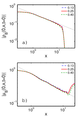
Figure 4: (color online) First-order correlations in the initial state decay algebraically. Shown are the single-particle density matrix $|\rho_{B}(0,x,0)|$ (a), and the degree of first-order coherence $|\mu_{B}(0,x,0)|$ (b), at $t=0$ for the initial state corresponding to $\omega=10$ Hz. The graphs are plotted for three values of $\sigma$ as indicated in the legend. Black dotted lines depict the fitted curves $|\rho_{B}(0,x,0)|\sim|x|^{-0.54}$ and $|\mu_{B}(0,x,0)|\sim|x|^{-0.51}$.

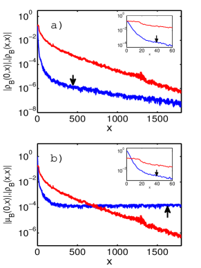
Figure 5: (color online) Correlations in the steady (Anderson localized) state. The single-particle density matrix $|\rho_{B}(0,x,t)|$ [blue line in (a), indicated with the arrow], and the degree of first order coherence $|\mu_{B}(0,x,t)|$ [blue line in (b), indicated with the arrow], at the time $4$ s. The parameters used are $\sigma=0.13$ and $\omega=10$ Hz. Red lines (in both panels) depict the single particle density $\rho_{B}(x,x,t)$. Insets enlarge the region where $|x|$ is small and where correlations decay approximately exponentially. For $|x|$ in the region of the density tails ($|x|>L_{t}$), $|\mu_{B}(0,x,t)|$ reaches a plateau. See text for details.

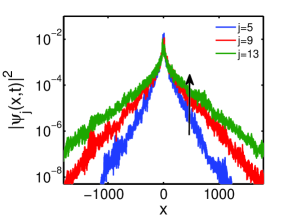
Figure 6: (color online) The single-particle states $|\psi_{j}(x,t)|^{2}$ for $j=5,9$, and $13$ in the (Anderson localized) steady state. The arrow indicates increase of $j$. The parameters used are $\sigma=0.13$ and $\omega=10$ Hz. The single-particle states for larger $j$ (larger in energy) decay slower with the increase of $|x|$. See text for details.

In Fig. 2 we display dependence of the density $\rho_{B}(x,x,t)$ versus $x$ for $\nu=8.67\times 10^{-2}$ ($\omega=10$ Hz), and three values of $(\sigma,V_{0})$: $(0.13,0.465)$, $(0.25,0.478)$, and $(0.40,0.485)$. Note that $V_{0}$ can be regarded as a constant close to $0.47$ and we will omit to explicitly write the values of $V_{0}$ besides $\sigma$ in further text; the variations of $V_{0}$ are a consequence of the method utilized to construct the random potential. We observe that the exponential tails decay faster for larger values of $\sigma$.

In order to underpin our observations we compare our numerical results to the predictions of the formalism presented in Refs. Sanchez-Palencia2007 ; Lugan2009 , which has been used to study Anderson localization of a Bose-Einstein condensate. In the approach of Ref. Sanchez-Palencia2007 , the wave packet is considered to be a superposition of almost independent plane waves ($k$-components); the wave packet had a high momentum cut-off at the inverse healing length (of the condensate). The assumption that the $k$-components are almost independent means that we should be able to employ this formalism here as well, despite of the fact that our wave packet is only partially coherent (that is, it is in the Tonks-Girardeau regime, rather than being condensed). However, for our wave packets, the momentum distribution does not have a clear cut-off but rather decays smoothly to zero as $k\rightarrow\infty$, and we must adopt a somewhat different procedure to determine the decay rate of the whole wave packet from the decay rate of the $k$-components. Within the formalism Sanchez-Palencia2007 ; Lugan2009 , the exponential decay-rate of every $k$-component is calculated by using perturbation theory, and the decay rate $\gamma(k)$ is given as a series $\gamma(k)=\sum_{n\geq 2}\gamma^{(n)}$ in increasing orders Lugan2009 . The leading contribution $\gamma^{(2)}$ to the decay rate $\gamma(k)$ arises from the Born approximation, wherein Sanchez-Palencia2007 ; Lugan2009 ; notation

$$\gamma^{(2)}(k)=\frac{\pi}{4}\left(\frac{V_{0}}{k}\right)^{2}\sigma(1-k\,\sigma)$$ (12)

for $k<\sigma^{-1}$, and zero otherwise; the next order term is given in the Appendix, see also Lugan2009 . In order to evaluate the decay rate of the expanding wave packet from $\gamma(k)$ we adopt the following simple procedure. We assume that there is an effective high momentum cut-off $k_{hmc}$, which we evaluate as follows: For the initial wave packets (determined by the trap frequency), we have numerically calculated the Lyapunov exponents $\Lambda$ determining localization. For the potential parameter $\sigma=0.13$ ($V_{0}=0.465$), and the initial condition corresponding to $\omega=10$ Hz (for these parameters the system is close to the Born approximation regime Sanchez-Palencia2007 ), we choose the effective high momentum cut off $k_{hmc}$ such that it fits the numerically calculated decay rate, that is we extract $k_{hmc}$ from the equation $\Lambda=\gamma(k_{hmc})$; this yields $k_{hmc}=1.79$. Then, by using this value, we calculate the Lyapunov exponents $\gamma(k_{hmc})$ in dependence of $\sigma$. In Fig. 3 we illustrate the functional dependence $\gamma(k_{hmc})$ vs. $\sigma$; dotted blue line depicts the Born approximation $\gamma^{(2)}$, and solid red line depicts $\gamma^{(2)}+\gamma^{(3)}$. We see that within the parameter regime studied here the trend is well described with the perturbation approach. Quantitative deviations occur because higher order terms of the perturbation theory are not negligible and should be taken into account.

Next we focus on correlations contained within the reduced single-particle density matrix $\rho_{B}(x,y,t)$. Suppose that we are interested in the phase correlations between the center (at zero) and the rest of the cloud (at some $x$-value); the quantity $\rho_{B}(0,x,t)$ will decay to zero with the increase of $|x|$ even if the field is perfectly coherent simply because the density decays to zero on the tails. In order to extract solely correlations from the RSPDM, we observe the behavior of the quantity Naraschewski1999

$$\mu_{B}(x,y,t)=\frac{\rho_{B}(x,y,t)}{\sqrt{\rho_{B}(x,x,t)\rho_{B}(y,y,t)}},$$ (13)

which is the degree of first-order coherence Naraschewski1999 (in optics it is sometimes referred to as the complex coherence factor MandelWolf ). In the context of ultracold gases $\mu_{B}(x,y,t)$ can be interpreted as follows: If two narrow slits were made at points $x$ and $y$ of the 1D Tonks-Girardeau gas, and if the gas was allowed to drop from these slits, expand and interfere, $\mu_{B}(x,y,t)$ expresses the modulation depth of the interference fringes. In this work we investigate correlations between the central point of the wave packet and the tails: $\mu_{B}(0,x,t)$.

In Fig. 4 we show the averages of the magnitudes of the one-body density matrix $|\rho_{B}(0,x,t)|$, and the degree of first order coherence $|\mu_{B}(0,x,t)|$, at time $t=0$ for the initial state corresponding to $\omega=10$ Hz and for three values of $\sigma$. From previous studies of the harmonic potential ground-state (e.g., see Ref. Forrester2003 for the continuous Tonks-Girardeau gas and Rigol2005 for hard-core bosons on the lattice) it follows that in a fairly broad interval of $x$-values, both $|\rho_{B}(0,x,t=0)|$ and $|\mu_{B}(0,x,t=0)|$ decay approximately as a power law $|x|^{-\gamma_{0}}$ with the exponent $\gamma_{0}=0.5$ Forrester2003 ; Rigol2005 , despite of the fact that the density is not homogeneous; the density dependent factors multiplying the power law are also known Forrester2003 ; Rigol2005 . We have observed that the initial correlation functions are well fitted to the power law: $|\rho_{B}(0,x,0)|\sim|x|^{-0.54}$ and $|\mu_{B}(0,x,0)|\sim|x|^{-0.51}$ for $\omega=10$ Hz (for $\omega=5$ Hz, we obtain $|\rho_{B}(0,x,0)|\sim|x|^{-0.60}$ and $|\mu_{B}(0,x,0)|\sim|x|^{-0.55}$). The power-law decay of correlations indicates presence of quasi long-range order. Apparently, the properties of the small random potential do not significantly affect the correlations of the initial state for the trap strengths $\omega$, and disorder parameters used in our simulations. This happens because the initial single particle states are localized by the trapping potential, rather than by disorder (their decay is Gaussian). The effect of disorder on these states becomes more significant for weaker traps, because the disordered potential becomes nonegligible in comparison to the harmonic term $\nu^{2}x^{2}$ in a broader region of space. In fact, we expect that if one keeps the number of particles constant, for sufficiently shallow traps, disorder would qualitatively change the behavior of the correlations in the initial state, in a similar fashion as when the trap is absent. However, probing Anderson localization by using transport (i.e., expansion of an initially localized wave packet), is perhaps more meaningful for tighter initial traps, where the initial wave packets are localized by the trap rather than by disorder.

For very small values of $|x|$, and for very large values (at the very tails of the wave packet) there are deviations from the power law behavior Forrester2003 ; Rigol2005 . The behavior of $|\mu_{B}(0,x,0)|$ at the tails, where $|\mu_{B}(0,x,0)|$ starts to grow up to some constant value is attributed to the fact that higher single-particle states $\psi_{m}(x,0)$ decay at a slower rate with the increase of $|x|$, and therefore spatial coherence increases in the tails (see also the discussion below).

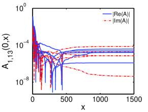
Figure 7: (color online) The absolute value of the real and imaginary part of $A_{ij}(0,x,t)$ for $i=1$ and $j=13$, and five different realizations of the disordered potential. The parameters used in the simulation are $\sigma=0.13$ and $\omega=10$ Hz. For sufficiently large $|x|$, $A_{ij}(0,x,t)$ reaches a constant value. See text for details.

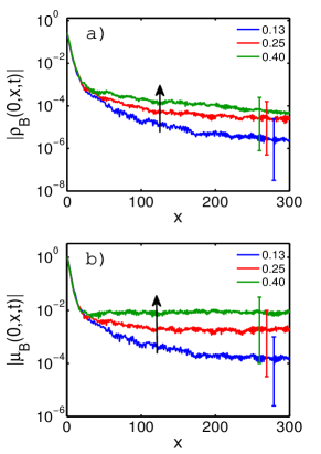
Figure 8: (color online) Correlations in the steady (Anderson localized) state in dependence of the disorder parameter $\sigma$. Shown are the correlations at $t=1450$ ($=4$ s) for $\sigma=0.13$, $0.25,$ and $0.40$. The arrows indicate increase of $\sigma$, whereas the vertical bars indicate the uncertainty in correlations at the plateau values. For a given set of parameters $\sigma$ and $\omega$, $90\%$ of the simulations (one simulation is made for a single realization of $V_{D}$) fall within the vertical bars. The initial trap parameter is $\omega=10$ Hz. See text for details.

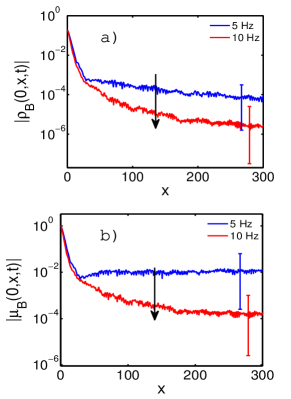
Figure 9: (color online) Correlations in the steady state in dependence of the initial trap parameter $\omega$. Shown are the correlations at $t=1450$ ($4$ s) for two initial conditions corresponding to $\omega=5$ Hz and $10$ Hz. The arrows indicate the increase of $\omega$, whereas the vertical bars indicate the uncertainty in correlations at the plateau values. Other parameters are identical as in Fig. 1.

After the Tonks-Girardeau gas expands in the disordered potential and reaches a steady-state, the behavior of $\rho_{B}(0,x,t)$ and $\mu_{B}(0,x,t)$ significantly differs from that at $t=0$. This is shown in Fig. 5, where we display the magnitude of the two functions for $\sigma=0.13$ and $\omega=10$ Hz. We observe that $|\rho_{B}(0,x,t)|$ exhibits a fairly fast exponential decay for small values of $|x|$, that is, in the region where the density is relatively large [see the inset in Fig. 5(a)]. This fast decay slows down up to sufficiently large values of $x$, i.e., $|x|>L_{t}$, where we observe slower exponential decay of $|\rho_{B}(0,x,t)|$, which corresponds to the exponentially decaying tails in the single-particle density of the localized steady state. Regarding the degree of first-order coherence $|\mu_{B}(0,x,t)|$, we find that for sufficiently small $|x|$, it decays exponentially [see the inset in Fig. 5(b)]; however, as $x$ approaches the region of exponentially decaying tails $|x|>L_{t}$, the exponential decay of $|\mu_{B}(0,x,t)|$ slows down until it reaches roughly a constant value in the region $|x|>L_{t}$. This plateau occurs because single-particle states $\psi_{j}$ decay slower for larger $j$ values (they are higher in energy and momentum), and due to the fact that for sufficiently large $|x|$, the matrix elements $A_{ij}(0,x,t)$, which are important ingredients in expression (6) for $|\rho_{B}(0,x,t)|$, also reach a constant value. This is depicted in Figs. 6 and 7, which display $|\psi_{j}(x,t)|^{2}$ for $j=5,9$, and $13$, and $A_{1,13}(0,x,t)$ (real and imaginary part) for five different realizations of the disordered potential. We clearly see that $A_{ij}(0,x,t)$ reaches a constant value (generally complex off the diagonal), which differs from one realization of the disorder to the next; this is connected to the fact that the integral $\int_{0}^{x}dx^{\prime}\psi_{i}^{*}(x^{\prime},t)\psi_{j}(x^{\prime},t)$ converges to a constant value for sufficiently large $x$, which is a consequence of the exponential localization. The fluctuations in $A_{ij}(0,x,t)$ are reflected onto the fluctuations of the plateau value of $|\mu_{B}(0,x,t)|$. We have compared the averages of the matrix elements $A_{ij}(0,x,t)$ for large $x$ (at the plateau) for all values of $i$ and $j$. They are all within one order of magnitude with $A_{13,13}(0,x,t)$ ($N=13$) being the largest, more specifically, the averages of some of the absolute value in our simulations are $|A_{13,13}(0,x,t)|=0.25\times 10^{-3}$, $|A_{7,7}(0,x,t)|=0.16\times 10^{-3}$, $|A_{1,1}(0,x,t)|=0.06\times 10^{-3}$, and $|A_{1,13}(0,x,t)|=0.03\times 10^{-3}$. Thus, the values of the matrix elements to some extent enhance the contribution of the highest single-particle states in the correlations $|\mu(0,x,t)|$. It is worthy to mention that identical effect is observed in incoherent light solitons (e.g., see IncOpt ), where the coherence also increases in the tails, which is observed in the complex coherence factor in optics (in the case of solitons, it is nonlinearity, rather than disorder which keeps the wave packet localized).

Figure 8 displays the correlations for three values of $\sigma$ ($\sigma=0.13$, $0.25$, and $0.40$). In the parameter regime that we investigated, we found no clear dependence of $|\rho_{B}(0,x,t)|$ and $|\mu_{B}(0,x,t)|$ (in the steady state at $4$ s) on $\sigma$ for small values of $|x|$. For $|x|$ in the region of the tails, $|x|>L_{t}$, the correlations $|\mu_{B}(0,x,t)|$ asymptote larger values for larger $\sigma$. All of the qualitative observations above were made throughout the parameter regime that we investigated numerically.

In Figure 9 we display $|\rho_{B}(0,x,t)|$ and $|\mu_{B}(0,x,t)|$, for two different initial conditions corresponding to $\omega=5$ Hz and $10$ Hz; other parameters are identical as in Fig. 1, that is, $\sigma=0.13$. We have observed that for asymptotic values of $t$, the magnitude of correlations $|\mu_{B}(0,x,t)|$ is lower for larger values of $\omega$. It is worthy to mention that a plateau in $|\mu_{B}(0,x,t)|$ occurs in every numerical simulation for a given realization of the disordered potential, but in every realization on a somewhat different value; the vertical bars in Figs. 8 and 9 indicate a spread in plateau values in our simulations.

If we compare Fig. 8 with Fig. 2, and Fig. 9 with Fig. 1 (compare the direction of arrows in corresponding figures), one finds that if the density in the tails decays faster, the correlations between the center of the cloud and the tails decrease slower. This is in agreement with our interpretation that a slower decay (with $|x|$) of higher single-particle states $\psi_{j}$ (see Fig. 6) is responsible for the creation of plateaus in $|\mu(0,x,t)|$ and increase of coherence in the tails; namely, if the density decays faster (with $|x|$), the highest single particle state $\psi_{N}$ will become dominant for smaller values of $x$ leading to greater coherence in $|\mu(0,x,t)|$.

Let us now extrapolate our numerical calculations and results to larger particle numbers. Suppose that we keep all parameters fixed, and increase only $N$. The energy of the initial state as well as the high momentum cut-off $k_{hcm}$ increase with the increase of $N$. Our simulations up to a finite time up of $4$ s would not be able to see exponentially decaying tails of the asymptotic steady state. By employing the results of Ref. Lugan2009 , one concludes that the steady state will always be localized, however, at larger values of $N$, the Born-approximation mobility edge Lugan2009 will be crossed and the exponents describing the exponentially decaying tails will be smaller. The plateaus in the correlations will still exist in the regions of these tails, however, the value $|\mu_{B}(0,x,t)|$ will decrease with the increase of $N$ (simply because more single particle states $\psi_{j}$ are needed to describe the Tonks-Girardeau state), and both the exponentially decaying tails together with the plateaus will be harder to observe. The effect where the coherence of the localized steady state increases in the tails should however be observable also with partially condensed BECs, below the Tonks-Girardeau regime.

IV Conclusion

We have investigated Anderson localization of a Tonks-Girardeau gas in continuous potentials [$V_{D}(x)$] with controlled disorder, by investigating expansion of the gas in such potentials; for the initial state we have chosen the Tonks-Girardeau ground state in a harmonic trap (with $V_{D}(x)$ superimposed upon it), and we have analyzed the properties of the (asymptotic) steady state obtained dynamically. We have studied the dependence of the Lyapunov exponents and correlations on the initial trap parameter $\omega$ [$5-10$ Hz], and the correlation length of the disorder $\sigma$ [$0.13-0.40$ $\mu$m]. We found that the Lyapunov exponents of the steady state, decrease with the increase of $\nu$. In the parameter regime considered the Lyapunov exponents increased with the increase of $\sigma$, which was underpinned by the perturbation theory. The behavior of the correlations contained in the one-body density matrix $\rho_{B}(x,y,t)$ and the degree of first order coherence indicate that the off diagonal correlations $|\rho_{B}(0,x,t)|$ decrease exponentially with the increase of $|x|$, due to the exponential decay of the density, however, in the region of the exponentially decaying tails, the degree of first-order coherence $|\mu_{B}(0,x,t)|$ reaches a plateau. This is connected to the behavior of the single-particle states used to construct the Tonks-Girardeau wave function and to the increase of coherence in the exponentially decaying tails. This effect is analogous to the one found in incoherent optical solitons, for which coherence also increases in the tails.

As a possible direction for further research we envision a study of Anderson localization for incoherent light in disordered potentials, Anderson localization within the framework of the Lieb-Liniger model describing a 1D Bose gas with finite strength interactions (which becomes identical to the Tonks-Girardeau model when the interaction strength becomes infinite). These studies should provide further insight into the influence of wave coherence (within the context of optics), and the influence of interactions on Anderson localization (within the context of effectively 1D ultracold atomic gases).

Appendix A Construction of the disordered potential

In this section we describe the numerical procedure utilized for construction of the disordered potential $V_{D}(x)$. The $x$-space is numerically simulated by using 33000 equidistant points in the interval $x\in[-2000,2000]$. From this array, we have constructed a random array $v=\exp[2\pi\,\mbox{rand}(x)i]$ of the same length, where $\mbox{rand}(x)$ denotes a random number in between $0$ and $1$. Then we calculated a discrete Fourier transform of $v$ (call it $\tilde{v}(k)$), and introduced a cut-off wave vector $K_{cut}$. $V_{D}(x)$ was chosen to be an absolute value of the inverse discrete Fourier transform of $\tilde{v}(k)\Theta(2k/K_{cut})$ [where $\Theta(x)$ is one for $|x|<1$ and zero otherwise]. We have calculated the autocorrelation function $A_{C}(x)$ of the potential and fitted it to the functional form $\sin(x/\sigma)/(x/\sigma)^{2}$ to get the correlation length $\sigma$. The autocorrelation function $A_{C}(x)$ of the disordered potential $V_{D}(x)$ is identical to the autocorrelation function of the potential used in the experiment of Ref. Billy2008 , and the theoretical studies conducted in Refs. Sanchez-Palencia2007 ; Lugan2009 . The higher order correlators differ, but they do not qualitatively change any conclusions in the parameter regime studied here.

Let us define the term $\gamma^{(3)}(k)$ which is used in the series $\gamma(k)=\sum_{n\geq 2}\gamma^{(n)}$ (see Ref. Lugan2009 and Fig. 3). This term depends on the 3-point correlator of the random potential Lugan2009 :

$$c_{3}(\frac{x_{1}}{\sigma},\frac{x_{2}}{\sigma})=\frac{1}{V_{0}^{3}}\ \langle\overline{V}_{D}(x^{\prime}-x_{1})\overline{V}_{D}(x^{\prime}-x_{2})\overline{V}_{D}(x^{\prime})\rangle_{x^{\prime}},$$ (14)

and it is given by:

$$\gamma^{(3)}(k)=\frac{2{V_{0}}^{3}\sigma^{2}}{k^{3}}f_{3}(k\sigma),$$ (15)

where $f_{3}(\kappa)$ is defined as:

$$f_{3}(\kappa)=-\frac{1}{4}\int^{0}_{-\infty}\,\!\!du\int^{u}_{-\infty}dv\ c_{3}(u,v)\sin(2\kappa v)\ .$$ (16)

The 3-point correlator was calculated numerically to obtain Fig. 3.

References

- (1) P.W. Anderson, Phys. Rev. 109, 1492 (1958).
- (2) D.S. Wiersma, P. Bartolini, A. Lagendijk, R. Righini, Nature 390, 671 (1997).
- (3) A.A. Chabanov, M. Stoytchev, A.Z. Genack, Nature 404, 850 (2000).
- (4) M. Störzer, P. Gross, C.M. Aegerter, G. Maret, Phys. Rev. Lett. 96, 063904 (2006).
- (5) T. Schwartz, G. Bartal, S. Fishman, and M. Segev, Nature 446, 52 (2007).
- (6) Y. Lahini, A. Avidan, F. Pozzi, M. Sorel, R. Morandotti, D.N. Christodoulides, and Y. Silberberg, Phys. Rev. Lett. 100, 013906 (2008).
- (7) J. Billy, V. Josse, Z. Zuo, A. Bernard, B. Hambrecht, P. Lugan, D. Clement, L. Sanchez-Palencia, P. Bouyer, A. Aspect, Nature 453, 891 (2008).
- (8) G. Roati, C. D’Errico, L. Fallani, M. Fattori, C. Fort, M. Zaccanti, G. Modugno, M. Modugno, M. Inguscio, Nature 453, 895 (2008).
- (9) L. Sanchez-Palencia and M. Lewenstein, Nature Phys. 6, 87 (2010).
- (10) M. Girardeau, J. Math. Phys. 1, 516 (1960).
- (11) M. Girardeau and E.M. Wright, Phys. Rev. Lett. 84, 5691 (2000).
- (12) M. Olshanii, Phys. Rev. Lett. 81, 938 (1998).
- (13) D.S. Petrov, G.V. Shlyapnikov, and J.T.M. Walraven, Phys. Rev. Lett. 85 3745 (2000).
- (14) V. Dunjko, V. Lorent, and M. Olshanii, Phys. Rev. Lett. 86 5413 (2001).
- (15) T. Kinoshita, T. Wenger, and D.S. Weiss, Science 305, 1125 (2004).
- (16) B. Paredes, A. Widera, V. Murg, O. Mandel, S. Fölling, I. Cirac, G. V. Shlyapnikov, T. W. Hänsch, and I. Bloch, Nature (London) 429, 277 (2004).
- (17) T. Kinoshita, T. Wenger, and D.S. Weiss, Nature (London) 440, 900 (2006).
- (18) A. Lenard, J. Math. Phys. 5, 930 (1964).
- (19) P.J. Forrester, N.E. Frankel, T.M. Garoni, and N.S. Witte, Phys. Rev. A 67, 043607 (2003); T. Papenbrock, Phys. Rev. A 67, 041601 (2003).
- (20) M. Rigol and A. Muramatsu, Phys. Rev. Lett 94, 240403 (2005).
- (21) A. Minguzzi and D.M. Gangardt, Phys. Rev. Lett. 94, 240404 (2005).
- (22) A. del Campo and J.G. Muga, Europhys. Lett. 74, 965 (2006).
- (23) D.M. Gangardt and M. Pustilnik, Phys. Rev. A 77, 041604(R) (2008).
- (24) B. Damski, J. Zakrzewski, L. Santos, P. Zoller, and M. Lewenstein, Phys. Rev. Lett. 91, 080403 (2003).
- (25) R. Roth and K. Burnett, Phys. Rev. A 68, 023604 (2003).
- (26) L. Sanchez-Palencia, D. Clement, P. Lugan, P. Bouyer, G.V. Shlyapnikov, and A. Aspect, Phys. Rev. Lett. 98, 210401 (2007).
- (27) T. Giamarchi and H.J. Schulz, Phys. Rev. B 37, 325 (1988).
- (28) M.P.A. Fisher, P.B. Weichman, G. Grinstein, and D.S. Fisher, Phys. Rev. B 40, 546 (1989).
- (29) H. Gimperlein, S. Wessel, J. Schmiedmayer, and L. Santos, Phys. Rev. Lett. 95, 170401 (2005).
- (30) A. De Martino, M. Thorwart, R. Egger, and R. Graham, Phys. Rev. Lett. 94, 060402 (2005).
- (31) V.W. Scarola and S. Das Sarma, Phys. Rev. A 73, 041609(R) (2006).
- (32) A.M. Rey, I.I. Satija, and C.W. Clark, Phys. Rev. A 73, 063610 (2006).
- (33) B. Horstmann, J.I. Cirac, and T. Roscilde, Phys. Rev. A 76, 043625 (2007).
- (34) G. Roux, T. Barthel, I.P. McCulloch, C. Kollath, U. Schollwöck, and T. Giamarchi, Phys. Rev. A 78, 023628 (2008).
- (35) X. Deng, R. Citro, A. Minguzzi, and E. Orignac, Phys. Rev. A, 78, 013625 (2008).
- (36) T. Roscilde, Phys. Rev. A 77, 063605 (2008).
- (37) G. Orso, A. Iucci, M.A. Cazalilla, and T. Giamarchi, Phys. Rev. A 80, 033625 (2009).
- (38) M. Rigol and A. Muramatsu, Phys. Rev. A 72, 013604 (2005); ibid., 70, 031603 (2004).
- (39) M. Mitchell, M. Segev, T.H. Coskun, and D.N. Christodoulides, Phys. Rev. Lett. 79, 4990 (1997); M.I. Carvalho, T.H. Coskun, D.N. Christodoulides, M. Mitchell, and M. Segev, Phys. Rev. E 59, 1193 (1999); H. Buljan, T. Schwartz, M. Segev, M. Soljačić, and D.N. Christodoulides, J. Opt. Soc. Am. B 21, 397 (2004).
- (40) H. Buljan, O. Manela, R. Pezer, A. Vardi, and M. Segev, Phys. Rev. A 74, 043610 (2006).
- (41) R. Pezer and H. Buljan, Phys. Rev. Lett. 98, 240403 (2007).
- (42) P. Lugan, A. Aspect, and L. Sanchez-Palencia, D. Delande, B. Gremaud, C.A. Müller, C. Miniatura, Phys. Rev. A 80, 023605 (2009).
- (43) We utilize notation from Ref. Lugan2009 to denote the orders of the perturbation, however, the coefficients here describe the decay of density, rather than the wave function as in Lugan2009 , and they differ by a factor of .
- (44) M. Naraschewski and R.J. Glauber, Phys. Rev. A 59, 4595 (1999).
- (45) L. Mandel and E. Wolf, Optical Coherence and Quantum Optics (Cambridge Press, New York, 1995).