A Sample of Intermediate-Mass Star-Forming Regions: Making Stars at Mass Column Densities $<$1 g cm^-2

Abstract

In an effort to understand the factors that govern the transition from low- to high-mass star formation, we identify for the first time a sample of intermediate-mass star-forming regions (IM SFRs) where stars up to—but not exceeding—$\sim 8$ M_☉ are being produced. We use IRAS colors and Spitzer Space Telescope mid-IR images, in conjunction with millimeter continuum and ¹³CO maps, to compile a sample of 50 IM SFRs in the inner Galaxy. These are likely to be precursors to Herbig AeBe stars and their associated clusters of low-mass stars. IM SFRs constitute embedded clusters at an early evolutionary stage akin to compact H II regions, but they lack the massive ionizing central star(s). The photodissociation regions that demarcate IM SFRs have typical diameters of $\sim 1$ pc and luminosities of $\sim 10^{4}$ L_☉, making them an order of magnitude less luminous than (ultra)compact H II regions. IM SFRs coincide with molecular clumps of mass $\sim 10^{3}$ M_☉ which, in turn, lie within larger molecular clouds spanning the lower end of the giant molecular cloud mass range, $10^{4}-10^{5}$ M_☉. The IR luminosity and associated molecular mass of IM SFRs are correlated, consistent with the known luminosity–mass relationship of compact H II regions. Peak mass column densities within IM SFRs are $\sim$ 0.1–0.5 g cm^-2, a factor of several lower than ultra-compact H II regions, supporting the proposition that there is a threshold for massive star formation at $\sim$ 1 g cm^-2.

1 Introduction

It has become clear that high-mass star formation cannot be viewed simply as a scaled-up version of the low-mass star formation paradigm (Zinnecker & Yorke, 2007). High-mass ($M>8$ M_☉) and low-mass ($M<2$ M_☉) star formation seem to require some fundamentally different conditions and physical processes that probably involve differences in turbulence and magnetic fields within their formative clouds as much as differences in cloud mass and density (Krumholz & McKee, 2005). Stars forming in the 2 to 8 solar mass range (intermediate-mass; IM) are especially interesting as they straddle the boundary between the low- and high-mass paradigms and can provide a window into the processes that govern the transition from low-mass to high-mass star formation. Extensive studies of these IM star-forming regions (IM SFRs), i.e., SFRs where the most massive star is IM, have not been possible in the past due to difficulties in clearly identifying the regions and the lack of angular resolution to investigate them in detail.

Our goals in this investigation of intermediate-mass star-forming regions are to understand what controls or enables the transition from low- to high-mass star formation. Is it simply a question of an enhanced reservoir of material that promotes the formation of a more massive star, or is star formation shut off in some cases because of disruption of the parent molecular cloud? Is there evidence for sequential or triggered star formation in the interstellar medium (ISM) surrounding IM SFRs as around massive SFRs (Deharveng et al., 2005)? How common are bipolar outflows? What is the ISM environment of these regions? Are IM SFRs found in locations where high-mass star formation is also occurring or in relative isolation? What are the typical masses and velocity dispersions of IM star-forming clouds? What are the typical sizes and luminosities of IM SFRs?

The aim of the present paper, the first high-resolution study of IM SFRs, is to determine some basic properties of a carefully selected sample of IM SFRs. We present our candidate selection criteria and classification in Section 2. We then, in Section 3, identify CO features corresponding to the candidates and discuss a particularly interesting sample of the candidates. The photometry and spectral energy distribution is examined in Section 4, and the molecular material is discussed in Section 5. We compare our sample to Ultra-Compact H II (UCH II) regions in Section 6. Finally, we present a discussion in Section 7 and conclusions in Section 8.

2 Infrared Analysis

2.1 Defining a Sample of Candidate IM SFRs

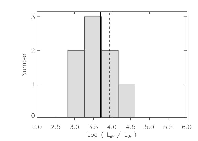
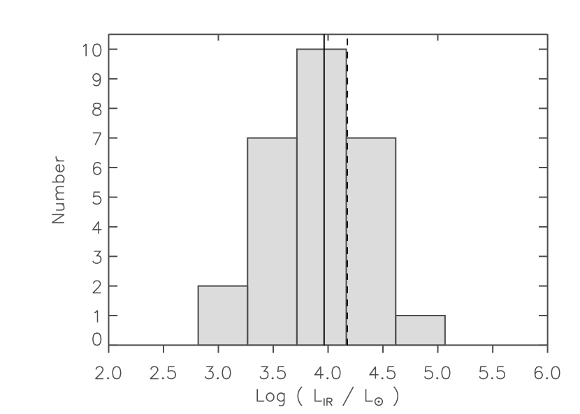
Figure 12: (Left) Histogram of $\log(L_{\mathrm{IR}}/L_{\sun})$ for the eight near IM SFRs. The solid line represents $\log(\mathrm{median})=3.7$ while the dashed line represents $\log(\mathrm{average})=3.9$. (Right) Histogram of $\log(L_{\mathrm{IR}}/L_{\sun})$ for the 27 IM SFRs that have assigned distances. The solid line represents $\log(\mathrm{median})=4.0$ while the dashed line represents $\log(\mathrm{average})=4.2$. The bin size is 0.45 dex.

Kerton (2002), using 21 cm H I emission, identified a sample of IM SFRs and determined that they occupy a distinct region of the IRAS color-color diagram, see Figure 1, left panel and Figure 12 in Kerton (2002). They are separate from H II regions, and quite distinct from T Tauri and Herbig AeBe stars (Barnes & Myers, 1993; Weintraub, 1990): $-0.18<\log(F_{\nu}(25)/F_{\nu}(12))<0.40$, $0.96<\log(F_{\nu}(60)/F_{\nu}(25))<1.56$ and $0.29<\log(F_{\nu}(100)/F_{\nu}(60))<0.69$. These distinct colors arise from the combined effect of lowered dust temperatures surrounding IM stars and increased survivability of 12 $\micron$-emitting grains in the less harsh radiation environment (Giard et al., 1994). The color criteria from Kerton (2002) are probably biased toward the higher end of the intermediate mass range because the color criteria were based on objects that could produce a significant amount of H I in a photodissociation region.

We queried the IRAS Point Source Catalog v2.1 (PSC) with the above color criteria. In all cases, we required the IRAS flux density quality to be marked as either high ($F_{\mathrm{qual}}=3$) or moderate ($F_{\mathrm{qual}}=2$). Table 1 lists the results of this query over several regions of interest. Over the entire sky there are 984 sources meeting these criteria. In the region within 1 degree ($|b|<1\arcdeg$) of the Galactic Plane where most star formation takes place, there are 360 sources. In this paper, we focused on the 70 sources at Galactic longitudes between $14\arcdeg<\ell<55\fdg 7$ where complementary data from several multiwavelength Galactic surveys are available, namely the The Boston University Five College Radio Astronomy Observatory (BU-FCRAO) Galactic Ring Survey (GRS; Jackson et al., 2006) in ¹³CO, the mid-IR Galactic Legacy Infrared Mid-Plane Survey Extraordinaire I (GLIMPSE; Benjamin et al., 2003), the Multiband Infrared Photometer for Spitzer Galactic survey I (MIPSGAL; Carey et al., 2005) and the Bolocam Galactic Plane Survey (BGPS; Aguirre et al., 2009). Out of the 70 IRAS sources, 66 fall within the fully covered GRS field ($18\arcdeg<\ell<55\fdg 7$), and 4 objects fall within the partially covered part of the GRS ($14\arcdeg<\ell<18\arcdeg$).

Use of the IRAS PSC to define our baseline sample of IM SFRs likely results in a small bias against very nearby sources which would have angular sizes larger than the IRAS beam. The IRAS PSC contains objects with angular sizes of less than $0.5\arcmin$, $0.5\arcmin$, $1\arcmin$, and $2\arcmin$ in the scan direction for 12, 25, 60 and 100 $\micron$ respectively. A 1 pc diameter source is larger than $2\arcmin$ in angular size for a distance $<1720$ pc. There is an IRAS Small Scale Structure Catalog (SSSC) which contains information on structures up to $8\arcmin$ in angular extent. A search of this catalog over the whole sky for the same color criteria (but without the flux density quality criteria) returned 25 sources. Most of them are outside of the GLIMPSE/GRS region and all but one have an associated IRAS point source. Thus, we could miss close IM SFRs by using the IRAS PSC, but we are likely not missing a large population since that volume is small compared to the covered volume.

2.2 Infrared Morphological Classification with Spitzer

We investigated the 70 selected IRAS sources using images from the Spitzer GLIMPSE I and MIPSGAL I legacy surveys. The GLIMPSE I images have $\sim 2\arcsec$ resolution and $5\sigma$ sensitivities of 0.2, 0.2, 0.4, and 0.4 mJy in the Infrared Array Camera (IRAC; Fazio et al., 2004) wavebands centered near 3.6, 4.5, 5.8, and 8.0 $\micron$. For this study we used the available $6\arcsec$ resolution ($5\sigma$ sensitivity of 1.7 mJy) Multiband Infrared Photometer for Spitzer (MIPS; Rieke et al., 2004) 24 $\micron$ images from the MIPSGAL I survey. These images provide a vast improvement in angular resolution over the arcminute-scale IRAS images previously available.

Based on the GLIMPSE and MIPSGAL images, we classified by eye the 70 sources into three broad classes: “Blobs/Shells”, “Filamentary” and “Star-like”. Blobs/Shells are characterized by apparent circular or elliptical morphology, predominantly in the 8.0 and 24 $\micron$ bands. Blobs are typically circular (or elliptical) regions of extended emission having similar morphologies at 8.0 and 24 $\micron$ bands, while shells are usually ring-shaped 8.0 $\micron$ features that spatially coincide with 24 $\micron$ extended emission. Filamentary objects usually are emitting regions that occupy a small part of a larger filamentary structure, like a bead on a string. The structure of the region itself is usually dominated by the larger filament it sits on, and can even be irregular. This class also includes emitting regions located where filaments intersect. Finally, objects were classified as star-like where the emission appear to come from one or more point sources in all bands. No extended emission is evident for these objects. These star-like objects are not likely IM SFRs, since a point source diameter of $2\arcsec$ or less corresponds to a physical size of $<0.02$ pc at a distance of 2 kpc.

Out of the 70 surveyed IRAS objects, 49 ($70\%$) were classified as blobs/shells, 11 ($16\%$) as filamentary and 10 ($14\%$) as star-like. The right panel of Figure 1 shows their distribution in IRAS color-color space. The three groups show no grouping or preferential location in Figure 1. The IRAS names and positions for the filamentary and star-like objects are listed in Table 2. The 49 blobs/shells were investigated in more detail in the rest of the paper, as their morphology is most consistent with the expected morphology of an IM SFR. Table 3 lists the IRAS names, positions ($\ell$ and $b$), angular diameters ($\theta$) in arcminutes, velocity associations and widths ($V_{\mathrm{LSR}}$ and $\Delta V$, discussed in Section 3), calculated near and far distances ($d_{\mathrm{near}}$ and $d_{\mathrm{far}}$), adopted distances, flags noting what distance was adopted, and the calculated diameter in pc of the blobs and shells. Table 3 contains 50 entries because one of them, IRAS 19012+0505, has been divided into two sources (North and South), that have slightly different velocity associations.

3 Molecular Counterparts and Distances

3.1 CO Associations

We investigated the GRS CO spectral data cubes visually toward the regions of interest, the 49 objects classified as “Blobs/Shells”. This ¹³CO molecular line survey has a spectral resolution of $0.2$ km s^-1, an angular resolution of $46\arcsec$, and a sensitivity of $<0.4$ K. We searched for molecular features similar in morphology to the mid-IR blobs and shells. We found that the majority, 41 objects, have unambiguous CO associations, i.e., either a single CO spectral peak matches the candidate IM SFR, or if multiple peaks appear along the line of sight, the CO morphology for a particular peak can be matched to the mid-IR feature. The width of the morphologically matched feature in each GRS CO spectrum defines a velocity range that we used to construct the zeroth-moment map from the GRS spectral cubes. As a check of the morphological association between CO and the candidate IM SFR, the candidate was required to be spatially associated with a local maximum in the GRS zeroth-moment map. Of the remaining eight objects, seven have several possible associations in the data cube, resulting in an ambiguous radial velocity. These are labeled with the flag “A” in Table 3. The single remaining candidate, IRAS 19056+0947, was found to have no CO association at all within a radius of $0\fdg 3$. This object is labeled with the flag “No CO” and could be a reflection nebula, a known contaminant (see the left panel of Figure 1).

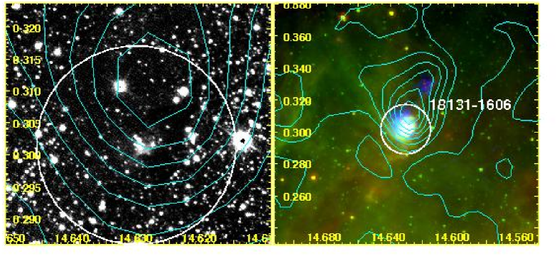
Figure 2: Four views of IRAS 18131-1606. (Top left) UKIDSS K-band image. (Top right) RGB composite of Spitzer MIPS 24 $\micron$ (red), Spitzer IRAC 8.0 $\micron$ (green), and BGPS 1.1 mm continuum (blue) images. The guiding circle shown in the two top panels has the same position and angular size and corresponds to the aperture radius of $54\arcsec$ in Table 4. The contour levels in both top panels show integrated CO intensity in the zeroth-moment map, in steps of 10%, from 90% to 10% of the peak (in this case $I_{\mathrm{peak}}=28.5$ K km s^-1, from Table 5). (Bottom left) Spectral energy distribution between 3.6–100 $\micron$. Spitzer IRAC and MIPS 24 $\micron$ flux densities are displayed as diamonds. IRAS PSC flux densities are displayed as squares. (Bottom right) The spatially averaged GRS 1-D CO spectrum, where the shaded area corresponds to the velocity range used to make the zeroth-moment map ($\Delta V$ from Table 3). IRAS 18131-1606 falls within the partially covered GRS area. It is a $1\arcmin$ blob at 8.0 and 24 $\micron$, with a possible clustering of 2.2 $\micron$ point sources at the center. The IRAS source is mentioned in Kwok et al. (1997) as having PAH features in its low resolution IRAS spectrum, which is consistent with our interpretation of the source as an IM SFR. The blob is connected through a 24 $\micron$ arc coming up from the Galactic south, connecting it to G14.6+0.1, a larger H II region (Kuchar & Clark, 1997). The blob is spatially associated with the source G014.634+00.308 from the BGPS source catalog (Rosolowsky et al., 2010). This BGPS source is clearly seen in blue.

Figure 2 shows a compilation of the basic data for the candidate IM SFR IRAS 18131-1606 (higher resolution images will be available on-line through the Astronomical Journal). The top left panel is an UKIRT Infrared Deep Sky Survey (UKIDSS; Warren et al., 2007) K-band image. The top right panel is an RGB composite of Spitzer MIPS 24 $\micron$ (red), Spitzer IRAC 8.0 $\micron$ (green), and BGPS 1.1 mm continuum (blue) images. Spitzer 8.0 $\micron$ shows the presence of polycyclic aromatic hydrocarbons (PAHs) and Spitzer 24 $\micron$ shows the presence of hot dust. The BGPS is a 1.1 mm continuum survey of the Galactic Plane with an effective resolution of $33\arcsec$ and a non-uniform $1\sigma$ noise level in the range of 30 to 60 mJy beam^-1. The BGPS shows thermal dust emission from cold, dense material. The guiding circle shown has the same position in both panels and is the same angular size (in this case the aperture radius is $54\arcsec$, from Table 4) as the aperture used to do photometry (Section 4). The contour levels in both top panels show integrated CO intensity in the zeroth-moment map, in steps of 10%, from 90% to 10% of the peak (in this case $I_{\mathrm{peak}}=28.5$ K km s^-1, from Table 5). The bottom right panel shows the spatially averaged GRS 1-D CO spectrum, where the shaded area corresponds to the velocity range used to make the zeroth-moment map ($\Delta V$ from Table 3). The bottom left panel shows the spectral energy distribution (SED, described further in Section 4) between 3.6–100 $\micron$, where Spitzer IRAC and MIPS 24 $\micron$ flux densities are displayed as diamonds, and IRAS PSC flux densities are displayed as squares.

3.2 Distances and Sizes

We estimated the LSR velocity ($V_{\mathrm{LSR}}$) of each candidate IM SFR by measuring the peak of the CO feature in a 1-D spectrum produced by averaging the GRS cube of each candidate IM SFR over the area of the mid-IR feature, typically a region covering 4–16 GRS pixels (1 GRS pixel = $22\arcsec\times 22\arcsec$). The results are shown in Table 3. Once the velocities were known, we obtained corresponding kinematic distances, near and far. We adopted the Galactic rotation curve of Clemens (1985), assuming $R_{0}=8.5$ kpc, $\Omega_{0}=220$ km s^-1. The more recent rotation curve of Levine et al. (2008) yielded very similar distances for the same $R_{0}$ and $\Omega_{0}$. Exceptions were when $\ell\gtrsim 45\arcdeg$ and the velocity $V\lesssim 50$ km s^-1, then the differences between the distances obtained with the two different rotation curves can be 0.3 kpc or more.

The angular diameters were determined by eye in the 8 and 24 $\micron$ images. Typically the diameter roughly corresponds to where the mid-IR surface brightness falls to $5\%-25\%$ of the peak surface brightness. However, the varying background levels and irregular shapes make a quantitative angular size estimate imprecise. We estimated that this technique has an uncertainty of $\sim 20\%$. We find that the angular diameter of all the blobs and shells range from $0.3\arcmin$ to $3.0\arcmin$, with a median angular diameter of $0.7\arcmin$ and an average of $0.9\arcmin$.

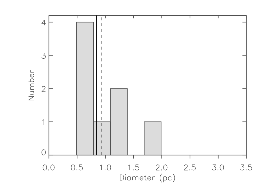
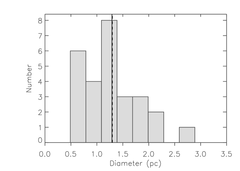
Figure 10: (Left) Histogram of diameters for the eight near IM SFRs. The solid line represents the median size (0.8 pc) while the dashed line represents the average size (0.9 pc). (Right) Histogram of diameters of the 27 IM SFRs that have assigned distances. The solid line represents the median size (1.3 pc) while the dashed line represents the average size (1.3 pc). The bin size is 0.3 pc.

We can attempt to use the available kinematic distances from the CO associations to convert the angular diameters into (near and far) physical diameters, given in Table 3. We attempted to break the near/far distance degeneracy by considering eight objects among the blobs/shells that are highly likely to be located at the near distance. Seven of them are clearly associated with CO features that morphologically resemble local minima and/or dark lanes in the Spitzer 8.0 $\micron$ images. One of them (IRAS 18412-0440) is clearly associated with an infrared dark cloud (IRDC) as described in Simon et al. (2006). These are likely to be associated with molecular clouds at the near distance, seen in silhouette against the more distant diffuse Galactic emission. The eighth near object (IRAS 18180-1342) is on the outskirts of the molecular cloud associated with the Eagle Nebula (M16, NGC 6611). The Eagle Nebula has a photometric distance of $1.8\pm 0.5$ kpc (Bonatto et al., 2006), putting IRAS 18180-1342 at the near distance. Multipanel images of these eight objects are shown as Figures 2 to 9. Using the angular diameters for these eight near objects, we converted angular sizes into physical diameters. The left panel of Figure 10 shows a histogram of the distribution in physical diameter. The diameters range from 0.5 to 1.7 pc with most objects having a diameter less than 1 pc. The median value (solid line) is 0.8 pc and the average value (dashed line) is 0.9 pc. If instead these objects are considered to be at the far distance, the diameters would range from 2.2 to 8.3 with a median value of 3.0 pc and an average value of 3.8 pc. The diameter of $\sim 1$ pc for IM SFRs is consistent with models for PhotoDissociation Regions (PDRs). The Diaz-Miller et al. (1998) models predict an equilibrium PDR diameter of $\sim 1$ pc for an IM star in both a dust-free and a dusty environment. Other PDR models are also consistent with this rough diameter (Kerton, 2002).

Given the small range in physical size among the near distance objects and the consistency with PDR models, we employed a bootstrap “Standard Ruler” method. Using that method, we assigned a more likely distance to objects that cannot be determined to be at the near distance from clouds/dark lanes or association with sources with known distances. We applied the “Standard Ruler” approach to assign objects to the near distance if they have near distance diameters $\geq 0.5$ pc and far distance diameters $>2.0$ pc. These 14 objects were designated with “N” in Table 3. Objects with near distance diameters $<0.5$ pc and far distance diameters $\leq 2.0$ pc were assigned to be at the far distance. These six objects were designated with “F”. Objects at or above tangent point velocities were assigned the tangent point distance and the corresponding diameter. These seven objects were designated with “T”. IRAS 19012+0505-S was assigned to be near, due to its apparent connection to IRAS 19012+0505-N that was assigned the near distance. Fifteen objects remain unassigned. Thirteen of them have both near and far diameters between 0.5 and 2.0 pc, and two objects have near and far diameters that exceed 2.0 pc. These objects were designated “U”. The right panel of Figure 10 shows the distribution of physical diameters for the 27 IM SFRs that have assigned distances in Table 3 (near, far, and tangent). The diameters range from 0.5 to 2.9 pc, with both median (solid line) and average (dashed line) values being 1.3 pc. If we assume that all the unassigned objects are at the near distance, the median diameter drops to 1.0 pc, and the average drops to 1.2 pc. If instead we assume that all the unassigned objects are at the far distance, the median diameter remains at 1.3 pc, and the average increases to 1.4 pc. Regardless of the choice of distances for the remaining unassigned objects, the mean diameter changes by very little.

4 Spectral Energy Distribution

We performed aperture photometry using circular apertures and background annuli, defined by eye, on the Spitzer pipeline mosaics based on the morphology of each object in the 8.0 and 24 $\micron$ images. Typical aperture radii range between $14\arcsec$ and $162\arcsec$ and are listed in Table 4. The irregular shapes and complex backgrounds near most targets, particularly at 8.0 and 24 $\micron$, in addition to bright stars at the shorter bands, do not easily lend themselves to more quantitative approaches that could uniformly be applied to all bandpasses. Nevertheless, the relatively isolated nature of these objects makes it possible to obtain a meaningful measure of their total flux densities using basic aperture photometry. Figure 11 shows the integrated flux density of one object, IRAS 18180-1342, as a function of aperture size, at each of the four IRAC and the MIPS 24 $\micron$ bandpasses. Note that the radial profiles are similar in each bandpass. The 8.0 and 24 $\micron$ flux densities asymptotically approach $\sim 42$ and $\sim 50$ Jy at a radius of $120\arcsec$. The chosen aperture radius of $76\arcsec$ encompasses about half of this total. Typically, the aperture defined by eye encompasses about half of the asymptotic flux density, while an extended envelope accounts for the other half. In some cases emission from a more extended envelope, and possibly other unrelated emission along the line of sight, exceeds half of the asymptotic flux density. In an effort to measure only the flux density from the immediate vicinity of the IM SFRs, we adopted the by-eye apertures and note that these produce flux densities that are typically a factor of two (0.3 dex) lower than the asymptotic flux densities. Table 4 lists the adopted aperture radii in arcsec and resultant flux densities ($F_{\lambda}$) for each object. Aperture corrections were applied as given by Spitzer SSC webpage handbooks. Specifically, the IRAC aperture correction is of the analytical form $a\cdot e^{-b}+c$ where $b$ depends on aperture and $a$ and $c$ are constants that depend on bandpass. For the 24 $\micron$ MIPS bandpass we estimated the aperture correction based on aperture size and it is typically 1.06. Uncertainties are dominated more by systematic effects stemming from aperture definition than statistical fluctuations, so we conservatively estimated relative systematic uncertainties to be 10% in each band, and added that in quadrature with the uncertainty in the flux calibration at each bandpass. We used IRAC flux calibration uncertainties of $2\%$ (Reach et al., 2005) and a MIPS 24 $\micron$ flux calibration uncertainty of $4\%$ (Engelbracht et al., 2007). Saturation was not an issue for these sources, and total uncertainties are typically $\sim 10\%$ for Spitzer photometry. Since MIPS 70 $\micron$ and 160 $\micron$ mosaics were unavailable at the time of this project, we used the flux densities from the IRAS PSC for the 60 and 100 $\micron$ bands ($\sim 15\%$ flux density uncertainties). All flux densities are listed in Table 4. We then plot the final SEDs, from 3.6 to 100 $\micron$, see for example Figure 2, bottom left.

In the vast majority of cases, the flux density in the shorter wavelength IRAC bands is $\sim 1$ Jy and decreases from 3.6 to 4.5 $\micron$. The SED then rises to a few Jy at 5.8 $\micron$ and continues to rise at 8.0 $\micron$. This SED shape is a signature of PAH dominated objects, owing to the lack of PAH lines within the 4.5 $\micron$ band. All SEDs continue to rise through 24 $\micron$, indicating the presence of hot dust. They are still rising in the IRAS 60 and 100 $\micron$ bands, typically reaching $F_{\nu}(100)\approx 200$ Jy. Typically the IRAS PSC $F_{\nu}(12)$ and $F_{\nu}(25)$ are lower than $F_{8.0}$ and $F_{24}$ found using aperture photometry. This effect is expected for extended sources since the IRAS PSC filter surpresses extended emission, thus underestimating the true flux density. This effect is most dramatic at 12 and 25 $\micron$ (Fich & Terebey, 1996).

4.1 Infrared Luminosities

From the SEDs and distance estimates, the infrared luminosity ($L_{\mathrm{IR}}$) can be estimated. We estimated the flux by integrating under the curve. For the contribution from the IRAS PSC flux densities, the method of Emerson (1988) is used to obtain the contribution to the fluxes. We obtain the luminosities (near and far) by multiplying the fluxes by $4\pi d^{2}$, where $d$ is the distance (near and far). These infrared luminosities are listed in Table 4. These tabulated luminosities are lower limits since they do not consider contributions from wavelengths longer than 135 $\micron$ (the edge of the IRAS 100 $\micron$ bandpass). Comparison of IRAS-derived luminosities with SEDs from the Diffuse Infrared Background Experiment (DIRBE) and the Balloon-borne Large Aperture Submillimeter Telescope (BLAST) suggest that we are missing $\sim 10\%$ of the total luminosity (Kerton, 2000; Chapin et al., 2008)

The distribution of $L_{\mathrm{IR}}$ for the near eight objects is shown as a histogram in Figure 12 (left). The luminosities range from $7\times 10^{2}$ to $3.7\times 10^{4}$ L_☉. Most are less than $10^{4}$ solar luminosities, which is reflected in a median value of $4.9\times 10^{3}$ L_☉ (solid line) and an average value of $8.4\times 10^{3}$ L_☉ (dashed line). If instead these objects were considered to be at the far distance, the luminosities would range from $1.4\times 10^{4}$ to $3.3\times 10^{5}$ L_☉, with a median value of $7.0\times 10^{4}$ L_☉ and an average value of $1.2\times 10^{5}$ L_☉.

The right panel of Figure 12 shows a histogram of the distribution of $L_{\mathrm{IR}}$ for the 27 objects that have assigned distances. The luminosities range from $7\times 10^{2}$ to $1.1\times 10^{5}$ L_☉. The median value is $9.2\times 10^{3}$ L_☉ (solid line) and the average value is $1.5\times 10^{4}$ L_☉ (dashed line). We find that this luminosity range is consistent with recent models of YSO SEDs (Robitaille et al., 2006). Figure 13 shows the model YSO luminosities of a range of objects that have optically thick disks (Stage II) as a function of stellar mass. Evidently, $10^{3}$ to $10^{4}$ L_☉ corresponds roughly to $\sim 4-10$ M_☉ YSOs, i.e., intermediate-mass. In Section 6.1, we compare this range in luminosity to luminosities of UCH II regions, showing that IM SFRs and UCH II regions are quite distinct sets.

5 Molecular Material and Masses

In this section, we investigate the molecular material that is spatially associated with the IM SFRs, using the corresponding zeroth-moment maps. Usually, the location of the maximum value in the zeroth-moment map (i.e., the peak integrated intensity) for the local CO “clump” lies outside of the mid-IR blob/shell seen in Spitzer mosaics. Table 5 lists the IRAS name for sources having a velocity association from Table 3, the peak integrated intensity ($I_{\mathrm{peak}}$), the corresponding peak H₂ column density ($N(\mathrm{H_{2}})_{\mathrm{peak}}$) and peak mass column density ($N(M)_{\mathrm{peak}}$), the solid angle ($\Omega$) occupied by the CO clump (used to calculate the mass), the flag from Table 3 indicating distance assumption, the near and far distance clump masses ($M_{\mathrm{LTE}}$), the parent GRS Molecular Cloud (GRSMC), associated GRSMC-clump, the mass of the GRSMC ($M_{\mathrm{Cloud}}$), and a note on the distance determination of the GRSMC.

5.1 Column densities and masses from CO/H₂

To estimate column densities and molecular masses from GRS CO observations, we assumed an optically thin, LTE (CO is almost always close to LTE, see Rohlfs & Wilson, 2004) situation for the ¹³CO $J=1\rightarrow 0$ rotational line. Furthermore, we assumed the excitation temperature is approximately equal the main beam temperature; typically $\sim 10$ K for dense cold molecular material. The derived ¹³CO column densities are only weakly sensitive to the exact choice of the excitation temperature, changing it to 20 K increases the derived mass by 40% (Simon et al., 2001). Under these assumptions, the expression for the column density of ¹³CO is (Rohlfs & Wilson, 2004, eq. 14.40),

$${}N({{}^{13}\mathrm{CO}})=7.3\times 10^{14}\int T_{\mathrm{MB}}\mathrm{d}V~{}\mathrm{cm}^{-2}$$ (1)

Using conversion factors from Simon et al. (2001) and references therein (R(¹²CO/¹³CO$)=45$ and R(¹²CO/H${}_{2})=8\times 10^{-5}$) we calculated the peak H₂ column density ($N(\mathrm{H_{2}})_{\mathrm{peak}}$) in cm^-2. We got the peak mass column density by multiplying $N(\mathrm{H_{2}})_{\mathrm{peak}}$ with the H₂ molecular mass and a factor of 1.36 to account for elements heavier than hydrogen (Simon et al., 2001). Summing over the area of the CO clump, we obtained the (near and far distance) clump mass, given in Table 5.

The uncertainty in the mass calculation is dominated by the background determination, and is estimated to be $\sim 10\%$. More importantly, subthermal excitation of higher rotational levels may result in an overestimate of the column density. This overestimate would be of the same order as the underestimate due to moderate opacity effects. This, taken together with the above assumptions, make column densities and derived masses lower limits, that are estimated to be accurate within a factor of a few (Simon et al., 2001).

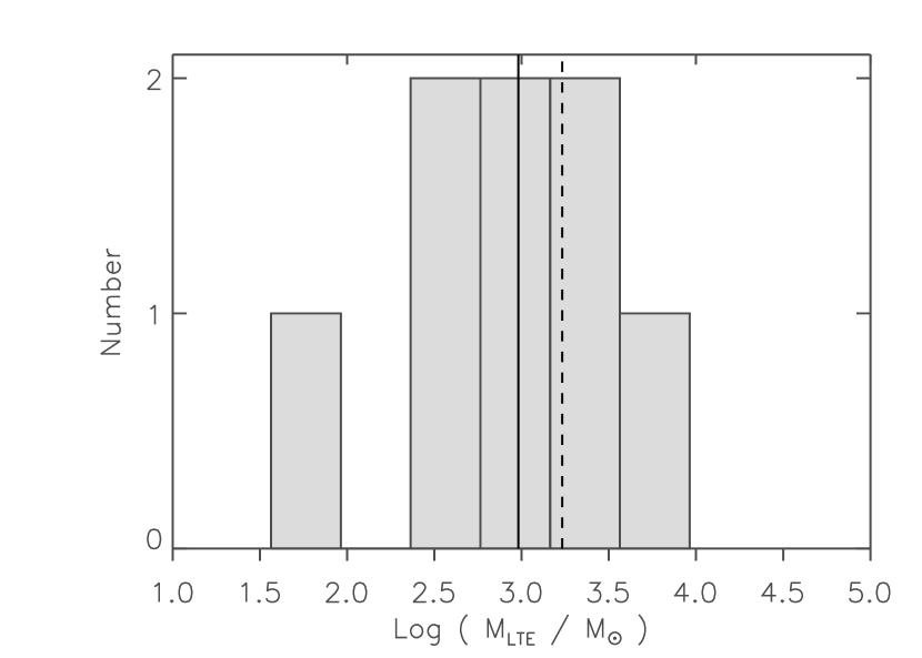
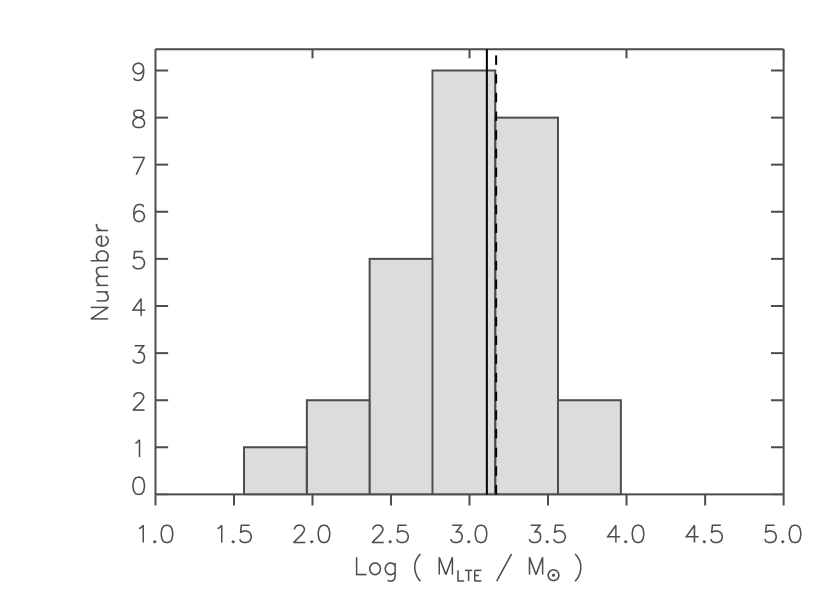
Figure 14: (Left) Histogram of $\log(M_{\mathrm{LTE}}/M_{\sun})$ for the local molecular material associated with the eight near IM SFRs. The solid line represents $\log(\mathrm{median})=3.0$ while the dashed line represents $\log(\mathrm{average})=3.2$. (Right) Histogram of $\log(M_{\mathrm{LTE}}/M_{\sun})$ for the local molecular material associated with the 27 IM SFRs that have assigned distances. The solid line represents $\log(\mathrm{median})=3.1$ while the dashed line represents $\log(\mathrm{average})=3.2$. The bin size is 0.4 dex.

The median and average peak mass column density obtained this way is 0.03 g cm^-2 with a maximum of 0.08 g cm^-2. The mass of the local molecular material associated with the eight near sources, $M_{\mathrm{LTE}}$, range from 40 M_☉ to 2800 M_☉, and Figure 14 (left) shows a histogram of this distribution. The median of the masses is 900 M_☉ (solid line) and the average is 1700 M_☉ (dashed line). If instead these objects were considered to be at the far distance, the masses would range from $1.8\times 10^{3}$ M_☉ to $5.6\times 10^{5}$ M_☉, with a median value of $1.4\times 10^{4}$ M_☉ and an average value of $1.9\times 10^{4}$ M_☉. The right panel of Figure 14 shows a histogram of the distribution of $M_{\mathrm{LTE}}$ for the molecular material associated with the 27 objects that have assigned distances. The masses range from 40 M_☉ to 6100 M_☉, with a median of 1300 M_☉ (solid line) and an average of 1500 M_☉ (dashed line).

5.2 Column densities and masses from BGPS

Out of the 50 objects, the CO material is spatially associated with a millimeter-wave continuum source from the BGPS catalog (Rosolowsky et al., 2010) in 28 objects, 10 objects have no BGPS source associated, and 12 objects are not covered by the BGPS. Typically for an association, the BGPS continuum source is located on or very near the location of $I_{\mathrm{peak}}$. For some objects there are several BGPS sources within the CO feature, but Table 6 only lists the source closest to $I_{\mathrm{peak}}$. The peak brightness within the BGPS source, $F_{\mathrm{peak}}$, is related to the peak column density, $N(\mathrm{H_{2}})_{\mathrm{peak}}$, through the conversion factor of $N(\mathrm{H_{2}})/F=6.77\times 10^{19}$ cm^-2 (mJy beam${}^{-1})^{-1}$ (Table A.1 in Kauffmann et al., 2008). From the the peak H₂ column density traced by millimeter continuum emission we obtain the peak mass column density as in Section 5.1. We note that column densities derived in this manner are lower limits for unresolved sources in the BGPS. The peak mass column densities traced by the BGPS are typically $\sim 0.1$ g cm^-2, with a minimum of 0.05 g cm^-2 and a maximum of 0.5 g cm^-2. These peak mass column densities are higher than the corresponding peak mass column densities determined using the GRS. This is likely an effect of ¹³CO becoming optically thick in the denser regions.

Out of the 28 BGPS sources, 22 have velocities from CO associations. 15 of them have distance determinations while seven do not. Using the integrated flux density $S$ from the BGPS catalog together with our distance estimates, the source masses can be estimated using (Rosolowsky et al., 2010, eq. 10),

$${}M=13.1\mathrm{M}_{\sun}\left(\frac{d}{1~{}\mathrm{kpc}}\right)^{2}\left(\frac{S}{1~{}\mathrm{Jy}}\right)\left[\frac{\exp(13.0~{}\mathrm{K}/T)-1}{\exp(13.0/20)-1}\right]$$ (2)

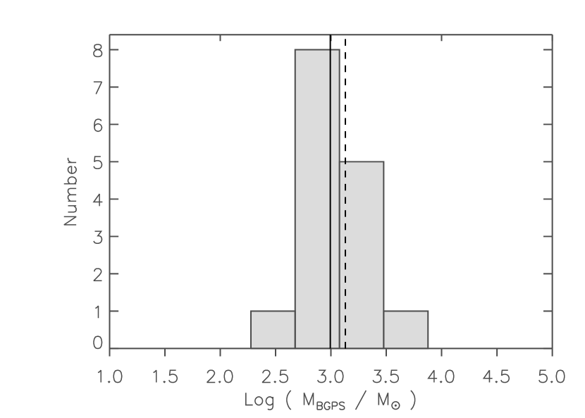
Figure 15: Histogram of $\log(M_{\mathrm{BGPS}}/M_{\sun})$ for the 15 objects with assigned distances that are associated with BGPS sources. The solid line represents $\log(\mathrm{median})=3.0$ while the dashed line represents $\log(\mathrm{average})=3.1$. The object with the highest $M_{\mathrm{BGPS}}$ in the figure is IRAS 18502-0018, an object dominated by an H II region (see Section 7). The bin size is 0.4 dex.

where we use $T=10$ K like before. The results are given in Table 6. Figure 15 shows a histogram of the distribution of $M_{\mathrm{BGPS}}$ for the 15 objects with distance determinations. The masses range from 200 M_☉ to 6700 M_☉, with a median of 1000 M_☉ (solid line) and an average of 1400 M_☉ (dashed line). This result largely agrees with CO-based mass estimates.

5.3 Molecular Clouds

To investigate the possibility that IM SFRs are only found in low mass molecular clouds, we use the catalog of GRS molecular clouds (GRSMCs; Rathborne et al., 2009) to identify the large scale molecular clouds containing the IM SFRs. The identification was made by comparing the locations and velocities of so called “clumps” in Rathborne et al. (2009) to our identifications of molecular material. An identification was made if the clump has a tabulated velocity within $\sim 1$ km s^-1 of the velocity listed in Table 3 and has a position centered on or very near the location of $I_{\mathrm{peak}}$. In 28 out of 42 cases we were able to associate a clump with a particular molecular cloud (see Table 5).

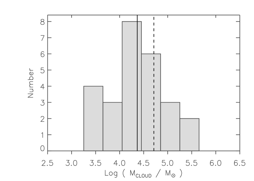
Figure 16: Histogram of $\log(M_{\mathrm{Cloud}}/M_{\sun})$ for the 26 GRSMCs associated with the IM SFRs. The four GRSMCs listed as (!) in Table 5 have been scaled to the near distance using $d_{near}$ from Table 3. The solid line represents $\log(\mathrm{median})=4.4$ while the dashed line represents $\log(\mathrm{average})=4.7$. The bin size is 0.4 dex.

Roman-Duval et al. (2009) lists distances to 26 of the 28 GRSMCs we found to be associated with IM SFRs. We note that none of these GRSMCs have strong 21 cm continuum sources associated with them, therefore the kinematic distance ambiguity was resolved by the presence or absence of H I self-absorption (HISA). Only four of the 26 GRSMC distance determinations disagree with our IM SFR standard ruler method determinations, they are marked as (!) in Table 5. We use the ¹³CO luminosity ($L(^{13}$CO)) of the cloud from Roman-Duval et al. (2009) and the same conversion factors used in Section 5.1 to compute the cloud mass. The results of the calculations are listed in Table 5. Figure 16 shows a histogram of the 26 GRSMC masses where the four GRSMCs listed as (!) in Table 5 have been recalculated using the near distance $d_{near}$ from Table 3. The GRSMC masses range from 1800 M_☉ to $2.3\times 10^{5}$ M_☉, with a median of $2.3\times 10^{4}$ M_☉ (solid line) and an average of $5.1\times 10^{4}$ M_☉ (dashed line). These fall toward the lower end of the range in mass expected of Giant Molecular Clouds (GMCs; $10^{4}-10^{6}$ M_☉).

6 Comparison to UCH II regions

UCH II regions are manifestations of newly formed massive stars that are still embedded in their natal molecular clouds. They are small ($<0.1$ pc), dense ($>10^{4}$ cm^-3), bright photoionized nebulae. At IRAS 100 $\micron$ they are among the brightest objects in the Galaxy because of the warm dust envelope converting the entire stellar luminosity into FIR radiation. We compare these relatively well-studied objects to our IM SFRs and show that UCH II regions are quite distinct from IM SFRs in luminosity, in column density, and in the mass of associated material traced with millimeter-wave continuum emission.

6.1 UCH II region luminosities

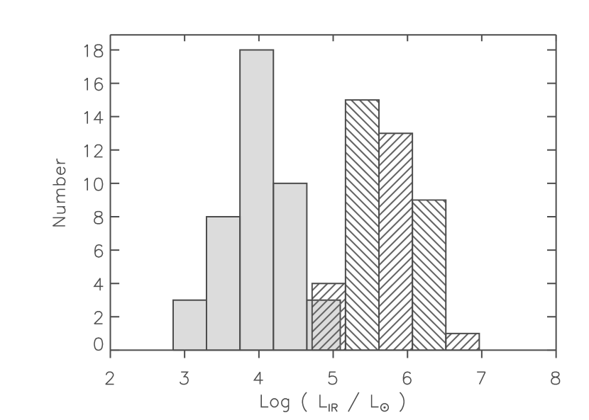
Figure 17: Histogram of $\log(L_{\mathrm{IR}}/L_{\sun})$ for 42 IM SFR luminosities (shaded, with unassigned objects assumed to be at the far distance) and for 42 UCH II region luminosities (barred) from Wood & Churchwell (1989a). The luminosity distribution is bi-modal, with UCH II regions and IM SFRs forming two distinct populations separated by roughly an order of magnitude. The IM SFR overlap consists of unassigned objects and IRAS 18502-0018, an object dominated by an H II region (see Section 7). The bin size is 0.45 dex.

Figure 17 shows a histogram of the infrared luminosities ($L_{\mathrm{IR}}$) of the IM SFRs (shaded), with all the objects labeled Unassigned (“U” in Table 3) assumed to be at the far distance (as a most extreme case scenario). The barred histogram shows $L_{\mathrm{IR}}$ for 42 of the UCH II regions in Table 18 of Wood & Churchwell (1989a). In both cases contributions to $L_{\mathrm{IR}}$ from wavelengths longer than the edge of the IRAS 100 $\micron$ bandpass were not considered, and so in both cases $L_{\mathrm{IR}}$ are lower limits to the bolometric luminosities. The luminosity distribution is bi-modal, with UCH II regions and IM SFRs forming two distinct populations separated by roughly an order of magnitude. In fact, the overlapping region at the higher end of the IM SFR luminosity distribution (shaded) consists of objects with unassigned distances (which were all assumed at the far distance for the figure). If they instead were assumed to be at near distance only one object would overlap with the lower end of the UCH II region distribution, and that object turns out to be dominated by an H II region (IRAS 18502-0018, see Section 7). Comparing the median (or average) shows that UCH II regions are typically 40–80 times more luminous than IM SFRs.

6.2 UCH II regions in the BGPS

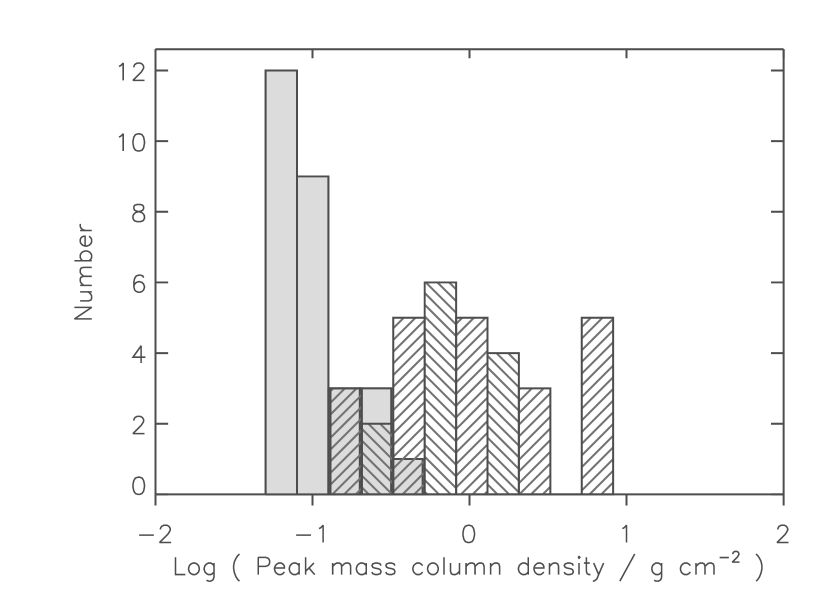
Figure 18: Histogram of the peak mass column density, $\log(N(M)_{\mathrm{peak}}/\mathrm{g~{}cm}^{-2})$ for the material associated with 28 IM SFRs, traced by millimeter-wave continuum (shaded) and for the material associated with 33 UCH II regions (barred). The mass column density distribution is roughly bi-modal, with UCH II regions and IM SFRs forming two populations separated by roughly an order of magnitude. The bin size is 0.2 dex.

We examined the positions of UCH II regions with adopted distances (Table 4 in Wood & Churchwell, 1989a) by eye for association with a millimeter-wave continuum source from the BGPS catalog (Rosolowsky et al., 2010). For 33 UCH II regions, an associated BGPS source is found. Using the same technique used for IM SFRs in Section 5.2 we calculate peak mass column densities toward these UCH II regions. Figure 18 shows peak mass column densities for IM SFRs (shaded) and UCH II regions (barred). The peak mass column density distribution is roughly bi-modal, with UCH II regions and IM SFRs forming two populations separated by roughly an order of magnitude. Comparing the median (or average) shows that peak mass column densities for the material associated with UCH II regions are typically $\sim 10$ times greater than for IM SFRs.

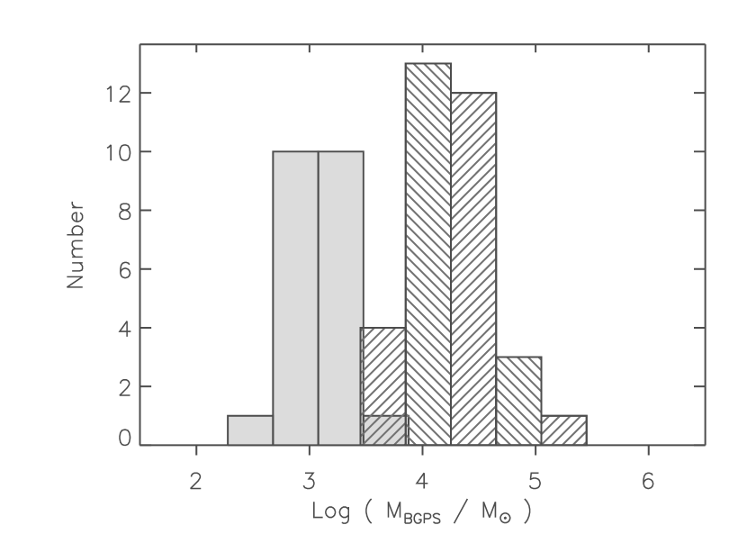
Figure 19: Histogram of $\log(M_{\mathrm{BGPS}}/M_{\sun})$ for the material associated with 22 IM SFRs, traced by millimeter-wave continuum (shaded, with unassigned objects assumed to be at the far distance) and for the material associated with 33 UCH II regions (barred). The mass distribution is bi-modal, with UCH II regions and IM SFRs forming two distinct populations separated by roughly an order of magnitude. The IM SFR overlap consists of IRAS 18502-0018, an object dominated by an H II region (see Section 7). The bin size is 0.4 dex.

We use equation 2 with the same assumptions as in Section 5.2 together with the adopted distances from Table 4 in Wood & Churchwell (1989a) to compute the masses of the cold, dense material associated with the UCH II regions. The masses of the material associated with UCH II regions is shown as the barred histogram in Figure 19 while the shaded histogram is the mass of the material closely associated with the IM SFRs (from Table 6, with unassigned objects being assumed to be at the far distance). As with the distributions of luminosities and peak mass column densities, the masses of the closely associated material form a bi-modal distribution, with UCH II regions and IM SFRs forming two populations separated by roughly an order of magnitude. The one overlapping shaded object is again IRAS 18502-0018. Comparing the median (or average) of the two populations shows material associated with UCH II regions is typically $\sim 20$ times more massive than the material associated with IM SFRs.

7 Discussion

Radio continuum images from the NRAO/VLA Sky Survey (NVSS; Condon et al., 1998) at 1.42 GHz show that all but one of the investigated blobs/shells lack 1.42 GHz continuum emission from H II. NVSS has a $45\arcsec$ FWHM resolution and rms brightness uncertainties of about $\sim 0.45$ mJy beam${}^{-1}\approx 0.14$ K (Stokes I). The completeness limit is about 2.5 mJy. Radio continuum measurements of H II regions can provide a lower limit on the total number of ionizing photons ($N_{L}$),

$${}N_{L}\geq 7.5\times 10^{43}S_{\nu}d^{2}\nu^{0.1}T_{e}^{-0.45}~{}\textrm{s}^{-1}\\$$ (3)

where $\nu$ is the frequency in GHz, $S_{\nu}$ is the flux density measured at frequency $\nu$ in mJy, $d$ is the distance to the source in kpc, and $T_{e}$ is the electron temperature in units of $10^{4}$ K (Rudolph et al., 1996). This assumes an optically thin, spherical, constant-density H II region. Given the adopted distances in Table 3, a $3\sigma$ NVSS detection would correspond to about $\log(N_{L})\sim 45$ (with a maximum of 46.1). For comparison, a B0.5 V star powered H II region has $\log(N_{L})=47.77$ (Schaerer & de Koter, 1997) and would easily be detected at a $3\sigma$ level in NVSS if $d\lesssim 75$ kpc.

Highly embedded massive stars can potentially be radio quiet due to the absorption of ultra-violet photons by surrounding dust. We think it is very unlikely that we are probing massive stars at such a very early stage because our sample’s range in luminosity, total molecular mass and mass column density are all much lower than those associated with regions of known massive star formation. We conclude that the lack of radio continuum emission in these sources is consistent with our interpretation of them as IM SFRs. To confirm the IM nature of these sources, direct IR spectroscopical observations of the YSO content in these sources are being planned.

The only apparent exception, IRAS 18502-0018, actually consists of a $0.4\arcmin$ blob located on the edge of a dusty $2.5\arcmin$ diameter H II region. Applying the standard ruler technique to the $0.4\arcmin$ blob results in a distance of 11.1 kpc, which agrees with the distance found for the associated GRSMC (Roman-Duval et al., 2009). The 1.42 GHz continuum emission associated with the H II region has a flux density of $S_{\nu}=126.7\pm 5.1$ mJy in the NVSS catalog. This corresponds to $\log(N_{L})=48.1$ or a single B0 V star (Schaerer & de Koter, 1997). We interpret this region as a possible IM SFR sitting on the edge of a dusty shell surrounding a small H II region.

We found that the large-scale molecular environment associated with IM SFRs is similar to that associated with high-mass star formation; IM SFRs are found in molecular clumps of $\sim 10^{3}$ M_☉ sitting within Giant Molecular Clouds (GMCs) with a range of masses between $10^{4}-10^{5}$ M_☉. The implication of this result is that massive star formation, while possible in GMCs in this mass range, is not inevitable. IM SFRs are also associated with lower mass $\sim 10^{2}$ M_☉ clumps, much lower than those associated with high mass star formation (Zinnecker & Yorke, 2007). In contrast, no IM SFRs are found in GMCs with masses $\gtrsim 10^{6}$ M_☉, suggesting that for the most massive GMCs, high-mass stars will always form.

The left hand panel of Figure 20 shows a strong correlation between luminosity and associated clump mass for both IM SFRs and UCH II regions. The data are fit by $L\propto M^{1.12\pm 0.08}$ which agrees with the mass-luminosity relationship found by Chini et al. (1987) that was derived using only a sample of compact H II regions. This relationship clearly holds over three orders of magnitude, a result only hinted at in Chini et al. (1987).

In the right panel of Figure 20 we plot luminosity versus peak mass column density for our sample of IM SFRs and UCH II regions. Krumholz & McKee (2008) provide a theoretical expectation that mass column densities $\gtrsim 1$ g cm^-2 are needed for massive star formation. We observe the maximum mass column density for IM SFRs is 0.5 g cm^-2 and both the median and the average are $\sim 0.1$ g cm^-2, all well below the proposed threshold. A simple interpretation of the data shown in the right panel of Figure 20 is that if the mass column density is above 1 g cm^-2, only massive stars will form, below 1 g cm^-2 you can form intermediate through massive stars, and at or below 0.1 g cm^-2, no massive stars will form.

As this paper went to press, we became aware of the methanol maser survey of Pandian & Goldsmith (2007) who report methanol masers near two of the candidate IM SFRs studied here: 19012+0505-N (as 38.92-0.36) and 19049+0712 (as 41.23-0.20). These two IM SFRs, along with 18224-1228, were also detected in previous methanol maser surveys (Szymczak et al., 2000; Pestalozzi et al., 2005). Methanol masers are believed to occur during the early phases of massive star formation. Association with some of the IM SFRs suggests either that some of our sample objects are more massive (and possibly more distant) than inferred here, or that intermediate-mass star-forming regions are also capable of producing maser activity. Interestingly, these three sources having methanol maser associations (18224-1228, 19012+0505N, and 19049+0712) are flagged in Table 5 as having previous distance determinations (based on the absence of HISA; Roman-Duval et al., 2009; Pandian et al., 2009) that would place them at the far kinematic distance, resulting in larger luminosities and molecular masses that would make them similar to some of the least luminous UCH II regions in our comparison sample.

8 Conclusions

We have identified a sample of 50 IM SFRs in the inner Galaxy. The IM SFRs share some basic properties. They have typical luminosities of $\sim 10^{4}$ L_☉ and the PDRs that demarcate the IM SFRs have typical diameters of $\sim 1$ pc. All but one lack radio continuum emission and some show small stellar clusters visible in the NIR. These properties are consistent with these objects being regions containing stars in the $2-8$ M_☉ range with their associated clusters of low-mass stars. The most massive stars in these regions are likely to be precursors to Herbig AeBe stars.

IM SFRs do show some similarities with high-mass star-forming regions. On parsec-scales IM SFRs are typically associated with molecular clumps of mass $\sim 10^{3}$ M_☉ and on larger scales they are found within GMCs with masses between $10^{4}-10^{5}$ M_☉. We conclude that massive star formation in GMCs in that mass range is not inevitable.

IM SFRs are also distinct from regions of more massive star formation, forming in clumps with masses as low as $\sim 10^{2}$ M_☉ and not being found in the most massive GMCs ($\gtrsim 10^{6}$ M_☉). IM SFRs typically have an order of magnitude less luminosity than UCH II regions.

Our sample of IM SFRs, combined with UCH II region data, shows that a strong correlation between luminosity and associated molecular mass in star-forming regions applies over three orders of magnitude encompassing both IM SFRs and UCH II regions.

The molecular material associated with IM SFRs typically have an order of magnitude smaller peak mass column density and clump mass compared to UCH II regions. The lack of IM SFRs found with associated peak mass column densities $>0.5$ g cm^-2 supports the idea that there is a threshold in mass column density above which only massive star formation occurs.

Table 1: Number of potential sources.

Region	Number of sources
All sky	984
Galactic plane	360
($|b|<1\arcdeg$)
GLIMPSE I	178
$(10\arcdeg<|\ell|<65\arcdeg$, $|b|<1\arcdeg)$
GRS	70
$(18\arcdeg<\ell<55\fdg 7$, $|b|<1\arcdeg)$

Note. — Number of IRAS point sources for various regions using the color criteria from Kerton (2002): $-0.18<\log(F_{\nu}(25)/F_{\nu}(12))<0.40$, $0.96<\log(F_{\nu}(60)/F_{\nu}(25))<1.56$ and $0.29<\log(F_{\nu}(100)/F_{\nu}(60))<0.69$.

Table 2: Filamentary and star-like objects.

IRAS name	$\ell$	$b$	Class
	($\arcdeg$)	($\arcdeg$)
18163-1603	15.03450	$-0.35301$	F
18169-1338	17.23340	$0.68040$	F
18227-1218	19.07937	$0.06120$	F
18257-1226	19.30243	$-0.65138$	S
18279-1039	21.12765	$-0.28842$	F
18317-0926	22.63746	$-0.54983$	S
18328-0900	23.14221	$-0.58687$	S
18318-0741	24.20073	$0.25168$	S
18416-0518	27.43590	$-0.81472$	S
18465-0018	32.44363	$0.39727$	S
18559+0308	36.58437	$-0.09614$	S
18571+0326	36.99180	$-0.22897$	F
18550+0358	37.22322	$0.47883$	F
18588+0350	37.54749	$-0.40816$	S
19040+0616	40.30611	$-0.43082$	F
19079+0919	43.45117	$0.11756$	F
19137+1013	44.92225	$-0.71903$	F
19150+1116	45.98566	$-0.50465$	S
19152+1209	46.80001	$-0.12841$	F
19273+1637	52.11558	$-0.57587$	S
19300+1852	54.38650	$-0.03721$	F

Note. — Filamentary and star-like objects. Listed are the IRAS PSC names, the Galactic longitudes ($\ell$), Galactic latitudes ($b$), and the classifications. Filamentary objects are denoted with a “F”, and star-like objects with a “S”.

Table 3: IM SFRs - Properties of blobs and shells.

IRAS name	$\ell$	$b$	$\theta$	$V_{\mathrm{LSR}}$	$\Delta V$	$d_{\mathrm{near}}$	$d_{\mathrm{far}}$	Adopted	Flag	Diameter	$L_{\mathrm{IR}}$	$M_{\mathrm{LTE}}$
	($\arcdeg$)	($\arcdeg$)	($\arcmin$)	(km s-1)	(km s-1)	(kpc)	(kpc)	(kpc)		(pc)	($10^{3}$ L☉)	(M☉)
18131-1606	14.63111	$0.30075$	1.0	$26.1$	8.2	2.9	13.6	2.9	N	0.8	10.7	500
18180-1342	17.31025	$0.40066$	2.0	$19.7$	3.7	2.0	14.2	2.0	N	1.2	4.9	40
18241-1320	18.32426	$-0.73709$	0.6	$43.3$	4.4	3.7	12.5	3.7	N	0.6	1.2	800
18224-1228	18.88269	$0.05205$	1.5	$49.9$	9.3	4.0	12.1	4.0	N	1.7	36.5	6100
18253-1210	19.50327	$-0.44381$	1.0	$63.1$	5.0	4.6	11.4	4.6	N	1.3	6.0	2800
18322-0956	22.25764	$-0.87999$	0.6	$41.0$	2.6	3.2	12.5	3.2	N	0.6	4.6	200
18308-0741	24.09699	$0.45326$	1.8	$94.7$	8.2	5.9	9.6	$\cdots$	U	3.1/5.0	27.7/73.3	4300/11500
18370-0607	26.19714	$-0.18673$	0.6	$108.3$	4.5	7.6	7.6	7.6	T	1.3	15.0	1700
18367-0529	26.71852	$0.17412$	0.5	$\cdots$	$\cdots$	$\cdots$	$\cdots$	$\cdots$	A	$\cdots$	$\cdots$	$\cdots$
18362-0517	26.83021	$0.38216$	2.2	$\cdots$	$\cdots$	$\cdots$	$\cdots$	$\cdots$	A	$\cdots$	$\cdots$	$\cdots$
18412-0440	27.96505	$-0.44254$	0.8	$45.6$	7.8	3.1	11.9	3.1	N	0.7	2.4	2300
18411-0312	29.24142	$0.25972$	0.5	$\cdots$	$\cdots$	$\cdots$	$\cdots$	$\cdots$	A	$\cdots$	$\cdots$	$\cdots$
18433-0327	29.28703	$-0.33671$	0.5	$\cdots$	$\cdots$	$\cdots$	$\cdots$	$\cdots$	A	$\cdots$	$\cdots$	$\cdots$
18441-0118	31.27801	$0.48597$	1.5	$89.2$	14.4	5.8	8.8	$\cdots$	U	2.5/3.8	5.7/13.2	2100/4900
18463-0052	31.91297	$0.19629$	1.0	$107.9$	7.3	7.2	7.2	7.2	T	2.1	29.0	1600
18502-0018	32.86081	$-0.41053$	0.4	$48.0$	9.2	3.2	11.1	11.1	F	1.3	110.3	2600
18504+0025	33.53779	$-0.12907$	0.5	$\cdots$	$\cdots$	$\cdots$	$\cdots$	$\cdots$	A	$\cdots$	$\cdots$	$\cdots$
18537+0145	35.09790	$-0.24120$	0.5	$51.6$	7.6	3.4	10.6	$\cdots$	U	0.5/1.5	4.4/42.9	100/900
18527+0203	35.26396	$0.12033$	1.0	$\cdots$	$\cdots$	$\cdots$	$\cdots$	$\cdots$	A	$\cdots$	$\cdots$	$\cdots$
18564+0145	35.41394	$-0.84999$	0.7	$36.7$	6.2	2.4	11.4	2.4	N	0.5	0.7	1000
19014+0451	38.75274	$-0.52447$	0.5	$66.2$	7.8	4.5	8.7	$\cdots$	U	0.7/1.3	4.9/18.5	200/800
19012+0505-N	38.92659	$-0.37007$	1.8	$39.8$	6.7	2.6	10.6	2.6	N	1.4	10.7	700
19012+0505-S	38.92659	$-0.37007$	3.0	$41.3$	6.7	2.7	10.5	2.7	N	2.4	9.0	1400
19023+0545	39.64763	$-0.29262$	0.6	$25.8$	4.8	1.8	11.3	11.3	F	2.0	26.6	200
19023+0601	39.87238	$-0.17333$	1.3	$57.3$	12.4	3.8	9.2	3.8	N	1.4	8.0	200
19027+0656	40.74324	$0.15801$	0.5	$16.9$	8.8	1.3	11.6	11.6	F	1.7	17.1	3100
19060+0657	41.14428	$-0.56201$	2.2	$\cdots$	$\cdots$	$\cdots$	$\cdots$	$\cdots$	A	$\cdots$	$\cdots$	$\cdots$
19072+0649	41.14722	$-0.88475$	0.5	$66.5$	6.0	4.9	7.9	$\cdots$	U	0.7/1.1	2.1/5.5	700/1700
19049+0712	41.22959	$-0.19367$	1.0	$59.4$	6.3	4.1	8.7	4.1	N	1.2	10.2	400
19062+0758	42.05222	$-0.11977$	1.2	$70.3$	6.9	5.6	7.1	5.6	N	2.0	3.8	1600
19105+0852	43.35147	$-0.66408$	0.6	$58.0$	6.3	4.2	8.2	$\cdots$	U	0.7/1.4	3.3/12.5	500/1800
19056+0947	43.59957	$0.85377$	0.8	$\cdots$	$\cdots$	$\cdots$	$\cdots$	$\cdots$	No CO	$\cdots$	$\cdots$	$\cdots$
19139+1045	45.40416	$-0.51347$	1.1	$60.9$	11.1	4.9	7.0	4.9	N	1.6	9.2	300
19138+1055	45.53808	$-0.39856$	0.7	$57.7$	13.3	4.5	7.4	$\cdots$	U	0.9/1.5	3.0/8.0	1000/2600
19157+1319	47.87449	$0.31098$	0.4	$63.5$	5.5	5.7	5.7	5.7	T	0.7	4.5	1400
19207+1329	48.60178	$-0.66833$	0.5	$52.6$	11.8	4.4	6.9	$\cdots$	U	0.6/1.0	2.9/7.2	500/1200
19207+1348	48.87743	$-0.51817$	0.6	$57.3$	5.0	5.6	5.6	5.6	T	1.0	33.4	4300
19156+1441	49.07458	$0.98102$	0.4	$53.1$	4.7	4.5	6.6	$\cdots$	U	0.5/0.8	0.8/1.7	300/600
19193+1443	49.53260	$0.20918$	0.5	$63.1$	5.5	5.5	5.5	5.5	T	0.8	4.2	600
19233+1413	49.54016	$-0.88136$	0.5	$43.3$	8.0	3.3	7.7	$\cdots$	U	0.5/1.1	2.9/16.1	600/3200
19205+1447	49.72280	$-0.01595$	0.6	$48.2$	10.4	3.9	7.1	$\cdots$	U	0.7/1.2	13.4/44.5	2000/6700
19221+1456	50.03463	$-0.28204$	1.8	$61.8$	10.4	5.5	5.5	5.5	T	2.9	16.3	1300
19214+1556	50.84320	$0.33493$	0.7	$40.5$	8.4	3.2	7.6	$\cdots$	U	0.7/1.5	2.7/15.3	1000/5400
19255+1531	50.93431	$-0.72378$	0.6	$38.6$	5.1	3.0	7.7	$\cdots$	U	0.5/1.3	2.2/14.3	300/1800
19256+1705	52.33394	$0.00598$	0.5	$12.0$	5.4	1.1	9.3	9.3	F	1.4	9.7	600
19248+1730	52.60285	$0.37402$	0.7	$41.2$	10.1	3.5	6.8	$\cdots$	U	0.7/1.4	1.9/7.0	100/500
19247+1829	53.44999	$0.87096$	0.4	$-2.6$	4.4	0.3	9.9	9.9	F	1.2	6.9	1300
19260+1821	53.48407	$0.52532$	0.4	$49.9$	6.7	5.1	5.1	5.1	T	0.6	2.1	2000
19266+1926	54.51342	$0.92616$	0.6	$32.4$	7.1	2.7	7.1	$\cdots$	U	0.5/1.2	2.5/17.5	400/2500
19330+1956	55.66724	$-0.13004$	0.5	$31.6$	5.6	2.8	6.9	6.9	F	1.0	10.2	900

Note. — Properties of the objects labeled as blobs or shells. $\theta$ is the angular diameter. $V_{\mathrm{LSR}}$ is the associated CO velocity from the GRS, and $\Delta V$ is the width of the associated CO feature. $d_{\mathrm{near}}$ and $d_{\mathrm{far}}$ are the near and far distances. Adopted indicates the value for the distance used in subsequent analysis. The flags are: “N” for near, “F” for far, “T” for tangent point, “U” for unassigned, and “A” for ambiguous CO association. The diameter is calculated using the adopted distance. $L_{\mathrm{IR}}$ is taken from Table 4, and $M_{\mathrm{LTE}}$ from Table 5.

Table 4: IM SFRs - Photometry and luminosity.

IRAS name	Aperture	F3.6	$\sigma_{3.6}$	F4.5	$\sigma_{4.5}$	F5.8	$\sigma_{5.8}$	F8.0	$\sigma_{8.0}$	F24	$\sigma_{24}$	F${}_{\nu}(60)$	$F_{\nu}(100)$	Flag	$L_{\mathrm{near}}$	$L_{\mathrm{far}}$
	($\arcsec$)	(Jy)	(Jy)	(Jy)	(Jy)	(Jy)	(Jy)	(Jy)	(Jy)	(Jy)	(Jy)	(Jy)	(Jy)		($10^{3}$ L☉)	($10^{3}$ L☉)
18131-1606	54	2.28	0.23	1.47	0.15	6.60	0.68	14.74	1.51	42.39	5.67	305.0	799.3	N	10.7	234.3
18180-1342	76	3.78	0.54	3.05	0.31	11.68	1.20	29.40	3.01	29.98	4.01	216.6	830.6	N	4.9	248.5
18241-1320	26	0.19	0.02	0.21	0.02	0.55	0.06	1.11	0.11	4.05	0.37	17.2	62.8	N	1.2	14.3
18224-1228	65	2.43	0.25	2.29	0.24	12.63	1.29	29.43	3.02	67.49	6.92	542.6	1506.0	N	36.5	334.2
18253-1210	36	0.35	0.04	0.29	0.03	1.68	0.17	4.17	0.43	5.93	0.61	62.4	210.2	N	6.0	36.8
18322-0956	52	0.87	0.09	0.63	0.06	2.72	0.28	7.22	0.74	19.52	2.00	90.2	268.7	N	4.6	69.5
18308-0741	72	2.13	0.22	1.57	0.16	4.58	0.47	9.19	0.94	27.19	2.79	166.6	560.2	U	27.7	73.3
18370-0607	43	0.70	0.07	0.49	0.05	1.02	0.10	1.91	0.20	5.55	0.57	72.4	170.3	T	15.0	15.0
18367-0529	44	0.45	0.05	0.36	0.04	1.53	0.16	3.67	0.38	12.02	1.23	147.2	445.1	A	$\cdots$	$\cdots$
18362-0517	91	3.75	0.38	2.73	0.28	5.72	0.59	11.76	1.21	18.13	1.86	130.5	399.1	A	$\cdots$	$\cdots$
18412-0440	35	0.94	0.10	0.71	0.07	1.82	0.19	3.50	0.36	3.52	0.36	61.7	173.8	N	2.4	35.9
18411-0312	42	0.45	0.05	0.40	0.04	1.79	0.18	4.26	0.44	16.43	1.68	122.0	382.8	A	$\cdots$	$\cdots$
18433-0327	19	0.11	0.01	0.11	0.01	0.77	0.08	1.75	0.18	4.11	0.42	75.4	215.2	A	$\cdots$	$\cdots$
18441-0118	64	1.08	0.11	0.79	0.08	0.93	0.10	0.97	0.10	2.79	0.29	32.0	156.5	U	5.7	13.2
18463-0052	101	6.62	0.68	6.01	0.62	16.26	1.67	24.46	2.51	81.06	8.31	248.9	531.5	T	29.0	29.0
18502-0018	146	9.33	0.96	6.54	0.67	10.19	1.04	18.64	1.91	42.04	4.31	118.3	497.6	F	9.2	110.3
18504+0025	34	0.28	0.03	0.21	0.02	1.27	0.13	3.06	0.31	2.22	0.23	98.1	304.9	A	$\cdots$	$\cdots$
18537+0145	30	0.50	0.05	0.28	0.03	1.28	0.13	2.92	0.30	11.03	1.13	101.9	253.1	U	4.4	42.9
18527+0203	40	0.25	0.03	0.28	0.03	0.96	0.10	2.09	0.21	5.60	0.57	57.4	257.2	A	$\cdots$	$\cdots$
18564+0145	24	0.23	0.02	0.20	0.02	0.85	0.09	1.99	0.20	1.54	0.16	25.1	82.7	N	0.7	14.8
19014+0451	31	0.81	0.08	0.36	0.04	1.23	0.13	2.63	0.27	3.50	0.36	61.3	178.1	U	4.9	18.5
19012+0505-N	113	4.95	0.51	3.89	0.40	20.49	2.10	49.67	5.09	93.25	9.56	497.2	1156.0	N	10.7	177.8
19012+0505-S	122	4.79	0.49	3.59	0.37	20.36	2.09	37.42	3.83	25.64	2.63	497.2	1156.0	N	9.0	135.6
19023+0545	18	0.05	0.01	0.05	0.01	0.42	0.04	0.98	0.10	3.61	0.37	46.0	197.0	F	0.7	26.6
19023+0601	103	1.99	0.20	1.41	0.14	1.46	0.15	4.88	0.50	3.57	0.37	128.2	488.1	N	8.0	47.0
19027+0656	32	0.19	0.02	0.12	0.01	0.64	0.07	0.62	0.07	1.87	0.19	34.2	98.3	F	0.2	17.1
19060+0657	48	0.38	0.04	0.30	0.03	1.46	0.15	4.88	0.50	3.57	0.37	59.3	150.4	A	$\cdots$	$\cdots$
19072+0649	40	0.19	0.02	0.14	0.01	0.62	0.06	0.94	0.10	0.88	0.09	25.5	56.4	U	2.1	5.5
19049+0712	162	4.95	0.51	3.97	0.41	10.09	1.03	10.07	1.03	28.95	2.97	110.0	271.4	N	10.2	45.9
19062+0758	35	0.91	0.09	0.59	0.06	1.12	0.12	2.04	0.21	2.75	0.28	22.9	80.6	N	3.8	6.1
19105+0852	25	0.14	0.02	0.16	0.02	0.81	0.08	1.72	0.18	2.29	0.24	42.1	162.9	U	3.3	12.5
19056+0947	22	0.25	0.03	0.15	0.02	0.34	0.04	0.71	0.07	1.83	0.19	23.9	54.8	No CO	$\cdots$	$\cdots$
19139+1045	61	0.89	0.09	0.62	0.06	2.93	0.30	6.59	0.68	7.81	0.80	81.5	270.5	N	9.2	18.8
19138+1055	19	0.07	0.01	0.06	0.01	0.56	0.06	1.38	0.14	2.59	0.27	38.6	106.6	U	3.0	8.0
19157+1319	38	0.24	0.02	0.19	0.02	0.73	0.07	1.69	0.17	6.80	0.70	32.1	76.6	T	4.5	4.5
19207+1329	19	0.08	0.01	0.07	0.01	0.46	0.05	1.20	0.12	2.78	0.29	35.2	127.7	U	2.9	7.2
19207+1348	68	1.11	0.11	0.89	0.09	5.17	0.53	13.69	1.40	36.48	3.74	214.9	789.6	T	33.4	33.4
19156+1441	14	0.05	0.01	0.04	0.00	0.22	0.02	0.56	0.06	0.77	0.08	7.8	33.8	U	0.8	1.7
19193+1443	19	0.07	0.01	0.06	0.01	0.44	0.05	0.86	0.09	1.19	0.12	35.0	123.3	T	4.2	4.2
19233+1413	38	0.26	0.03	0.46	0.05	1.51	0.16	2.85	0.29	7.29	0.75	68.1	179.7	U	2.9	16.1
19205+1447	54	0.88	0.09	0.69	0.07	4.24	0.44	10.21	1.05	35.26	3.61	216.3	523.3	U	13.4	44.5
19221+1456	73	1.61	0.17	1.26	0.13	4.39	0.45	10.44	1.07	10.45	1.07	109.9	376.5	T	16.3	16.3
19214+1556	30	0.09	0.01	0.08	0.01	0.54	0.06	1.37	0.14	2.47	0.25	65.9	242.5	U	2.7	15.3
19255+1531	41	0.30	0.03	0.26	0.03	1.44	0.15	3.64	0.37	3.78	0.39	63.3	156.6	U	2.2	14.3
19256+1705	22	0.07	0.01	0.07	0.01	0.36	0.04	0.90	0.09	2.13	0.22	28.4	88.1	F	0.1	9.7
19248+1730	32	0.24	0.02	0.17	0.02	0.81	0.08	2.02	0.21	4.99	0.51	31.5	108.6	U	1.9	7.0
19247+1829	23	0.08	0.01	0.07	0.01	0.43	0.04	1.10	0.11	0.86	0.09	17.1	51.0	F	0.01	6.9
19260+1821	23	0.09	0.01	0.09	0.01	0.48	0.05	1.16	0.12	2.20	0.23	17.7	54.2	T	2.1	2.1
19266+1926	60	0.42	0.04	0.30	0.03	2.09	0.21	5.64	0.58	10.63	1.09	75.1	230.1	U	2.5	17.5
19330+1956	50	0.86	0.09	0.89	0.09	2.45	0.25	5.35	0.55	2.60	0.27	53.2	104.2	F	1.7	10.2

Note. — Photometry and luminosity of the objects listed as blobs or shells. Aperture refers to the aperture radius in arcseconds. Measured Spitzer flux densities are listed with $1\sigma$ total uncertainty. For 60 $\micron$ and 100 $\micron$, the IRAS PSC value is listed. The flags are the same as in Table 3. The near and far luminosities are calculated using the near and far distances in Table 3.

Table 5: IM SFRs - Molecular material from the GRS.

IRAS name	$I_{\mathrm{peak}}$	$N(\mathrm{H_{2}})_{\mathrm{peak}}$	$N(M)_{\mathrm{peak}}$	$\Omega$	Flag	$M_{\mathrm{LTE}}^{\mathrm{near}}$	$M_{\mathrm{LTE}}^{\mathrm{far}}$	Cloud	Clump	$M_{\mathrm{Cloud}}$	Note
	(K km s-1)	($10^{21}$ cm-2)	(g cm-2)	($10^{-7}$ sr)		(M☉)	(M☉)	GRSMC		(M☉)
18131-1606	28.5	11.7	0.05	11.2	N	500	10100	$\cdots$	$\cdots$	$\cdots$
18180-1342	9.7	4.0	0.02	6.1	N	40	1800	$\cdots$	$\cdots$	$\cdots$
18241-1320	14.9	6.1	0.03	19.5	N	800	8700	G018.39-00.41	c7	46500	N
18224-1228	41.3	17.0	0.08	47.8	N	6100	56200	G018.89+00.04	c1	238500	F (!)
18253-1210	16.5	6.8	0.03	32.1	N	2800	17000	G019.54-00.46	c1	61600	F (!)
18322-0956	10.5	4.3	0.02	20.4	N	200	3800	none	none	$\cdots$
18308-0741	25.3	10.4	0.05	19.4	U	4300	11500	G024.09+00.44	c1	225100	N
18370-0607	14.7	6.0	0.03	10.8	T	1700	1700	G025.94-00.11	c3	156300	T
18412-0440	29.1	11.9	0.05	41.2	N	2300	34000	G027.99-0.46	c2	17000	N
18441-0118	15.2	6.2	0.03	20.0	U	2100	4900	none	none	$\cdots$
18463-0052	17.0	7.0	0.03	8.9	T	1600	1600	G031.79+00.14	c1	56300	T
18502-0018	21.2	8.7	0.04	4.8	F	200	2600	G032.89-00.46	c3	54500	F
18537+0145	9.6	3.9	0.02	3.7	U	100	900	none	none	$\cdots$
18564+0145	22.0	9.0	0.04	63.1	N	1000	21600	G035.59-00.91	c1	3600	N
19014+0451	19.2	7.9	0.04	3.8	U	200	800	G038.79-00.51	c1	109000	F
19012+0505-N	41.2	16.9	0.08	16.2	N	700	12200	G038.94-00.46	c2	308200	F (!)
19012+0505-S	35.8	14.7	0.07	25.8	N	1400	21200	G038.89-00.26	c1	1800	N
19023+0545	3.4	1.4	0.01	2.0	F	5	200	none	none	$\cdots$
19023+0601	17.3	7.1	0.03	4.3	N	200	900	G039.89-00.21	c6	$\cdots$	$\cdots$
19027+0656	12.9	5.3	0.02	11.3	F	40	3100	none	none	$\cdots$
19072+0649	11.5	4.7	0.02	9.7	U	700	1700	G041.14-00.86	c2	$\cdots$	$\cdots$
19049+0712	26.6	10.9	0.05	6.2	N	400	2000	G041.19-00.21	c4	218900	F (!)
19062+0758	16.2	6.6	0.03	16.4	N	1600	2600	G042.14-00.61	c2	211700	N
19105+0852	16.2	6.6	0.03	7.8	U	500	1800	G043.39-00.66	c2	1800	F
19139+1045	14.0	5.7	0.03	6.1	N	300	600	none	none	$\cdots$
19138+1055	23.3	9.5	0.04	12.2	U	1000	2600	none	none	$\cdots$
19157+1319	16.1	6.6	0.03	16.9	T	1400	1400	none	none	$\cdots$
19207+1329	17.2	7.1	0.03	7.0	U	500	1200	G048.84-00.51	c4	23200	F
19207+1348	31.7	13.0	0.06	19.1	T	4300	4300	G049.04-00.46	c3	22300	T
19156+1441	8.7	3.6	0.02	9.2	U	300	600	none	none	$\cdots$
19193+1443	7.6	3.1	0.01	13.1	T	600	600	G049.44-00.06	none	162600	T
19233+1413	23.0	9.4	0.04	15.6	U	600	3200	G049.54-00.91	c1	37500	F
19205+1447	32.4	13.3	0.06	22.0	U	2000	6700	G049.74-00.01	c1	5400	N
19221+1456	14.4	5.9	0.03	16.0	T	1300	1300	G050.44-00.41	c1	12500	T
19214+1556	25.5	10.4	0.05	18.7	U	1000	5400	G050.84+00.24	c2	12500	N
19255+1531	11.9	4.9	0.02	19.9	U	300	1800	G050.94-00.61	c2	6300	N
19256+1705	7.7	3.2	0.01	4.4	F	10	600	none	none	$\cdots$
19248+1730	6.1	2.5	0.01	8.2	U	100	500	none	none	$\cdots$
19247+1829	7.1	2.9	0.01	10.9	F	1	1300	none	none	$\cdots$
19260+1821	16.5	6.7	0.03	36.1	T	2000	2000	G053.49+00.49	c1	1800	T
19266+1926	14.6	6.0	0.03	17.4	U	400	2500	G054.64+00.79	c2	50900	F
19330+1956	10.6	4.4	0.02	7.5	F	100	900	G055.34+00.19	c2	15200	F

Note. — Molecular material associated with the objects listed as blobs or shells. Flags are taken from Table 3. Cloud masses are calculated using $L(^{13}$CO) from Roman-Duval et al. (2009) and conversion factors from Simon et al. (2001) and references therein. The last column tells what distance Roman-Duval et al. (2009) put the cloud, (!) indicates where that distance determination differs from the standard ruler method used in this paper.

Table 6: IM SFRs - Molecular material from the BGPS.

IRAS name	Source	$F_{\mathrm{peak}}$	$N(\mathrm{H_{2}})_{\mathrm{peak}}$	$N(M)_{\mathrm{peak}}$	$S$	Flag	$M_{\mathrm{BGPS}}^{\mathrm{near}}$	$M_{\mathrm{BGPS}}^{\mathrm{far}}$
	BGPS	(Jy beam-1)	($10^{21}$ cm-2)	(g cm-2)	(Jy)		(M☉)	(M☉)
18131-1606	G014.634+00.308	0.92	62.4	0.29	2.3	N	800	16500
18180-1342	none	$\cdots$	$\cdots$	$\cdots$	$\cdots$	N	$\cdots$	$\cdots$
18241-1320	$\cdots$	$\cdots$	$\cdots$	$\cdots$	$\cdots$	N	$\cdots$	$\cdots$
18224-1228	G018.890+00.045	0.47	31.6	0.15	2.9	N	1800	16100
18253-1210	G019.542-00.457	0.36	24.6	0.12	1.7	N	1300	8200
18322-0956	$\cdots$	$\cdots$	$\cdots$	$\cdots$	$\cdots$	N	$\cdots$	$\cdots$
18308-0741	G024.100+00.456	0.28	18.9	0.09	0.6	U	800	2200
18370-0607	G026.190-00.179	0.31	21.1	0.10	0.6	T	1300	1300
18367-0529	G026.722+00.173	0.24	16.0	0.07	0.8	A	$\cdots$	$\cdots$
18362-0517	G026.827+00.391	0.16	11.0	0.05	0.2	A	$\cdots$	$\cdots$
18412-0440	G027.972-00.422	0.52	35.5	0.17	1.6	N	600	8800
18411-0312	G029.241+00.251	0.26	17.7	0.08	0.6	A	$\cdots$	$\cdots$
18433-0327	G029.285-00.333	0.43	29.0	0.14	2.2	A	$\cdots$	$\cdots$
18441-0118	G031.283+00.495	0.20	13.8	0.06	0.5	U	700	1500
18463-0052	G031.911+00.189	0.17	11.6	0.05	0.7	T	1400	1400
18502-0018	G032.861-00.411	0.33	22.6	0.11	1.4	F	600	6700
18504+0025	G033.544-00.133	0.16	10.7	0.05	0.4	A	$\cdots$	$\cdots$
18537+0145	G035.102-00.246	0.23	15.7	0.07	0.3	U	100	1300
18527+0203	G035.268+00.118	0.22	15.2	0.07	1.0	A	$\cdots$	$\cdots$
18564+0145	$\cdots$	$\cdots$	$\cdots$	$\cdots$	$\cdots$	N	$\cdots$	$\cdots$
19014+0451	G038.758-00.530	0.22	14.9	0.07	0.4	U	300	1100
19012+0505-N	G038.920-00.352	1.53	103.7	0.49	6.4	N	1700	27600
19012+0505-S	G038.959-00.468	0.73	49.2	0.23	2.8	N	800	11700
19023+0545	none	$\cdots$	$\cdots$	$\cdots$	$\cdots$	F	$\cdots$	$\cdots$
19023+0601	G039.878-00.169	0.18	12.2	0.06	0.3	N	200	1100
19027+0656	G040.741+00.161	0.19	12.6	0.06	0.2	F	10	1000
19060+0657	none	$\cdots$	$\cdots$	$\cdots$	$\cdots$	A	$\cdots$	$\cdots$
19072+0649	$\cdots$	$\cdots$	$\cdots$	$\cdots$	$\cdots$	U	$\cdots$	$\cdots$
19049+0712	G041.228-00.205	0.30	20.0	0.09	1.0	N	600	2800
19062+0758	G042.051-00.123	0.21	14.5	0.07	0.4	N	500	800
19105+0852	$\cdots$	$\cdots$	$\cdots$	$\cdots$	$\cdots$	U	$\cdots$	$\cdots$
19056+0947	$\cdots$	$\cdots$	$\cdots$	$\cdots$	$\cdots$	No CO	$\cdots$	$\cdots$
19139+1045	none	$\cdots$	$\cdots$	$\cdots$	$\cdots$	N	$\cdots$	$\cdots$
19138+1055	G045.524-00.363	0.16	11.1	0.05	0.4	U	300	700
19157+1319	G047.871+00.313	0.32	21.5	0.10	0.8	T	1000	1000
19207+1329	$\cdots$	$\cdots$	$\cdots$	$\cdots$	$\cdots$	U	$\cdots$	$\cdots$
19207+1348	G048.872-00.512	0.28	18.9	0.09	0.6	T	700	700
19156+1441	$\cdots$	$\cdots$	$\cdots$	$\cdots$	$\cdots$	U	$\cdots$	$\cdots$
19193+1443	none	$\cdots$	$\cdots$	$\cdots$	$\cdots$	T	$\cdots$	$\cdots$
19233+1413	$\cdots$	$\cdots$	$\cdots$	$\cdots$	$\cdots$	U	$\cdots$	$\cdots$
19205+1447	G049.722-00.012	0.66	44.7	0.21	1.5	U	900	3000
19221+1456	none	$\cdots$	$\cdots$	$\cdots$	$\cdots$	T	$\cdots$	$\cdots$
19214+1556	G050.846+00.333	0.33	22.4	0.10	1.3	U	500	2900
19255+1531	$\cdots$	$\cdots$	$\cdots$	$\cdots$	$\cdots$	U	$\cdots$	$\cdots$
19256+1705	none	$\cdots$	$\cdots$	$\cdots$	$\cdots$	F	$\cdots$	$\cdots$
19248+1730	none	$\cdots$	$\cdots$	$\cdots$	$\cdots$	U	$\cdots$	$\cdots$
19247+1829	$\cdots$	$\cdots$	$\cdots$	$\cdots$	$\cdots$	F	$\cdots$	$\cdots$
19260+1821	none	$\cdots$	$\cdots$	$\cdots$	$\cdots$	T	$\cdots$	$\cdots$
19266+1926	$\cdots$	$\cdots$	$\cdots$	$\cdots$	$\cdots$	U	$\cdots$	$\cdots$
19330+1956	none	$\cdots$	$\cdots$	$\cdots$	$\cdots$	F	$\cdots$	$\cdots$

Note. — BGPS sources associated with the objects listed as blobs or shells. $S$ is the integrated flux density from the BGPS catalog (Rosolowsky et al., 2010). Flags are taken from Table 3.

Figure 1: (Left) IRAS color-color diagram, indicating the extent of various astronomical objects (adapted from Figure 13 in Kerton (2002)). The box marked K02 corresponds to the color constraints in Section 2.1. The other boxes show: (Sh–2 H II) a majority of the H II regions compiled by Hughes & MacLeod (1989); (UCH II) ultra-compact H II regions from Wood & Churchwell (1989b); (H II) H II regions; (RRN) red reflection nebulae; (BRN) blue reflection nebulae; (BG) blue galaxies; (T Tau) T Tauri stars (all from Walker et al., 1989). (Right) Enlarged portion of the IRAS color-color diagram. The drawn box corresponds to K02 in the left panel, with the IRAS colors of the 70 objects plotted. Triangles correspond to “Blobs/Shells”, diamonds to “Filamentary” and stars to “Star-like” objects (Section 2.2). The three classes of objects show no grouping or preferential location in the IRAS color-color diagram.

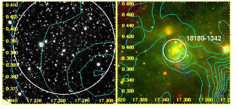
Figure 3: Four views of IRAS 18180-1342, like Figure 2. The guiding circle has a radius of $76\arcsec$. This object also falls within the partially covered GRS area. The blob has an angular diameter of $2\arcmin$, the largest apparent diameter of the near objects, but given its kinematic 2.0 kpc distance, it has a physical diameter of 1.2 pc.

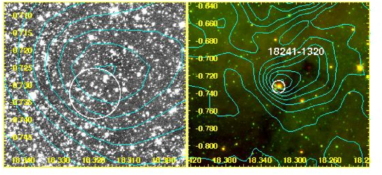
Figure 4: Four views of IRAS 18241-1320, like Figure 2. The guiding circle has a radius of $26\arcsec$. A rather small blob without any obvious clustering of stellar objects at the center of the blob. The blob is very likely, from spatial and velocity considerations, to be associated with the “clump” c7 in the cloud GRSMC G018.39-00.41 (Rathborne et al., 2009).

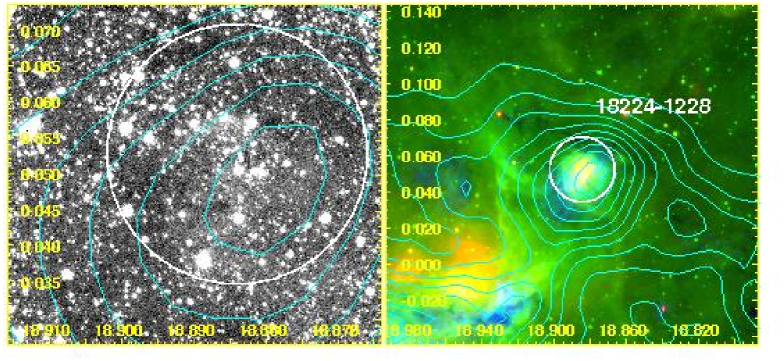
Figure 5: Four views of IRAS 18224-1228, like Figure 2. The guiding circle has a radius of $65\arcsec$. The largest (1.7 pc) and the most luminous ($2.7\times 10^{4}L_{\sun}$) of our near objects sits on the outskirts of the W39 complex. This blob is likely associated with “clump” c1 (another possibility is c2) in the cloud GRSMC G018.89+00.04. Looking at the position of the blob compared to BGPS, an association with BGPS G018.890+00.045 is likely (another possibility is BGPS G018.879+00.053).

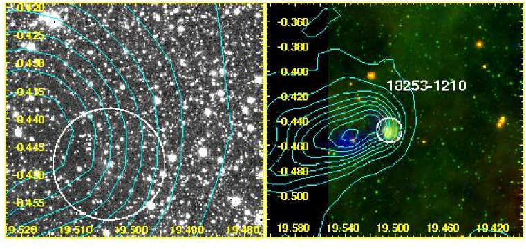
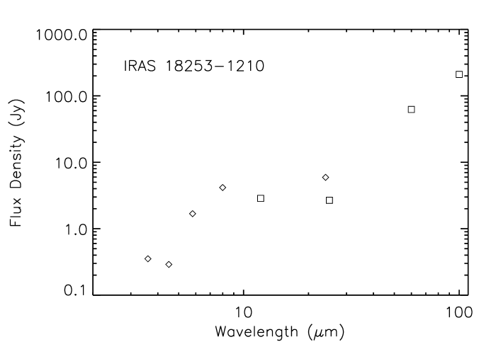
Figure 6: Four views of IRAS 18253-1210, like Figure 2. The guiding circle has a radius of $36\arcsec$. This $1\arcmin$ blob has a bow-shock like appearance. The molecular material indicated by the contours is associated with “clump” c1 in the cloud GRSMC G019.54-00.46. The IRAS blob is spatially associated with BGPS G019.507-00.447, while the position of maximum CO column density is spatially associated with BGPS G019.542-00.457.

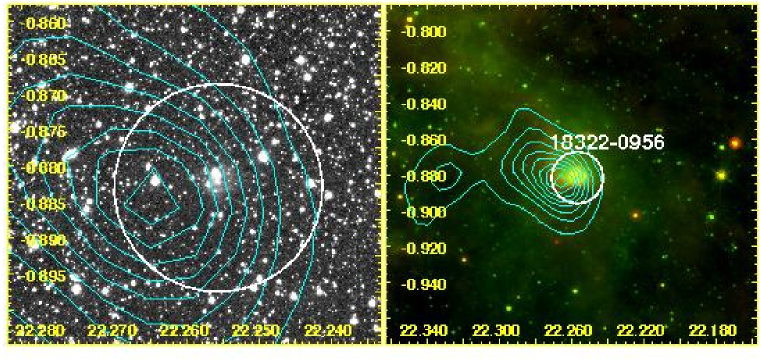
Figure 7: Four views of IRAS 18322-0956, like Figure 2. The guiding circle has a radius of $52\arcsec$. This is an isolated $0.6\arcmin$ blob, sitting on the edge of molecular material at 41.0 km s^-1. We note that it is possible that this source could be at a velocity of $\sim 65$ km s^-1, which would increase its physical diameter estimate by a factor of 1.4 and its luminosity estimate by a factor of 2.0.

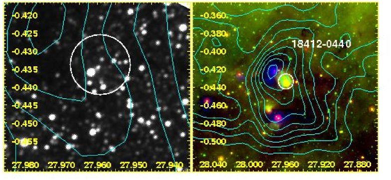
Figure 8: Four views of IRAS 18412-0440, like Figure 2. The guiding circle has a radius of $35\arcsec$. A $0.8\arcmin$ blob, clearly associated with IRDC G027.94-00.47 from Simon et al. (2006), which is seen to the left of the blob. Further associations are the “clump” c2 in GRSMC G027.99-0.46 and BGPS G027.972-00.422.

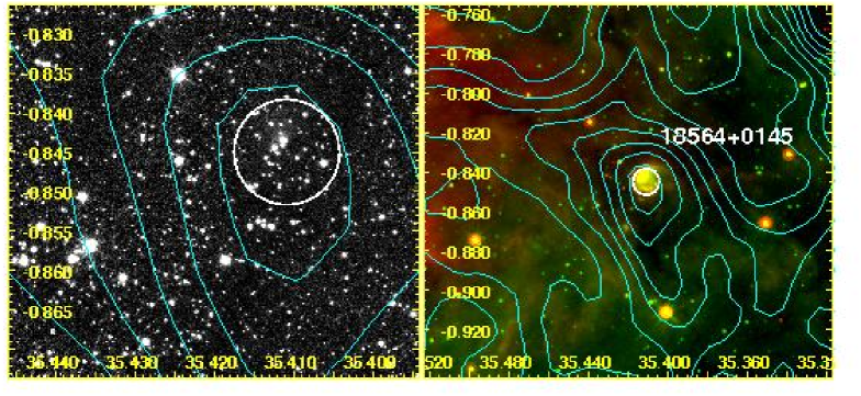
Figure 9: Four views of IRAS 18564+0145, like Figure 2. The guiding circle has a radius of $24\arcsec$. This $0.7\arcmin$ blob sits on CO that can be seen as dark absorption features in the 8.0 $\micron$ emission. The molecular material is likely referenced as “clump” c1 in GRSMC G035.59-00.91.

Figure 11: Figure showing the integrated flux density of IRAS 18180-1342 as a function of aperture radius at each of the four IRAC and the MIPS 24 $\micron$ bandpasses. The radial profiles are similar in each bandpass. The 8.0 and 24 $\micron$ flux densities asymptotically approach $\sim 42$ and $\sim 50$ Jy at a radius of $120\arcsec$. The chosen aperture radius of $76\arcsec$ is indicated by the dashed line and encompasses about half of this total.

Figure 13: Robitaille et al. (2006) model YSO luminosities of a range of Stage II objects as a function of stellar mass. The $L_{\mathrm{IR}}$ range found in Section 4.1, $10^{3}$ to $10^{4}$ L_☉, corresponds roughly to $\sim 4-10$ M_☉ YSOs, i.e., intermediate-mass.

Figure 20: (Left) Luminosity versus associated mass. (Right) Luminosity versus the peak mass column density, traced by millimeter-wave continuum. IM SFRs (15 objects) are diamonds. UCH II regions (33 objects) are crosses. The scale on the right is spectral type of a single class V star.

References

- Aguirre et al. (2009) Aguirre, J., et al. 2009, ApJ, submitted
- Barnes & Myers (1993) Barnes, P. J., & Myers, P. C. 1993, in ASP Conf. Ser. 35, Massive Stars: Their Lives in the Interstellar Medium, ed. J. P. Cassinelli & E. B. Churchwell (San Francisco, CA: ASP), 102
- Benjamin et al. (2003) Benjamin, R. A., et al. 2003, PASP, 115, 953
- Bonatto et al. (2006) Bonatto, C., Santos, J. F. C., Jr., & Bica, E. 2006, A&A, 445, 567
- Carey et al. (2005) Carey, S. J., et al. 2005, BAAS, 37, 1252
- Chapin et al. (2008) Chapin, E. L., et al. 2008, ApJ, 681, 428
- Chini et al. (1987) Chini, R., Kruegel, E., & Wargau, W. 1987, A&A, 181, 378
- Condon et al. (1998) Condon, J. J., Cotton, W. D., Greisen, E. W., Yin, Q. F., Perley, R. A., Taylor, G. B., & Broderick, J. J. 1998, AJ, 115, 1693
- Clemens (1985) Clemens, D. P. 1985, ApJ, 295, 422
- Deharveng et al. (2005) Deharveng, L., Zavagno, A., & Caplan, J. 2005, A&A, 433, 565
- Diaz-Miller et al. (1998) Diaz-Miller, R. I., Franco, J., & Shore, S. N. 1998, ApJ, 501, 192
- Emerson (1988) Emerson, J. P. 1988, in NATO ASIC Proc. 241: Formation and Evolution of Low Mass Stars, ed. A. K. Dupree & M. T. V. T. Lago (Dordrecht: Kluwer), 193
- Engelbracht et al. (2007) Engelbracht, C. W., et al. 2007, PASP, 119, 994
- Fazio et al. (2004) Fazio, G. G., et al. 2004, ApJS, 154, 10
- Fich & Terebey (1996) Fich, M., & Terebey, S. 1996, ApJ, 472, 624
- Giard et al. (1994) Giard, M., Bernard, J. P., Lacombe, F., Normand, P., & Rouan, D. 1994, A&A, 291, 239
- Hughes & MacLeod (1989) Hughes, V. A., & MacLeod, G. C. 1989, AJ, 97, 786
- Jackson et al. (2006) Jackson, J. M., et al. 2006, ApJS, 163, 145
- Kauffmann et al. (2008) Kauffmann, J., Bertoldi, F., Bourke, T. L., Evans, N. J., II, & Lee, C. W. 2008, A&A, 487, 993
- Kerton (2000) Kerton, C. R. 2000, Ph.D. Thesis, Univ. Toronto
- Kerton (2002) Kerton, C. R. 2002, AJ, 124, 3449
- Krumholz & McKee (2005) Krumholz, M. R., & McKee, C. F. 2005, ApJ, 630, 250
- Krumholz & McKee (2008) Krumholz, M. R., & McKee, C. F. 2008, Nature, 451, 1082
- Kuchar & Clark (1997) Kuchar, T. A., & Clark, F. O. 1997, ApJ, 488, 224
- Kwok et al. (1997) Kwok, S., Volk, K., & Bidelman, W. P. 1997, ApJS, 112, 557
- Lawrence et al. (2007) Lawrence, A., et al. 2007, MNRAS, 379, 1599
- Levine et al. (2008) Levine, E. S., Heiles, C., & Blitz, L. 2008, ApJ, 679, 1288
- Pandian & Goldsmith (2007) Pandian, J. D., & Goldsmith, P. F. 2007, ApJ, 669, 435
- Pandian et al. (2009) Pandian, J. D., Menten, K. M., & Goldsmith, P. F. 2009, ApJ, 706, 1609
- Pestalozzi et al. (2005) Pestalozzi, M. R., Minier, V., & Booth, R. S. 2005, A&A, 432, 737
- Rathborne et al. (2009) Rathborne, J. M., Johnson, A. M., Jackson, J. M., Shah, R. Y., & Simon, R. 2009, ApJS, 182, 131
- Reach et al. (2005) Reach, W. T., et al. 2005, PASP, 117, 978
- Rieke et al. (2004) Rieke, G. H., et al. 2004, ApJS, 154, 25
- Robitaille et al. (2006) Robitaille, T. P., Whitney, B. A., Indebetouw, R., Wood, K., & Denzmore, P. 2006, ApJS, 167, 256
- Rohlfs & Wilson (2004) Rohlfs, K., & Wilson, T. L. 2004, Tools of Radio Astronomy (4th ed.; New York: Springer)
- Roman-Duval et al. (2009) Roman-Duval, J., Jackson, J. M., Heyer, M., Johnson, A., Rathborne, J., Shah, R., & Simon, R. 2009, ApJ, 699, 1153
- Rosolowsky et al. (2010) Rosolowsky, E., et al. 2010, ApJS, 188, 123
- Rudolph et al. (1996) Rudolph, A. L., Brand, J., de Geus, E. J., & Wouterloot, J. G. A. 1996, ApJ, 458, 653
- Schaerer & de Koter (1997) Schaerer, D., & de Koter, A. 1997, A&A, 322, 598
- Simon et al. (2001) Simon, R., Jackson, J. M., Clemens, D. P., Bania, T. M., & Heyer, M. H. 2001, ApJ, 551, 747
- Simon et al. (2006) Simon, R., Rathborne, J. M., Shah, R. Y., Jackson, J. M., & Chambers, E. T. 2006, ApJ, 653, 1325
- Szymczak et al. (2000) Szymczak, M., Hrynek, G., & Kus, A. J. 2000, A&AS, 143, 269
- Walker et al. (1989) Walker, H. J., Volk, K., Wainscoat, R. J., Schwartz, D. E., & Cohen, M. 1989, AJ, 98, 2163
- Warren et al. (2007) Warren, S. J., et al. 2007, arXiv:astro-ph/0703037
- Weintraub (1990) Weintraub, D. A. 1990, ApJS, 74, 575
- Wood & Churchwell (1989a) Wood, D. O. S., & Churchwell, E. 1989a, ApJS, 69, 831
- Wood & Churchwell (1989b) Wood, D. O. S., & Churchwell, E. 1989b, ApJ, 340, 265
- Zinnecker & Yorke (2007) Zinnecker, H. & Yorke, H. W. 2007, ARA&A, 45, 481