A High Signal to Noise Map of the Sunyaev-Zel’dovich increment at 1.1 mm wavelength in Abell 1835

Abstract

We present an analysis of an 8 arcminute diameter map of the area around the galaxy cluster Abell 1835 from jiggle map observations at a wavelength of 1.1 mm using the Bolometric Camera (Bolocam) mounted on the Caltech Submillimeter Observatory (CSO). The data is well described by a model including an extended Sunyaev-Zel’dovich (SZ) signal from the cluster gas plus emission from two bright background submm galaxies magnified by the gravitational lensing of the cluster. The best-fit values for the central Compton value for the cluster and the fluxes of the two main point sources in the field: SMM J140104+0252, and SMM J14009+0252 are found to be $y_{0}=(4.34\pm 0.52\pm 0.69)\times 10^{-4}$, 6.5$\pm{2.0}\pm 0.7$ mJy and 11.3$\pm{1.9}\pm 1.1$ mJy, where the first error represents the statistical measurement error and the second error represents the estimated systematic error in the result. This measurement assumes the presence of dust emission from the cluster’s central cD galaxy of $1.8\pm 0.5$ mJy, based on higher frequency observations of Abell 1835. The cluster image represents one of the highest-significance SZ detections of a cluster in the positive region of the thermal SZ spectrum to date. The inferred central intensity is compared to other SZ measurements of Abell 1835 and this collection of results is used to obtain values for $y_{0}=(3.60\pm 0.24)\times 10^{-4}$ and the cluster peculiar velocity $v_{z}=-226\pm 275$ km/s.

1 Introduction

The Sunyaev Zel’dovich (SZ) effect (Sunyeav & Zel’dovich, 1970) is the redistribution of energy in the Cosmic Microwave Background (CMB) spectrum due to interations between CMB photons and hot electrons along the line of sight between the surface of last scattering and an observer. The main source for the SZ effect is from the hot gas that exists in the intra-cluster medium (ICM) of massive galaxy clusters (Birkinshaw, 1999; Carlstrom, Holder & Reese, 2002; Rephaeli, Sadeh & Shimon, 2006). The SZ actually comprises two effects. The thermal effect consists of a dimming or decrement in the apparent brightness of the CMB towards a galaxy cluster at low frequencies and a corresponding brightening or increment at high frequencies with the null crossover point at approximately 215 GHz. The kinematic effect has the spectral dependence of a standard temperature shift in the CMB which has the same sign at all frequencies. The two effects can therefore be distinguished from each other with measurements at multiple frequencies.

Measurements of the amplitude of the SZ thermal distortion towards a cluster can be combined with measurements of the X-ray emission to determine the angular diameter distance, $d_{A}$, whose value depends on cosmology (Birkinshaw, Hughes & Arnaud, 1991). Estimates of the Hubble constant have been made using this technique for a number of clusters (e.g. Jones (1995); Grainge (1996); Holzapfel et al. (1997); Tsuboi et al. (1998); Mauskopf et al. (2000); Reese (2003); Battistelli et al. (2003); Udomprasert et al. (2004)) and can be used to constrain cosmological models. In addition, because the SZ surface brightness for a cluster with a given mass is almost independent of redshift, SZ surveys can give information about the evolution of the number counts of clusters vs. redshift. This depends strongly on the evolution of the so-called dark energy or cosmological constant and therefore SZ surveys have been identified as one of the key probes of the nature of dark energy (e.g. Diego et al. (2002); Weller, Bettye & Kneissl (2002); DeDeo, Spergel & Trac (2005); Albrecht et al. (2006); Bhattacharya & Kosowsky (2007)). A number of dedicated SZ surveys are already producing results, in particular the Atacama Cosmology Telescope (ACT) and the South Polar Telescope (SPT) (Plagge et al., 2009; Hincks et al., 2009; High et al., 2010).

Most of the SZ detections reported to date have been made at low frequencies corresponding to the SZ decrement. Follow-up photometric or spectroscopic measurements of known clusters at higher frequencies would significantly improve the precision in the measurement of the kinematic SZ effect as well as constraining possible contamination in the low frequency data. Measurements at high frequencies corresponding to the SZ increment suffer from confusion from emission from dusty galaxies, including background high redshift galaxies amplified by the gravitational lensing of the cluster as well as increased atmospheric contamination from ground-based telescopes. Accurate measurement of the SZ increment requires a combination of angular resolution sufficient to resolve and remove point sources combined with high sensitivity and control of systematics necessary to detect the more diffuse SZ signal.

This paper presents analysis of observations of the galaxy cluster Abell 1835 using the Bolometric Camera (Bolocam) mounted on the Caltech Submillimeter Observatory (CSO), situated on the summit of Mauna Kea, Hawaii. We also compare the results of this analysis with other sets of data taken at different wavelengths. Abell 1835 is one of the most luminous clusters observed in the ROSAT catalogue and is well-known as a cooling core cluster. It is also known to contain two lensed sub-mm point sources, SMM J14009+0252 and SMM J140104+0252 (see e.g. Ivison et al. (2000); Zemcov et al. (2007)).

The paper is organized as follows: Section 2 describes the observations with the Bolocam instrument; Section 3 describes the analysis pipeline developed for processing the data; Section 4 describes the modelling of the data and the determination of the characteristic parameters of the model (as well as the errors in their values), and Section 5 discusses the results of the analysis of the Bolocam data and their combination with other literature results.

2 Observations

The data used in this work represents approximately 12.5 hours of observations taken over the course of five nights at the end of January/ beginning of February 2006. The observations were made with Bolocam operating at 1.1 mm (275 GHz).

Bolocam consists of an array of 105 operational neutron-transmutation-doped (NTD) Germanium spiderweb bolometers, capable of observing at 1.1 mm or 2.1 mm (Glenn et al., 1998; Haig et al., 2004). The system is cooled to 270 mK to allow the array to operate close to the photon background limit at 1.1 mm. The Bolocam array has a field of view of approximately 8 arcmin, and the beam FWHM is $\sim$ 30” at 1.1 mm (and $\sim$ 60” at 2.1 mm).

The detector is mounted at the Cassegrain focus of the Leighton telescope - the 10.4 m CSO dish. The principal science targets for the instrument include star forming regions in the galaxy, blank-field surveys for dusty extragalactic point sources; blank field SZ cluster surveys, and pointed observations of galaxy clusters.

Observations by Bolocam incorporate a number of different scan strategies. The majority of observations use raster scanning or lissajous scanning where the entire telescope is constantly in motion modulating the array position on the sky.

The data presented in this paper was taken using jiggle mapping. Jiggle mapping uses a combination of ’chopping’ the secondary mirror during observations, i.e. switching the secondary from side-to-side, and ’nodding’ the telescope, i.e. changing the position of the telescope during a scan. The beam moves from being ’on-source’ (imaging the region of the target and chopping away from it), to ’off-source’ (imaging a nearby region of blank sky and chopping onto the target), then returns to being on-source once again (see Fig. 1).

Figure 1: Nodding and acquisition pattern (top). A nod position of +1 implies the telescope is on-source, whereas nod position -1 is when the telescope is off-source. The pattern is a combination of acquisition and positional data, so that where the pattern falls to zero this reflects where the telescope is not acquiring data (usually while the dish is moving to a different location on the sky). A sample of the raw data demonstrating the chopping is also given (bottom).

Jiggle mapping is a means of removing sky background from data, and works by differencing signal from so-called ’target’ and ’reference’ beams (centered on the science target and a region of ’blank’ sky, respectively). These beams are also referred to as ’on’ and ’off’ beams. While jiggle-mapping is an efficient method of subtracting sky-noise, care has to be taken to ensure that the chop ’throw’ (i.e. the maximum angular dispacement of the secondary during the chop) is large enough that the off beam does not pick up signal from the source itself (subject to mechanical limitations). For this reason, jiggle-mapping is not always suitable for imaging extended sources, but is good for observing point sources.

The chop frequency for this data set was 2.25 Hz, giving a chop period of $\sim$ 0.44 s (compared to a sampling rate of 0.02 s). The chop throw was 90”, while the displacement between on and off beams during the nods was 2.5’. The telescope typically remained in the ’on’ or ’off’ phase for periods of approximately 10 seconds.

The full set of data consisted of fifteen individual sets of observations of approximately 50 minutes each. The observations were separated by shorter observations of planets and other sources with known position and flux, which could be used for the calibration and pointing.

3 Pipeline development

Because jiggle-mapping is a relatively new strategy for Bolocam, there was initially no pipeline in place to analyse the raw data. An independent pipeline was written specifically for this observing mode.

In its original form, the time-stream data had been sliced (i.e. separated into individual data-vectors representing the signal from individual bolometers during specific observations), but no other processing had taken place. The pipeline for jiggle data includes the following elements:

1. Initial cleaning to remove obvious sources of noise using average subtraction;

2. Identifying the nodding sequence;

3. Identifying phase differences between the signal from the chop control and the data (due, for example, to differences in timing between the telescope clock and those in the telescope control terminals);

4. Deconvolving the data for each nod position (’removing’ the chopping);

5. Extracting the signal (differencing the deconvolved signal from the nod positions);

6. Calculating errors for the signals;

7. Determining pointing corrections for each map and hence reconstructing the directional information for each map;

8. Calibrating the maps;

9. Saving the deconvolved datasets,

10. Coadding maps from individual observations.

3.1 Deconvolving

We deconvolve the chopped data using a fit to the time stream signal monitoring the chopper position corrected for a phase difference between the chopper data and bolometer data. If the signal being detected by an individual bolometer is modulated by the chopping according to:

$$\mathrm{F}(t)=\mathrm{F}_{\mathrm{s}}\sin[\nu_{\mathrm{c}}t+\phi_{\mathrm{c}}]$$ (1)

where $\mathrm{F}(t)$ is the time($t$)-varying flux received by the bolometer, $\mathrm{F}_{\mathrm{s}}$ is the flux of the source, $\nu_{\mathrm{c}}$ is the chop frequency, $\phi_{\mathrm{c}}$ is the chop phase, one can then multiply this by a fit and integrate according to:

$$\mathrm{S}(t)={\int\mathrm{F}(t)\sin[\nu_{\mathrm{f}}t+\phi_{\mathrm{f}}]\mathrm{d}t\over\int\sin^{2}[\nu_{\mathrm{f}}t+\phi_{\mathrm{f}}]\mathrm{d}t}$$ (2)

where $\nu_{\mathrm{f}}$ is the fit frequency, $\phi_{\mathrm{f}}$ is the fit phase.

With an accurate enough fit $(\nu_{\mathrm{f}}\sim\nu_{\mathrm{c}}$, $\phi_{\mathrm{f}}\sim\phi_{\mathrm{c}}$), therefore, $S(t)\rightarrow\mathrm{F}_{\mathrm{s}}$. The value of $\nu_{\mathrm{f}}$ is measured from a fit to the chopper data, and the integration needs to be over a complete number of chopping cycles to avoid spurious signal being introduced into the maps.

3.2 Pointing

The individual detector pointing data was reconstructed in three stages. First a map was made of the deconvolved data. The directional information was taken from the time-streams of azimuth and elevation stored with the raw data (converted to ra and dec) and previously determined offsets (to convert the values stored at the telescope with the actual azimuth and elevation of the centre of the telescope beam) were added. The mean of these values were compared to the recorded position of the source to obtain a ’mean’ offset.

The directional information for the map was then reconstructed to include the mean offsets. The location of the centre of emission for the source in the map was determined using a simple $\chi^{2}$ fit of the data immediately around the cluster to a gaussian. This position was then compared once more with the source values to determine a ’fine’ offset.

The directional information was then undated again to include both the mean and fine offsets.

3.3 Calibration

The calibration for Bolocam is determined using the resistances of the bolometers as determined by the dc level of the lock-in amplifier output signal, which is expected to be directly related to the flux calibration for a set of observations (see Laurent et al. (2005)). If observations can be made of a number of sources of known flux at different levels of sky loading a plot can be made of the dc level against calibration factor. We fit a second-order polynomial to the measured calibration points to extend the calibration to the full range of observation conditions. In this way, we can determine the correct calibration for an observation within an appropriate range of dc level.

These calibration curves are not expected to change significantly over time. However, given that the previous set of data was taken in May 2004, using a different scanning technique, we performed a full set of calibration observations roughly every 20 minutes during the science observations. These calibration sources were chosen to be close to the science observation target and included: 0420m014; 0923p392$\_$4cp39.25; 1334$-$127, and 3c371. The resulting calibration curve is given in Fig. 2.

The observations of the calibrators agree reasonably well with the May 2004 calibration curve. The point sources used in the plot were all secondary sources and as a result it was not clear how precise or stable their fluxes would be. Given this, the deviations between the old calibration curve and the sources were not considered to be great enough to warrant revising the calibration values and adopting a new functional form for the calibration, and the May 2004 calibration was used throughout.

Figure 2: Calibration data. The May 2004 calibration curve is shown as the solid line. The error bars in this figure are statistical errors from the measured data. They do not, therefore, include intrinsic uncertainty in the source brightness. The data does not deviate substantially from the May 2004 curve. Legend: Vertical crosses: 0420m014; open triangles: 0923p392$\_$4cp39.25; open diamonds: 1334-127, open squares: 3c371.

4 Modelling and parameter estimation

Once maps had been made of the individual observations, they were coadded to produce a single image of Abell 1835 which was then also convolved with a Gaussian PSF with FWHM $\sim$ 30.6“ , corresponding to the best-fitting Gaussian to the Bolocam beam (Fig. 3).

Figure 3: (Top left) S/N map of the raw data, convolved with the Bolocam beam; (top right) 3-parameter fit ($\beta=0.69$, $\theta_{c}=33.6^{\prime\prime}$) S/N map convolved with the Bolocam beam, (bottom) Map of residuals, formed by taking the difference between the convolved model and data S/N maps.

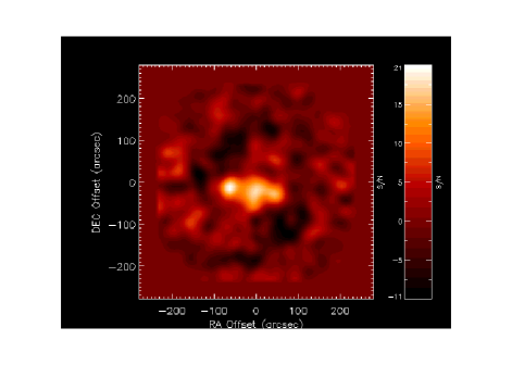
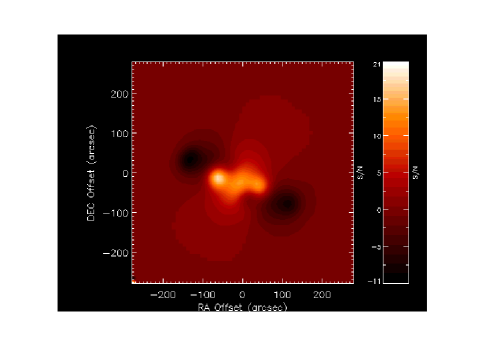
A model was produced to simulate the observations and derive estimates of the fluxes of the sources. Fig. 3 clearly shows the two point sources arranged on either side of the emission from the cluster (which is assumed to be entirely signal from the SZ). These point sources have been detected previously at 850 $\mu$m using the Submillimeter Common User Bolometer Array (SCUBA) on the James Clerk Maxwell Telescope (JCMT) (Zemcov et al., 2007) as well as by Ivison et al. (2000). The characteristics of these point sources, reported by Zemcov et al. (2007) are given in Table 1.

Source id	ra (hh:mm:ss)	dec (dd:mm:ss)	850 $\mu$m Flux (mJy)	450 $\mu$m Flux (mJy)
SMM J14011+0252	14:01:04.7	+02:52:25	14.6$\pm$1.8	41.9$\pm$6.9
SMM J14009+0252	14:00:57.5	+02:52:49	15.6$\pm$1.9	32.7$\pm$8.9

Table 1: Point source positions and fluxes reproduced from Ivison et al. (2000)

The SZ emission from the galaxy cluster itself was modelled assuming that the signal was dominated by the thermal SZ and assuming an isothermal beta radial profile:

$$\mathcal{F}(\theta_{p})=\mathrm{\it}{A}\left(1+\frac{\theta_{p}}{\theta_{c}}\right)^{\left(\frac{1}{2}-\frac{3\beta}{2}\right)}$$ (3)

where $\mathcal{F}(\theta_{p})$ is the flux profile of the cluster as a function of projected angle $\theta_{p}$, $\theta_{c}$ and $\beta$ are fitting parameters $\mathrm{\it}{A}$ is a scaling parameter, defined by:

$$\mathrm{A}=\Delta\Omega\mathrm{I}_{\tiny{0}}\mathrm{y}_{0}\mathrm{g(x)}\times 10^{26}$$ (4)

Here: $\Delta\Omega$ is the solid angle of the pixels in the (model) map (the map was later convolved with the Bolocam beam such that the final flux measurements were given in flux/beam), $I_{0}=\frac{2h}{c^{2}}\left(\frac{k_{B}T_{CMB}}{h}\right)^{3}$, is the blackbody emission of the CMB at the redshift of the cluster, $\mathrm{y}_{0}$ is the so-called ’Compton parameter’ at the centre of the cluster (the Compton parameter in general, $\mathrm{y}$, can be characterised as:

$$\mathrm{y}=\int{\mathrm{n}_{e}\sigma_{T}\frac{\mathrm{k}_{B}\mathrm{T}_{e}}{\mathrm{m_{e}}\mathrm{c}^{2}}}\mathrm{dl}$$ (5)

where $\mathrm{n}_{e}$ and $\mathrm{T}_{e}$ are, respectively, the electron density and electron temperature along the line of sight), and $\mathrm{g(x)}$ is a function that depends on the dimensionless frequency at which the observations are being made, $\mathrm{x}=\frac{\mathrm{h}\nu}{\mathrm{k}_{B}\mathrm{T}_{\mathrm{CMB}}}$, as:

$$\mathrm{g(x)}=x^{4}\frac{\exp{x}}{(\exp{x}-1)^{2}}(x\coth{(x/2)}-4)$$ (6)

The temperature reported in the literature for Abell 1835 varies between approx. 8 - 10 keV (e.g. Allen & Fabian (1998); Peterson et al, (2001); Katayama & Hayashida (2004)). At these temperatures, relativistic corrections to the SZ can be on the order of $\sim$ 10$\%$ and have to be taken into account during the analysis. We used the corrections published by Itoh, Kohyama & Nozawa (1998), up to fifth order in $\theta$, where:

$$\mathrm{\theta}=\frac{\mathrm{k}_{B}\mathrm{T}_{e}}{\mathrm{m}_{e}\mathrm{c}^{2}}$$ (7)

An ideal sky model was produced including extended emission from the cluster and emission from the point sources at positions given by Zemcov et al. (2007). The free parameters of the model were the cluster geometry ($\theta_{c}$ and $\beta$); the comptonization ($y_{0}$), and the fluxes of the two point sources $\mathcal{F}_{1}$ and $\mathcal{F}_{2}$ (corresponding to SMM J0140104+0252 and SMM J14009+0252, respectively). For each set of parameters, we produced a high resolution map with pixel size of 1”. This map was then convolved with the Bolocam beam to produce a ’real-sky’ map of the cluster at the resolution of the telescope. This in turn was then ’observed’ by using the data ra and dec values to reproduce the effect of the jiggling, thereby producing a simulation of what we expect to observe given the assumed values of flux (for the point sources) and $\mathrm{y}_{0}$. Finally, the chopped map was rebinned to the same pixel size as the raw data maps. By comparing the maps corresponding to different values of the parameters with the data, we construct a multi-parameter likelihood space, which could be searched to extract best fitting models.

Values for these parameters were determined by searching for the set that minimized the $\chi^{2}$ value between the model map and the data map.

Generally, SZ observations are not able to constrain the parameters $\theta_{c}$ and $\beta$, since the resolution of such experiments is not accurate enough to constrain their values to a better degree of accuracy than equivalent X-ray (or other wavelength) measurements. Recently, however, computer simulations have suggested that using X-ray derived profiles for fitting SZ observations can lead to bias in the derived values of $\mathrm{y}$ (Hallman et al., 2007). Furthermore, the values of the profile parameters quoted in the literature can vary considerably (see, e.g. values reported in Jia et al. (2004); Peterson et al, (2001); Schmidt, Allen & Fabian (2001); Zemcov et al. (2007)).

In this work, therefore, a range of approaches have been adopted. Fits to $\mathrm{y}$, $\mathcal{F}_{1}$ and $\mathcal{F}_{2}$ were made using two different sets of values for $\theta_{c}$ and $\beta$ obtained using Chandra X-ray data and interferometric SZ data from the Owens Valley Radio Observatory (OVRO) and the Berkeley Illinois Maryland Association (BIMA), taken fromLaRoque et al. (2006).

The cores of galaxy clusters can exhibit sharp peaks in emission due to the presence of cooling flows, and for this reason a single isothermal beta model fit to all the X-ray data in a set of observations is not always suitable. LaRoque et al. (2006) use two different strategies to deal with this. In the first the X-ray data set is restricted to exclude the region within 100 kpc of the X-ray centre, and the profile parameters are then obtained by a joint fit to this X-ray data and the entire set of SZ data. It is possible to use the entire SZ dataset since SZ emission has a weaker dependence upon electron density than X-ray observations, and the SZ profile is not expected to be significantly affected by the presence of cooling flows. (Indeed in general, the SZ profile is less sensitive to the detailed physics in the cores of galaxy clusters (Motl et al., 2005).) In the second approach they employ a double-beta model which has been used to fit all the X-ray data in observations that include emission from cooling flows (see e.g. Mohr, Mathiesen & Evrard (1999)). LaRoque et al. (2006) also fit to the SZ data only (although this fit is really only to $\theta_{c}$ since the value of $\beta$ is fixed to the value obtained for the isothermal beta X-ray/ SZ fit).

For the purpose of this analysis the results from the isothermal beta fit to the restricted X-ray data and SZ data (hereafter LaRoque X-ray+SZ) and the fit to the SZ data (hereafter LaRoque SZ only) were used. The values of $\theta$ and $\beta$ they obtain for these fits are, for the combined X-ray and SZ data: $\beta=0.69$, $\theta_{c}=33.6^{\prime\prime}$, and for the SZ-only data: $\beta=0.70$, $\theta_{c}=50.1^{\prime\prime}$.

It was decided, therefore, to fit the data from the Bolocam observations with five combinations of profile parameters: $\beta=0.69$, $\theta_{c}=33.6^{\prime\prime}$; $\beta=0.69$, $\theta_{c}=50.1^{\prime\prime}$; $\beta=0.69$; $\theta=33.6^{\prime\prime}$, and $\theta=50.1^{\prime\prime}$, where the other parameters are fitted for in each situation.

The goodness of fit for a particular set of parameters was evaluated using a $\chi^{2}$ test. The value for $\chi^{2}$ for a given model was defined simply as:

$$\chi^{2}=\displaystyle\sum_{i}{\frac{(\mathrm{data}_{i}-\mathrm{model}_{i})^{2}}{\sigma_{i}}}$$ (8)

where $\mathrm{data}_{i}$ denotes the signal in the i’th pixel of the data map, $\mathrm{model}_{i}$ represents the signal in the i’th pixel of the model map, and $\sigma_{i}$ is the noise in the i’th pixel of the noise map. The best fitting parameters for a given analysis run were, therefore, those that minimized this value of $\chi^{2}$.

For the cases in which there were four free parameters to be searched through, the individual searches took a long time to process. The general method of locating a minimum was to sample the parameter space between ’reasonable’ limits, locate a minimum and examine variation in the $\chi^{2}$ values for each parameter while keeping the other parameters fixed. This variation was in general smooth and reasonably quadratic, so that the first derivatives of the variation was typically linear. This could easily be fit and an estimate made of where the first derivative was zero. The limits of the search were then reset to centre on the new approximation for the minimum and the process repeated until the new estimates of the minima were similar (within some tolerance) to the previous ones. This approach allowed the minimum values to be located within a reasonable amount of time.

Errors on the values of the fit parameters were found by deriving the inverse of the Fisher matrix for the observations and evaluating its diagonal elements. For parameters with a gaussian distribution, the Fisher matrix ${\it F}_{ij}$ is given by:

$${\it F}_{ij}=\frac{1}{2}\left(\frac{\partial^{2}\chi^{2}}{\partial{p_{i}}\partial{p_{j}}}\right)$$ (9)

where $p_{i}$ represents the vector of parameters being fit, and the second-order differential is evaluated at the value of $p$ at which the $\chi^{2}$ value is minimized.

This kind of analysis relies on there being no covariance between different pixels in the data maps. The level of covariance is expected to be low due to the chopping, and because the only cleaning of the data involves an average subtraction. This should introduce less pixel to pixel covariance than other cleaning methods. Jacknife maps were also made to check these assumptions, and were found to show no evidence for significant levels of covariance.

The components of ${\it F}_{ij}$ were evaluated using a finite difference scheme and arrays of $\chi^{2}$ values around the minimum values. The $\chi^{2}$ values were obtained by varying the fit parameters as well as the position of the central emission. The results of this analysis are shown in Table 2.

$\beta_{model}$	0.69	0.69	0.69	–	–	0.69 (p)
$\left(\theta_{c}\right)_{model}$ (′′)	33.6	50.1	–	33.6	50.1	33.6 (p)
$\mathcal{F}_{1}$ (mJy)	6.48$\pm{2.00}$	6.22$\pm{2.08}$	7.16$\pm{1.88}$	7.09$\pm{1.89}$	7.17$\pm{1.84}$	6.48$\pm{2.00}$
$\mathcal{F}_{2}$ (mJy)	11.32$\pm{1.92}$	10.90$\pm{1.98}$	11.98$\pm{1.79}$	12.38$\pm{1.82}$	12.18$\pm{1.77}$	11.32$\pm{1.92}$
$\mathrm{y}_{0}\times{10^{-4}}$	(4.68$\pm{0.48}$)	(4.43$\pm{0.49}$)	(6.52$\pm{0.64}$)	(4.85$\pm{0.47}$)	(4.19$\pm{0.40}$)	(4.34$\pm 0.52$)
$\beta$	0.69	0.69	0.69	$1.20\pm{0.2}$	$1.60\pm{0.2}$	0.69
$\theta_{\mathrm{c}}$ (′′)	33.6	50.1	$14.7^{+2.4}_{-2.2}$	33.6	50.1	33.6
ra offset (′′)	1.8	1.9	2.1	2.1	2.0	2.0
dec offset (′′)	3.6	3.9	2.6	2.8	2.5	3.4
$\chi^{2}$	3066	3079	3058	3056	3054	3062

Table 2: Parameter estimates (1 mm Bolocam observations) and $\chi^{2}$ values; Number of degrees of freedom = 3013. (p) denotes that the model included a 1.8 mJy point source at the cluster centre.

5 Results

The results of Table 2 shows that the 4-parameter fit with $\theta_{c}=50.1^{\prime\prime}$ gives the best ($\chi^{2}$) value. The best fit values of the central Compton parameter as well as the fluxes of the point sources are, therefore, found to be: $y_{0}=(4.19\pm 0.48)\times 10^{-4}$; 7.17$\pm$1.84 mJy, and 12.18$\pm$1.77 mJy respectively. The errors on the values of $y_{0}$ in Table 2 include statistical errors as well as errors due to pointing and uncertainty in the model parameters. They do not include systematic errors (e.g. due to dust contamination, kinetic SZ, etc.). The systematic uncertainties are discussed in greater detail below.

The value of $\beta$ for our best fit model is substantially different from values quoted by other groups, who use X-ray data with much better resolution to calculate their profile parameters. It is common practice to treat these measurements as more reliable in determining cluster profile parameters (although see Hallman et al. (2007)). Furthermore, since a comparison of our data to that of other groups was planned, the cluster model for which intensity measurements were being compared had to be the same. For these reasons, it was decided that, in forming the comparison with data at other frequencies, the results for the more ’canonical’ values the profile parameters should be used. Of the two fits with more typical profile parameters, the $\beta=0.69$, $\theta_{c}=33.6^{\prime\prime}$ fit has the lower $\chi^{2}$ value, and is the model used for the spectral fitting.

Additional sources in the field

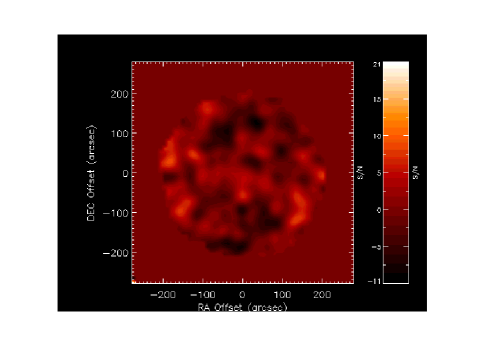
In order to reliably simulate a series of chopped observations, all sources in the field need to be accounted for. The $\beta=0.69$, $\theta_{c}=33.6^{\prime\prime}$ fit model is also shown in Fig. 3, convolved with the Bolocam beam. The final map in Fig. 3 displays the difference between the model map and the raw data, convolved with the Bolocam beam to emphasize any differences between them. The difference map appears to indicate that the cluster signal and the point sources have been removed effectively and that, therefore, the model is a reasonable simulation of the data. The signal at the edge of the field is mostly spurious. It could be suggested that there is a $\sim$ 3-$\sigma$ detection (in the raw map) of a point source just below centre of the image field, but there are no obvious listed sources located at the position of the candidate detection, and it appears that most likely to be a spurious feature of the noise.

Using noise maps calculated in the analysis, it was possible to form a histogram of the difference between the S/N data map and the simulated map (see Fig. 4, where the data is plotted on logarithmic axes to determine whether there was significant deviation between the residuals and the fit toward the limits of the data). The Gaussian form of the histogram (quadratic in Fig. 4) is consistent with the residual signal being dominated by noise, rather than other point sources. The histogram was fit with a Gaussian, and the best fit has a standard deviation close to 1.0, indicating that the noise had been correctly estimated. There may be some suggestion of deviation in the high S/N region between the histogram and the fit, but this is attributed to regions of lower coverage in the outer sections of the map, and not believed to represent a real excess of sources.

Figure 4: Signal to noise histogram of the residual map obtained by subtracting the best fit model from the data, plotted on logarithmic scales. The Gaussian best fit to the histogram (the solid line in the log plot) has $\sigma=1.01$

Dust Contribution

At longer wavelengths the contribution from dust emission is expected to become more important and is a source of confusion. The literature does not provide an entirely consistent view of whether or not Abell 1835 has significant dust emission. While the cluster’s brightest cluster galaxy (BCG) exhibits significant CO emission which is believed to trace dust, it would be expected that the dust emission would be extremely bright at 450 $\mu$m. There are a limited number of results in the literature that report emission from Abell 1835 at 450 $\mu$m. Ivison et al. (2000) and Edge et al. (1999) report strong emission, consistent with a significant dust contribution, whereas the 450 $\mu$m result given in Zemcov et al. (2007) of -2 $\pm$13 mJy is consistent with there being no emission from the cluster at this wavelength.

Assuming a ’worst case’ scenario , however, in which the emission reported by Ivison et al. (2000) at 450 and 850 $\mu$m are assumed to be correct, and all the signal at these wavelengths is attributable to the cD galaxy, a model can be formed of the dust emission using a greybody spectrum, assuming a dust temperature $\sim$ 30 K and an emissivity which varies as $\nu^{1.5}$. The flux of the cD galaxy at 1.1mm using this model is expected to be $\sim 1.8\pm 0.5$ mJy. This value is consistent with the SED produced for Abell 1835’s BCG reported by Egami et al. (2006). Introducing a point source into the cluster model at the X-ray centre and then marginalizing again over values of $y_{0}$, we obtain a best fit value for $y_{0}$ of $(4.34\pm 0.52)\times 10^{-4}$, with a $\chi^{2}$ value of $\sim$ 3062.

Figure 5: The SZ spectrum of Abell 1835. The 30 GHz results (open triangle, $x\sim 0.5$) are taken from.LaRoque, et al. (2006). The points at 142 and 221 GHz (open diamonds) are from Mauskopf, et al. (2000), while the open square represents the results reported here. All points have been renormalised to the central intensity of the SZ effect for a cluster model with $\theta_{0}=33.6^{\prime\prime}$ and $\beta=0.69$. The line is the best fit SZ spectrum with $y_{0}=3.60\times 10^{-4}$ and $v_{z}=-226$ km/s.

Systematic errors	Error (as $\%$ of result)
Calibration	11.7
Kinematic effect	9.0
CMB confusion	1.0
Dusty galaxies	5.4
Dust emission	7.2
Effective temperature	${}^{+1.5}_{-2.6}$
Uncertainties in	0.6
King model parameters
Others (clumping, etc)	2
Pointing and model	0.52 mJy
error (incl. point
source
Total systematic	0.69 mJy
Total error	0.87 mJy

Table 3: Error budget for Abell 1835 observations

Other sources of error

Along with the dust contribution, it was important to account for other sources of error in the result. These are discussed individually below:

Calibration

We estimated the calibration error from the noise-weighted dispersion of the measured point fluxes relative to the May, 2004 model. This gives a calibration error of $\sim$ 10.6$\%$, which, when combined with a 5$\%$ error due to uncertainties in the Mars model that all the Bolocam fluxes are dependent on gave an overall calibration error of $\sim$ 11.7$\%$.

Kinematic effect

The kinematic SZ effect (see below) is due to the bulk motion of a cluster. In general, the kinematic effect is much less significant than the thermal effect that has been discussed so far. The bulk motion of clusters in a concordance cosmology predicts an rms peculiar velocity of around 300 km/s, but Mauskopf et al. (2000) obtain an estimate of the velocity of Abell 1835 of around 500 km/s. A velocity this high at 273 GHz produces a kinematic effect that is approxiamtely 9$\%$ of the thermal effect.

Confusion sources

The main sources of confusion in observations of the SZ effect include the CMB background and dusty galaxies. Typical CMB temperature anisotropy signals based on the current concordance model spectrum was simulated and ’observed’ using our scan strategy. These produced an rms equivalent to a 1.5$\%$ error in the measured cluster signal. Dusty galaxies at 1.1 mm contribute an rms signal of approximately 0.5 mJy (e.g. Blain (1998)), which corresponds to a 5.4$\%$ error in the measured cluster signal.

Physical model uncertainties

Other sources of error related to the parameters of the physical model of Abell 1835 itself. Uncertainties in the electron gas temperature of 10 - 15 $\%$ correspond to an error in the estimate of $y_{0}$ of up to $\sim$ 2.5$\%$. LaRoque et al. (2006) reports errors on the model parameters $\theta_{c}$ and $\beta$ of $\pm$1.0” n and $\sim$ 0.01, respectively. When these variations are introduced into the model to see what effect they have on the value of $y_{0}$ obtained by the fit, their effect is found to be small, and represent an uncertainty on the level of 0.6 $\%$ on the final result. Other potential sources of error include (e.g.) clumping in the cluster gas, but the SZ effect is relatively insensitive to the detailed physics of cluster gas, these effects were estimated as contributing no more than $\sim$ 2$\%$ to the final result.

A breakdown of the error budget for the observations presented here is given in Table 3.

$y_{0}$ estimates

The value of $y_{0}$ given by the 4 parameter fit means that the observations detect the cluster with a significance of 10.5$\sigma$. This is one of the highest significance detections of a cluster in the positive region of the SZ spectrum to date. A plot of the SZ spectrum of Abell 1835 based upon these values is given in Fig. 5. These values have were fitted with a spectrum that included kinetic and thermal effects (non-relativistic as well as relativistic). The kinetic effect follows the form:

$$I_{kinetic}=-\tau_{e}\beta h(x)$$ (10)

where $\tau$ is the optical depth of the cluster gas, given by $y_{0}\left(\frac{mc^{2}}{k_{B}T_{e}})\right)$, $\beta\equiv\frac{v_{z}}{c}$ (where $v_{z}$ is the peculiar velocity of the galaxy cluster), and $h(x)=x^{4}\frac{\exp{x}}{(\exp{x}-1)^{2}}$. The kinetic effect dominates the SZ spectrum around the null point ($\nu\sim 217$ GHz, x $\sim$ 1.9), but makes only a small contribution to the spectrum at frequencies above or below this.

The free parameters of the fit to the SZ spectrum were, therefore, $y_{0}$ (which characterizes the thermal SZ), and $v_{z}$ (which characterizes the kinetic effect). The values of these parameters that optimized the fit were found to be: $y_{0}=(3.60\pm 0.24)\times 10^{-4}$, and $v_{z}=-226\pm 275$ km/s. This is consistent with previous measurements of $v_{z}$ for Abell 1835 Benson et al. (2004); Mauskopf et al. (2000) and represents the most sensitive test for peculiar velocity in an individual galaxy cluster using the SZ effect to date.

6 Conclusions

The observation and analysis of 1.1 mm Bolocam jiggle-map data of Abell 1835, including details of the process of converting the raw data to maps of the cluster, have been discussed. A parameter search has been used to determine the best fit values of the central Compton parameter for the cluster and the fluxes for the point sources SMM J140104+0252 and SMM J14009+0252. These values are found to be $y_{0}=(4.68\pm 0.48\pm 0.82)\times 10^{-4}$, 6.5$\pm{2.0}$ mJy and 11.3$\pm{1.9}$ mJy, respectively with a statistical signal-to-noise of 10.5, 3.3 and 6.0 respectively. If the model is refined further to include a point source, representing dust emission from the cD galaxy in Abell 1835, the Compton parameter for the cluster is found to be $y_{0}=(4.34\pm 0.52\pm 0.69)\times 10^{-4}$ The value for $y_{0}$ was compared to other literature results and found to agree well. The SZ spectrum for Abell 1835, based upon these values for $y_{0}$ was fit with the full SZ form, including both thermal and kinetic effects and relativistic corrections up to 7th order. The values of $y_{0}$ and $v_{z}$ which optimized this fit were found to be $(3.60\pm 0.24)\times 10^{-4}$ and $-226\pm 275$ km/s, which are both in agreement with previous literature results. It is also concluded that, in order to better evaluate the contamination from dust and accurately characterize the spectrum of point sources in the same field as SZ clusters more results need to be obtained at shorter wavelengths in order to obtain more a detailed spectral energy distribution.

References

- Albrecht et al. (2006) Albrecht A., Bernstein G., Cahn R. et al., 2006, preprint(astro-ph/0609591)
- Allen & Fabian (1998) Allen S. W., Fabian A. C., MNRAS, 297, L57, 1998
- Battistelli et al. (2003) Battistelli E. S., De Petris M., Lamagna L. et al., 2003, preprint(astro-ph/0303587)
- Benson et al. (2004) Benson B. A., Church S. E., Ade P. A. R., Bock J. J., Ganga K. M., Henson C. N., Thompson K. L., 2004, ApJ, 617, 829
- Bhattacharya & Kosowsky (2007) Bhattacharya S., Kosowsky A., 2007, preprint (astro-ph/0712.0034)
- Birkinshaw, Hughes & Arnaud (1991) Birkinshaw M., Hughes J. P., Arnaud K. A., 1991, ApJ, 376, 466
- Birkinshaw (1999) Birkinshaw M., 1999, Phys. Rep., 310, 97
- Blain (1998) Blain A. W., 1998, MNRAS, 297, 502
- Carlstrom, Holder & Reese (2002) Carlstrom J. E., Holder G. P., Reese E. D., 2002, ARA&A, 40, 643
- DeDeo, Spergel & Trac (2005) DeDeo S., Spergel D. N., Trac H., 2005, preprint(astro-ph/0511060)
- Diego et al. (2002) Diego J. M., Martinez-Gonzalez E., Sanz J. L., Benitez, Silk J., 2002, MNRAS, 331, 556
- Edge et al. (1999) Edge A. C., Ivinson R. J., Smail I., Blain A. W., Kneib J. -P., 1999, MNRAS, 306, 599
- Egami et al. (2006) Egami E., Misselt K. A., Rieke G. H. et al., 2006, ApJ, 647, 922
- Glenn et al. (1998) Glenn J., Bock J. J., Chattopadhyay G. et al., 1998 in, Proc. SPIE, 3357, 326
- Grainge (1996) Grainge K., 1996, PhD thesis, Cambridge University
- Grego et al. (2001) Grego L., Carlstrom J. E., Reese E. D., Holder G. P., Holzapfel W. L., Joy M. K., Mohr J. Patel S., 2001, ApJ, 552, 2
- Haig et al. (2004) Haig D. J., Ade P. A. R., Aguirre J. E. et al., 2004, Proc. SPIE, 5498, 78
- Hallman et al. (2007) Hallman E. J., Burns J. O., Motl P. M., Norman M. L., 2007, preprint (astro-ph/0705.0531)
- High et al. (2010) High F. W., Stalder B., Song J. et al., 2010, preprint(astro-ph/1003.0005)
- Hincks et al. (2009) Hincks A. D., Acquaviva V., Ade P. A. R. et al., 2009, preprint(astro-ph/0907.0461)
- Holzapfel et al. (1997) Holzapfel W. L., Arnaud M., Ade P. A. R. et al., 1997, ApJ, 480, 449
- Itoh, Kohyama & Nozawa (1998) Itoh, N., Kohyama, Y., Nozawa, S. 1998, ApJ, 502, 7
- Ivison et al. (2000) Ivison R. J., Smail I., Barger A. J., Kneib J.-P., Blain A. W., Owen F. N., Kerr T. H., Cowie L. L., 2000, MNRAS, 315, 209
- Jia et al. (2004) Jia S. M., Chen Y., Lu F. J., Chen L., Xiang F., 2004, A&A, 423, 65
- Jones (1995) Jones M., ApL Comm., 1995, 32, 347
- Katayama & Hayashida (2004) Katayama H., Hayashida K., Advances in Space Research Vol. 34, 12, 2519, 2004
- LaRoque et al. (2006) LaRoque S. J., Bonamente M., Carlstrom J. E., Joy M. K., Nagai D., Reese E. D., Dawson K. S., 2006, ApJ, 652, 917
- Laurent et al. (2005) Laurent G. T., Aguirre J. E., Glenn J. et al., 2005, ApJ, 623, 742
- Mauskopf et al. (2000) Mauskopf P. D., Ade P. A. R., Allen S. W. et al., 2000, ApJ, 538, 505
- Mohr, Mathiesen & Evrard (1999) Mohr J. J., Mathiesen B., Evrard A. E., 1999, ApJ, 517, 627
- Motl et al. (2005) Motl P. M., Hallman E. J., Burns J. O., Norman M. L., 2005, ApJ, 623, L63
- Peterson et al, (2001) Peterson J. R., Paerels F. B. S., Kaastra J. S. et al., 2001, A&A, 365, L104
- Plagge et al. (2009) Plagge T., Benson B. A., Ade P. A. R., Aird K. A., Bleem L. E., 2009, preprint(astro-ph/0911.2444)
- Reese (2003) Reese E. D., 2003 in ed. Freedman W. L., Carnegie Observatories Astrophysics Series, Vol. 2, Cambridge University Press
- Rephaeli, Sadeh & Shimon (2006) Rephaeli Y., Sadeh S., Shimon M., 2006, preprint (astro-ph/0511626)
- Schmidt, Allen & Fabian (2001) Schmidt R. W., Allen S. W., Fabian A. C., 2001, MNRAS, 327, 1057
- Sunyeav & Zel’dovich (1970) Sunyaev R. A., Zel’dovich Ya. B., 1970, Ap&SS, 7, 3
- Tsuboi et al. (1998) Tsuboi M., Miyazaki A., Kasuga T., Matsuo H., Kuno N., 1998, PASJ, 50, 169
- Udomprasert et al. (2004) Udomprasert P. S., Mason B. S., Readhead A. C. S., Pearson T. J., 2004, pre-print (astro-ph/0408005)
- Weller, Bettye & Kneissl (2002) Weller J., Battye R. A., Kneissl R., 2002, Phys. Rev. Lett., 88, 231301
- Zemcov et al. (2007) Zemcov M., Borys C., Halpern M., Mauskopf P. D., Scott D., 2007, MNRAS, 376, 1073