Peculiarities in Velocity Dispersion and Surface Density Profiles of Star Clusters

Abstract

Based on our recent work on tidal tails of star clusters (Küpper et al., 2010) we investigate star clusters of a few $10^{4}\mbox{$\,{\rm M}_{\odot}$}$ by means of velocity dispersion profiles and surface density profiles. We use a comprehensive set of $N$-body computations of star clusters on various orbits within a realistic tidal field to study the evolution of these profiles with time, and ongoing cluster dissolution.
From the velocity dispersion profiles we find that the population of potential escapers, i.e. energetically unbound stars inside the Jacobi radius, dominates clusters at radii above about 50% of the Jacobi radius. Beyond 70% of the Jacobi radius nearly all stars are energetically unbound. The velocity dispersion therefore significantly deviates from the predictions of simple equilibrium models in this regime. We furthermore argue that for this reason this part of a cluster cannot be used to detect a dark matter halo or deviations from Newtonian gravity.
By fitting templates to the about $10^{4}$ computed surface density profiles we estimate the accuracy which can be achieved in reconstructing the Jacobi radius of a cluster in this way. We find that the template of King (1962) works well for extended clusters on nearly circular orbits, but shows significant flaws in the case of eccentric cluster orbits. This we fix by extending this template with 3 more free parameters. Our template can reconstruct the tidal radius over all fitted ranges with an accuracy of about 10%, and is especially useful in the case of cluster data with a wide radial coverage and for clusters showing significant extra-tidal stellar populations. No other template that we have tried can yield comparable results over this range of cluster conditions. All templates fail to reconstruct tidal parameters of concentrated clusters, however.
Moreover, we find that the bulk of a cluster adjusts to the mean tidal field which it experiences and not to the tidal field at perigalacticon as has often been assumed in other investigations, i.e. a fitted tidal radius is a cluster’s time average mean tidal radius and not its perigalactic one.
Furthermore, we study the tidal debris in the vicinity of the clusters and find it to be well represented by a power-law with a slope of -4 to -5. This steep slope we ascribe to the epicyclic motion of escaped stars in the tidal tails. Star clusters close to apogalacticon show a significantly shallower slope of up to -1, however. We suggest that clusters at apogalacticon can be identified by measuring this slope.

1 Introduction

Velocity dispersion profiles and surface density profiles are among the most basic tools for investigating the structure of star clusters. However, such investigations indicate that the region around the tidal radius, at which the internal acceleration of a star cluster is similar to the tidal acceleration due to the galactic tidal field, is particularly poorly understood.

Velocity dispersion profiles sometimes show peculiarities which have been discussed in the literature. Drukier et al. (1998), for example, observed a flattening in the outer parts of the velocity dispersion profile of the Galactic globular cluster M15 which they interpreted as an effect of tidal heating by the general Galactic tide or by tidal shocks. Scarpa, Marconi & Gilmozzi (2003) also found a flattening of the velocity dispersion profile for $\omega$ Cen and more recently for other Galactic globular clusters like NGC6171, NGC7099 and NGC288 (Scarpa et al., 2007). The deviation from an expected Keplerian fall-off in the velocity dispersion profile occurred in all clusters at radii where the internal gravitational acceleration is about $a_{0}=1.2\times 10^{-8}\mbox{cm s}^{-2}$ and was therefore interpreted by Scarpa et al. as a hint of Modified Newtonian Dynamics (Milgrom, 1983) in globular clusters. Alternatively, they briefly discussed the possible effect of tidal heating or a dark matter halo on the cluster stars.

On the contrary, McLaughlin & Meylan (2003b) found that by fitting a Wilson (1975) model, which has a less sharp cut-off at the tidal radius than the commonly used King (1966) model, to the re-analyzed $\omega$ Cen data, its velocity dispersion profile could be explained without modifying Newtonian gravity and without adding dark matter. Similar investigations of cluster profiles, e.g. Lane et al. (2009, 2010) and Baumgardt et al. (2010), were also not in favour of MOND.

But it is not only the velocity dispersion profiles of star clusters which behave strangely at the tidal boundary; their surface density profiles also show peculiarities and sometimes controversial behaviour.

King (1962) showed that the surface density profiles of many globular clusters can be fitted by a simple analytical formula having a sharp cut-off radius, which could be interpreted as the tidal radius of the cluster. Later he derived a set of physically motivated models, with a similar cut-off radius corresponding to an energy cut-off in the energy distribution function of the cluster stars, which provided an even better fit to cluster profiles (King, 1966).

In contrast to that, Elson, Fall & Freeman (1987), and more recently Gouliermis et al. (2010), found that young massive clusters in the LMC show an exponential surface density profile without any tidal truncation at the expected tidal radius. They interpreted these findings as being due to tidal debris which was expelled at birth from the clusters and has not had time to disperse yet.

Furthermore, Côté et al. (2002), Carraro, Zinn & Moni Bidin (2007) and Carraro (2009) find the outer halo Milky-Way globular clusters Palomar 13, Whiting 1 and AM 4, respectively, to have a significant excess of stars at the tidal boundary, which makes any fit to the surface density data very inaccurate. For all clusters they find the radial surface density profile, $\Sigma(R)$, to be well represented by a power-law $R^{\eta}$ with slopes of about $\eta\simeq-1.8$. This excess of stars is interpreted by the authors as heavy mass loss in a final stage of dissolution. The same was found for Palomar 5, which is a well studied MW globular cluster close to the apogalacticon of its orbit (Odenkirchen et al., 2003).

Moreover, McLaughlin & van der Marel (2005) showed that most globular clusters of the Milky Way, the LMC and SMC, as well as of the Fornax dwarf spheroidal, are more extended than can be explained by King (1966) models, and therefore are better represented by Wilson (1975) models. In this context they emphasised the lack of physical understanding of this phenomenon.

On the contrary, Barmby et al. (2009) found that of 23 young massive clusters in M31 most were better fitted by King (1966) models as these clusters do not show extended haloes.

As a consequence of this lack of understanding, Barmby et al. (2009) asked in their investigation how robust the physical parameters are which were derived in such analyses. This they tried to estimate by analyzing artificial clusters in the same way as the real observations. A similar analysis has also been performed by Bonatto & Bica (2008), although they tested the analytic formula of King (1962) with artificial observations under various limiting conditions. Both investigations came to the conclusion that physical parameters can in principle be well recovered from such idealized mock observations.

But probably the idealized nature of these investigations is misleading, since both tests were performed with dynamically unevolved clusters. However, a self-consistent test of deriving physical parameters from a set of numerical computations of star clusters with a range of initial parameters has not been performed yet. Just a few investigations have touched this topic so far by means of numerical computations (e.g. Capuzzo Dolcetta, Di Matteo, & Miocchi 2005, Drukier et al. 2007, Trenti, Vesperini & Pasquato 2010). This is due to the fact that fast codes for globular cluster integration like Fokker-Planck or Monte-Carlo codes are not able to address this problem properly, as they cannot follow the evolution of the tidal debris and are restricted to cut-off criteria in energy or angular momentum space. Moreover, limits in computational power prevented us from carrying out such investigations by means of collisional $N$-body codes. But the recent improvements in computational speed of $N$-body codes and the availability of accelerator hardware (GRAPEs, GPUs) now allows us to study the dynamical evolution of star clusters with masses of up to several times $10^{4}\mbox{$\,{\rm M}_{\odot}$}$.

Thus, by computing various star clusters in a range of tidal conditions over several Gyr we investigate the structure of star clusters, and in particular the evolution of the region around the tidal radius - the transition region between the star cluster and the tidal tails - in terms of velocity dispersion and surface density profiles. The paper is organized as follows: first, a brief introduction to the topic of potential escapers is given in Sec. 2 as these stars play a key role in this investigation. Then a few methodological remarks will be made in Sec. 3 before we come to the velocity dispersion profiles in Sec. 4.1 and then to the surface density profiles in Sec. 4.2. In the last section we will give a summary with a brief discussion.

2 Potential escapers

A major problem in producing velocity dispersion and surface density profiles from observations is how to disentangle cluster members from background/foreground stars. By only looking at stars which are inside a projected, estimated Jacobi radius with similar radial velocities and colours it is at least possible to distinguish between the cluster population and field stars. Even here, however, the question arises whether the choice of the cut in radial velocity significantly influences the results, especially of the velocity dispersion profile (see Küpper & Kroupa 2010). Moreover, one has to be careful with how the Jacobi radius was estimated, i.e. was it evaluated using a mass estimate and was the mass estimated through the velocity dispersion? Or was the Jacobi radius estimated by a cut-off radius in the profile and is the assumption that this cut-off radius is equal to the Jacobi radius reasonable? What if the cluster is on an eccentric orbit about the galaxy; how does this influence the cut-off radius?

Besides, the observer does not know if the stars in the sample which was extracted in this way are actually members of the cluster or if they are already evaporated from the cluster and are now part of its tidal debris, and just lie in projection within the cluster.

But even if the observer could distinguish between stars inside the Jacobi radius and those that are beyond this radius, it would still be unclear if the stars in the sample are bound to the cluster or have already gained enough energy to leave the cluster but just haven’t done so yet. These, so-called, potential escapers will have a significant influence on both the surface density and the velocity dispersion profile, if there is a non-negligible fraction of them in the cluster, as these stars will make the profiles deviate from any theory which does not take them into account - which most theoretical approaches do not.

In numerical modelling of star clusters we have detailed phase space information on every single star in the computation. Mainly by numerical investigations it has been found that the escape process through which stars escape from a cluster in a constant tidal field, e.g. on a circular orbit about a galaxy, is divided into two steps. First the stars get unbound via two-body relaxation, thus on a relaxation time scale (ignoring constants),

$$t_{rel}\propto N\,t_{cr},$$ (1)

where $N$ is the number of stars in the cluster and $t_{cr}$ is the crossing time of the cluster (note that we neglected the slowly varying Coulomb logarithm in eq. 1, for further details see e.g. Heggie & Hut 2003). In the second step, these energetically unbound stars, or potential escapers, with specific energy $E$ higher than some critical escape energy $E_{crit}$, escape from the cluster on an escape time scale which is given by (Fukushige & Heggie 2000, equation 9 therein)

$$t_{esc}\propto t_{cr}\,\left(\frac{E-E_{crit}}{E_{crit}}\right)^{-2},$$ (2)

where $E_{crit}$ is the critical energy at the Lagrange points, i.e. at the Jacobi radius. From this it follows that the excess energy can be written as

$$\frac{E-E_{crit}}{E_{crit}}\propto(t_{cr}/t_{esc})^{1/2}.$$ (3)

On the other hand, the relation

$$\frac{E-E_{crit}}{E_{crit}}\propto(t_{esc}/t_{rel})^{1/2}$$ (4)

holds, whence we find that

$$t_{esc}\propto(t_{cr}\,t_{rel})^{1/2}.$$ (5)

Hence, a fraction of stars with excess energy $(E-E_{crit})/E_{crit}$ escapes on a time scale $t_{esc}$ and the time scale of mass loss, e.g. the time on which a cluster dissolves, $t_{diss}$, is given by

$$t_{diss} \propto t_{esc}\,\left(\frac{E-E_{crit}}{E_{crit}}\right)^{-1}$$ (6)

$$\propto t_{cr}^{1/4}\,t_{rel}^{3/4}$$ (7)

$$\propto t_{rel}\,N^{-1/4}$$ (8)

which was also found by Baumgardt (2001). This result is in contrast to the ‘classic’ picture where the dissolution times of clusters scale with the relaxation time (see e.g. Binney & Tremaine 2008), i.e.

$$t_{diss}\propto t_{rel},$$ (9)

and demonstrates the importance of potential escapers on the dissolution process of star clusters. The remaining question is whether the population of potential escapers is large enough that it also has an influence on the velocity dispersion and surface density profiles. For clusters of a few $10^{4}$ stars in a constant tidal field Baumgardt (2001) finds about 10-20% of all stars within the Jacobi radius to be potential escapers, Just et al. (2009) even find the fraction of potential escapers for similar clusters to be 1/3 of the cluster population. Moreover, Baumgardt (2001) found that for clusters in a constant tidal field the fraction of potential escapers varies with the number of stars within a cluster approximately as $N^{-1/4}$. Thus, this fraction should still be significant for high-$N$ globular clusters.

Star clusters in time-dependent tidal fields have not been investigated in this respect yet, but as tidal perturbations tend to increase the energy of the stars in a cluster (e.g. Gnedin, Lee & Ostriker 1999), the population of potential escapers should be even larger in such clusters. Thus, potential escapers should have a significant effect on both the velocity dispersion and the surface density profiles of all kinds of star clusters.

3 Method

When analyzing velocity dispersion and surface density data of star clusters, confusion over nomenclature often arises. Therefore we strictly stick to the following three terms: profiles, models and templates. The first will be used for the data, which in our case comes from $N$-body computations but might also originate from observations. The term models will be used for physically motivated distribution functions such as those proposed by King (1966) or Wilson (1975). The word templates covers the analytic expressions which have been found empirically and which do not originate from a physical derivation by being solutions of the Collisionless Boltzmann Equation (e.g. King 1962; Elson, Fall & Freeman 1987; Lauer et al. 1995). The word template hereby emphasises their artificial nature.

Further confusion arises about the term tidal radius. Again there is a physically motivated and an empirical version. The former is the radius at which the internal gravitational acceleration equals the tidal acceleration from the host galaxy (see e.g. Binney & Tremaine 2008). This will be named Jacobi radius in our text. The empirical tidal radius is defined through the cut-off radius of the models and templates which are fitted to the profiles. We will refer to this cut-off radius as edge radius here and would like to emphasise that Jacobi radius and edge radius are two different concepts and therefore are not necessarily equal. In fact, we will show that the two are often significantly different and that conclusions from a fitted edge radius should be drawn with caution.

Note also that the results of this investigation cannot be easily scaled to more massive globular clusters, as the relative importance of tidal features depends on the mass of the cluster, since the mass in the tidal debris is proportional to the mass-loss rate of the cluster and the mass-loss rate does not scale linearly with cluster mass, $M$, but rather with $M^{1/4}$ (Baumgardt & Makino, 2003).

Moreover, even though we have some concentrated clusters in our sample this investigation focuses on less concentrated clusters, with a ratio of projected half mass radius to Jacobi radius between $0.1<R_{hp}/R_{J}<0.3$ because Baumgardt et al. (2010) showed that clusters with ratios of $R_{hp}/R_{J}<0.05$ cannot be properly fitted by either King (1962) templates or King (1966) models as their ratio of $R_{hp}/R_{J}$ is too high. Therefore, our conclusions mainly hold for less concentrated clusters which Baumgardt et al. (2010) named the extended cluster population, and which are likely to be on the main sequence of cluster evolution (Küpper, Kroupa & Baumgardt, 2008), the final and universal stage of cluster evolution after core collapse, where the ratio $R_{hp}/R_{J}$ only depends on the mass of the cluster.

In the following sections we will first give some details about our data set before we explain how we extract the velocity dispersion and surface density profiles. Thereafter we briefly describe the analytical templates which are used in this investigation and specify our fitting method.

3.1 Data set

Table 1: Overview of all computed models. $R_{G}^{apo}$ gives the apogalactic radius of the cluster orbit and $\epsilon$ the corresponding eccentricity. The latter is defined as $\epsilon=(R_{G}^{apo}-R_{G}^{peri})/(R_{G}^{apo}+R_{G}^{peri})$ with $R_{G}^{apo}$ being the apogalactic radius of the cluster orbit, and $R_{G}^{peri}$ being the perigalactic radius. $R_{hp}/R_{J}$ gives the initial concentration of the model, whereas $R_{h}$ is the initial half-mass radius. The clusters are divided into three categories: extended clusters in a constant tidal field (A0-D0), extended clusters in time-dependent tidal fields (A1-D3) and compact clusters (A0c-D0c). Note that each model has initially $N=64k$ stars, a lower stellar mass limit of $0.1\mbox{$\,{\rm M}_{\odot}$}$ and an upper limit of $1.2\mbox{$\,{\rm M}_{\odot}$}$.

Name	$R_{G}^{apo}\,[\mbox{kpc}]$	$\epsilon$	$\frac{R_{hp}}{R_{J}}$	$R_{h}$ [pc]
A0	4.25	0.00	0.15	5.8
B0	8.50	0.00	0.15	8.8
C0	12.75	0.00	0.15	11.7
D0	17.0	0.00	0.15	14.3
A1/A2/A3	4.25	0.25/0.50/0.75	0.15	5.8
B1/B2/B3	8.50	0.25/0.50/0.75	0.15	8.8
C1/C2/C3	12.75	0.25/0.50/0.75	0.15	11.7
D1/D2/D3	17.0	0.25/0.50/0.75	0.15	14.3
A0c	4.25	0.00	0.08	3.0
B0c	8.50	0.00	0.06	3.0
C0c	12.75	0.00	0.05	3.0
D0c	17.0	0.00	0.04	3.0

The velocity dispersion and surface density profiles are mainly taken from our recent investigation of star clusters and their tidal tails (Küpper et al., 2010). For this analysis we computed a comprehensive set of star clusters on various orbits about a Milky-Way potential.

In addition to the 16 clusters taken from Küpper et al. (2010), we computed 4 concentrated clusters which are of specific interest for this investigation. All clusters were set-up using the publicly available code McLuster (Küpper et al., in prep.), and integrated over time with the $N$-body code NBODY4 (Aarseth, 2003) on the GRAPE-6A computers at AIfA Bonn (Fukushige, Makino & Kawai, 2005). The code was modified so that the Milky-Way potential suggested by Allen & Santillan (1991) could be used. Due to its analytic form this potential is useful for calculating the Jacobi radius, $R_{J}$, of the star clusters. Throughout the computations $R_{J}$ was evaluated using equation 12 of Küpper et al. (2010), i.e.

$$R_{J}=\frac{GM}{\Omega^{2}-\partial^{2}\Phi/\partial R_{G}^{2}},$$ (10)

where $G$ is the gravitational constant, $M$ is the cluster mass, $\Omega$ is the angular velocity of the cluster on its orbit about the galaxy, and $\partial^{2}\Phi/\partial R_{G}^{2}$ is the second derivative of the gravitational potential of the galaxy with respect to the galactocentric radius, $R_{G}$. We always determine the Jacobi radius iteratively, assuming first a mass of the cluster, then applying eq. 10. With this estimate we determine the mass of the cluster again, counting all masses around the cluster centre within $R_{J}$, and compute the Jacobi radius once more, and so on until the value of $R_{J}$ converges.

The clusters were set up using a Plummer density distribution with a ratio of half-mass radius to Jacobi radius of $R_{h}/R_{J}=0.2$, i.e. a ratio of projected half-mass radius to Jacobi radius of $R_{hp}/R_{J}=0.15$. This choice resembles the extended globular clusters of the Milky Way, which are less concentrated, and stand in contrast to the compact clusters, which are deeply embedded within their Jacobi radius and for which tidal influences are rather negligible (Baumgardt et al., 2010).

All clusters had initially 65536 stars which were drawn from the canonical IMF (Kroupa, 2001) ranging from $0.1\mbox{$\,{\rm M}_{\odot}$}$ to $1.2\mbox{$\,{\rm M}_{\odot}$}$, resulting in a total initial mass of about $20\,000\mbox{$\,{\rm M}_{\odot}$}$. All clusters were modelled without stellar evolution and without primordial binaries. They were computed for a time span of 4 Gyr, if they did not dissolve before reaching this age. An overview of all clusters in our sample is given in Tab. 1.

For all clusters we produced two-dimensional snapshots of the stars projected onto the orbital plane every 10 Myr; thus, as each of the 20 clusters is modelled over 4 Gyr, we have about $20\times 400\sim 10^{4}$ representations of star clusters. In each snapshot we determine the centre of the cluster stars within the Jacobi radius following Casertano & Hut (1985) and bin the stars around this centre in 50 annuli of equal logarithmic width between 1.0 pc and 500 pc to produce the velocity dispersion and surface density profiles. By going out to 500 pc we are able to show not only the region close to the Jacobi radius but also a considerable part of the tidal tails, which have not been investigated in this respect yet, but show an interesting, variable behaviour, depending on the cluster orbit, which can even influence the velocity dispersion and surface density within the Jacobi radius (see Küpper et al. 2010). For most of the investigation, however, we concentrate on the inner 100 pc.

3.2 Velocity dispersion profiles

In each annulus the velocity dispersion along the line-of-sight (los), $\sigma$, is determined using

$$\sigma^{2}=\frac{1}{N}\sum_{i=1}^{N}\left(v_{i}-\overline{v}\right)^{2}=\overline{v^{2}}-\overline{v}^{2},$$ (11)

where $v_{i}$ is the velocity of the $i$-th star along the line-of-sight, $\overline{v}$ is the mean los velocity of the $N$ stars in the annulus, and $\overline{v^{2}}$ is their mean squared los velocity. In addition, we estimate an uncertainty for each velocity dispersion,

$$\Delta\sigma^{2}=\frac{1}{N^{2}\sigma^{2}}\sum_{i=1}^{N}\left(\left(v_{i}-\overline{v}\right)^{2}-\sigma^{2}\right)^{2},$$ (12)

which originates from a Taylor expansion of the standard deviation of the velocity dispersion.

The velocity dispersion is first measured by taking into account all stars in the snapshot, independent of their projected distance from the cluster centre, which is what an ideal observer would see. Then it is measured for only the stars within the Jacobi radius, i.e. $r\leq R_{J}$. In this way we will investigate the effect of foreground/background stars, i.e. stars in the tidal debris, on the observed velocity dispersion. Finally we measure $\sigma$ taking only the bound stars into account to test if energetically unbound stars have a significant influence on the observed velocity dispersion.

For this purpose we have to search for potential escapers and remove them from the sample. Thus, bound stars are defined as stars which are inside the Jacobi radius and which have a Jacobi energy smaller than

$$E_{crit}=-\frac{3GM}{2R_{J}},$$ (13)

which is the critical energy at the Lagrange points, i.e. at the Jacobi radius. We therefore compute the Jacobi energy, $E$, of each star with mass $m$ in a co-rotating reference frame, according to the near-field approximation which can be found in Spitzer (1987):

$$E=\frac{mv^{2}}{2}-\frac{GMm}{r}+\frac{m}{2}\Omega^{2}\left(z^{2}+3x^{2}\right),$$ (14)

where the first term is the kinetic energy of the star, the second term is its energy in the gravitational field of the cluster with mass $M$ at the star’s radius $r$, and the third term is a combination of the centrifugal and tidal potentials. In this last term $z$ gives the distance of the star from the cluster centre perpendicular to the cluster’s orbital plane in the galaxy, whereas $x$ denotes the coordinate of the star relative to the cluster centre, along the axis pointing to the galactic centre (for a detailed description see e.g. Fukushige & Heggie 2000). We are well aware of the fact that this approximation holds only for nearly circular cluster orbits in a point-mass galactic field, and take it only as a first-order approximation here.

Note that we remove binaries from our data and replace them by their centre-of-mass particles, since we want to focus on the effect of potential escapers on the velocity dispersion. In observational data, binaries, of course, can play a major role, as has recently been shown by Gieles, Sana & Portegies Zwart (2009), Kouwenhoven & de Grijs (2009) and Küpper & Kroupa (2010) but only for clusters with a velocity dispersion of less than about 5-10 km/s.

3.3 Surface density profiles

In each annulus the surface density, $\Sigma(R)$, is determined by counting the number of stars, $N$, in the given (projected) radial range $[R-\Delta R,R]$, and dividing by the surface area, $A$, of the given annulus, i.e.

$$\Sigma(R)=\frac{N}{A}=\frac{N}{2\pi\left(R^{2}-(R-\Delta R)^{2}\right)}.$$ (15)

Moreover, for each annulus an uncertainty is estimated by the square root of the number of stars in the annulus divided by its surface area,

$$\Delta\Sigma(R)=\frac{\sqrt{N}}{2\pi\left(R^{2}-(R-\Delta R)^{2}\right)}.$$ (16)

First the surface density profiles are evaluated by taking into account all stars in each sample, and then additionally only the bound stars, to show where and in which way potential escapers influence the profile.

3.4 Analytical templates

Table 2: Overview of the templates used in this investigation. $n_{f}$ gives the number of free parameters, where the +1 denotes an additionally assumed constant background. As each template was originally designed with the focus on specific components of star clusters, this table shows for each template which of the three basic components it can handle: core, bulk and tidal debris.

Name	$n_{f}$	core	bulk	tidal debris
King	3+1	flat	separated	n/a
EFF	3+1	flat	not sep.	power-law
Nuker	5+1	cuspy	not sep.	power-law
gen. Nuker	8	cuspy	separated	power-law
KKBH	6+1	cuspy	separated	power-law

Figure 1: Sketch of the KKBH template for two different values of the core slope $\gamma$. Also shown are the two sub-components for the bulk ($f1(R)$, eq. 22), which resembles the King (1966) template, and the tidal debris ($f2(R)$, eq. 23), which resembles the Elson, Fall & Freeman (1987) template. The break radius between the two components is at $\mu R_{t}$, where $\mu$ is found to be 0.5 in most cases, i.e. for radii larger than 50% of the edge radius the surface density profiles of the clusters follow a power-law. More flexibility for large radii is added to most templates through a constant background $b$.

Even though physically motivated models like King (1966) or Wilson (1975) have often proved to more generally represent observations of globular clusters than analytical templates (e.g. McLaughlin & van der Marel 2005), they have one decisive flaw: there is no simple analytical description which can be quickly fitted to star cluster profiles. Thus, due to their simplicity, analytical templates are still in use, especially for larger data sets of extra-Galactic clusters.

Moreover, analytical templates have the advantage that they can be easily set up and extended, according to the needs of the corresponding investigation. We found that star clusters consist basically of three parts: core, bulk and tidal debris. The templates which have been set up in the past were adjusted according to the different foci of the corresponding investigations. For example, King (1962) was mainly interested in the bulk of the cluster, and so the template mainly consists of a bulk and just a flat core, whereas Elson, Fall & Freeman (1987) focused on the tidal debris of young clusters, and so their template has a flat core, no separated, explicitly defined bulk but a power-law distribution of tidal debris. Therefore, we will study some existing templates in a systematic way to show their advantages and their flaws, and finally design a more general template. An overview of all templates is given in Tab. 2.

The ‘classic’ templates we use, their abbreviations for the rest of the text, and their fit parameters are the following:

• King denotes the empirical fitting formula which was devised by King (1962) and which works surprisingly well for many extended globular clusters (i.e. $R_{hp}/R_{J}>0.05$) and open clusters. It has the form

  $$f(R)=k\left[\frac{1}{\sqrt{1+\left(R/R_{c}\right)^{2}}}-\frac{1}{\sqrt{1+\left(R_{t}/R_{c}\right)^{2}}}\right]^{2}+b$$ (17)

  for $R<R_{t}$ and $f(R)=b$ for $R\geq R_{t}$, where $k$ is a scale factor, $R_{c}$ is a core radius, and $R_{t}$ is often denoted as the tidal radius - in our nomenclature it is the edge radius, the limiting radius between the bulk of a cluster and its tidal debris. The King template therefore consists of a flat core and a bulk, but has no term for the tidal debris. Note that we allow for a constant background $b$ instead, as would be done in real observations even though we have no real background but only the tidal debris of the clusters. We found this constant to significantly improve the quality and stability of the fit.
  

• EFF is the empirical template used in the work of Elson, Fall & Freeman (1987) on young LMC clusters of about the same mass as the clusters in our sample. They found that the outer parts of those clusters were poorly fitted by the King template and adopted this template which has no edge radius but falls off like a power-law:

  $$f(R)=k\left[1+\left(\frac{R}{R_{c}}\right)^{2}\right]^{-\eta/2}+b,$$ (18)

  where $k$ is a scale factor, $R_{c}$ is a core radius, $b$ is a constant background and $\eta$ is the slope of the template for radii much larger than the core radius. The EFF template was designed to fit observations of clusters with pronounced tidal debris, and therefore consists of a flat core and an unseparated bulk and tidal debris which are represented by a single power-law.
  

• Nuker denotes the template which was adopted by Lauer et al. (1995) for elliptical galaxies and which has also occasionally been used for star clusters. It is also a power-law but shows more flexibility than EFF and can also fit a cluster with a non-flat core, e.g. a core-collapsed cluster or a cluster with a massive central black hole. It has the form

  $$f(R)=k\,2^{\frac{\eta-\gamma}{\alpha}}\left[\frac{R}{R_{c}}\right]^{-\gamma}\left[1+\left(\frac{R}{R_{c}}\right)^{\alpha}\right]^{-\frac{\eta-\gamma}{\alpha}}+b,$$ (19)

  where $k$ is a scale factor, $R_{c}$ is a core radius and $b$ is a constant background. $\gamma$ gives the power-law slope inside $R_{c}$, whereas $\eta$ gives the slope for radii larger than the break radius $R_{c}$. With the factor $\alpha$, the smoothness of the transition between the two slopes is defined. Thus, the Nuker template consists of a flexible core and a power-law tidal debris.
  

Additionally, we set up two templates which have a flexible core plus an edge radius, i.e. a well-defined bulk, but can also fit the region beyond the edge radius in a more sophisticated way than by just a constant background.

• Generalised Nuker, gen. Nuker, is the same as Nuker but allows for a different power-law slope for radii larger than a second break radius. The template has been introduced by van der Marel & Anderson (2010) to get a smooth representation of the surface density profile of $\omega$ Cen. It has the form

  $$f(R) = k\,2^{\frac{\eta-\gamma}{\alpha}}\left[\frac{R}{R_{c}}\right]^{-\gamma}\left[1+\left(\frac{R}{R_{c}}\right)^{\alpha}\right]^{-\frac{\eta-\gamma}{\alpha}}\times$$ (20)

  $$\left[1+\left(\frac{R}{R_{t}}\right)^{\delta}\right]^{-\frac{\epsilon-\eta}{\delta}},$$

  where the parameters are the same as in Nuker, though without the constant background, but instead with an additional second break radius, $R_{t}$, a slope for radii larger than this radius, $\epsilon$, and a factor $\delta$ which determines the smoothness of the transition between $\epsilon$ and $\eta$. In their investigation of $\omega$ Cen, van der Marel & Anderson (2010) found that the two break radii in this template roughly correspond to the core and Jacobi radius of the cluster. In our nomenclature their template consists of a flexible core, a bulk and a tidal debris, which are separated by two break radii: the core radius and the edge radius.
  

• Finally, we set up our own template which is tailored to the purpose of this investigation. KKBH is based on the King template but modified in two steps: first we modified the King template in much the same way as the Nuker template is modified with respect to EFF, i.e. we allow it to have a power-law cusp in the core, but without changing the behaviour in the outer parts of the template:

  $$f(R) = k\left[\frac{R/R_{c}}{1+R/R_{c}}\right]^{-\gamma}\times$$ (21)

  $$\left[\frac{1}{\sqrt{1+\left(R/R_{c}\right)^{2}}}-\frac{1}{\sqrt{1+\left(R_{t}/R_{c}\right)^{2}}}\right]^{2}+b$$

  for $R<R_{t}$ and $f(R)=b$ for $R\geq R_{t}$, with the same parameters as King plus an additional core power-law slope $\gamma$. For $\gamma=0$ it gives the original King template. This template therefore consists of a flexible core and a bulk but still has no tidal debris term, yet.
  

  For this reason we modified it further with an additional extra-tidal component in the form of a power-law slope. For the core and the inner part of the bulk of the cluster it behaves like the previous template, but at a radius which is a fraction $\mu$ of the edge radius the template changes abruptly into a power-law, and thus behaves like EFF (see Fig. 1). It is given by

  $$f_{1}(R) = k\left[\frac{R/R_{c}}{1+R/R_{c}}\right]^{-\gamma}\times$$ (22)

  $$\left[\frac{1}{\sqrt{1+\left(R/R_{c}\right)^{2}}}-\frac{1}{\sqrt{1+\left(R_{t}/R_{c}\right)^{2}}}\right]^{2}$$

  for radii smaller than $\mu\,R_{t}$, and

  $$f_{2}(R)=f_{1}(\mu\,R_{t})\left[1+\left(\frac{R}{\mu\,R_{t}}\right)^{64}\right]^{-\eta/64}$$ (23)

  for $R\geq\mu\,R_{t}$, where the parameters are the same as for the previous template, except for the new ones in the function $f_{2}(R)$. The exponent 64 in $f_{2}(R)$ causes the template to change abruptly into the power-law slope of $\eta$ at a fraction $\mu$ of the edge radius. With an additional constant background, $b$, the complete function looks as follows when using ternary operators

  $$f(R)=\left(R<\mu R_{t}\quad?\quad f_{1}(R)+b\quad:\quad f_{2}(R)+b\right)$$ (24)

  (meaning: if $R$ is smaller than $\mu R_{t}$ use $f_{1}(R)+b$, else use $f_{2}(R)+b$). Defined in this way, the KKBH template has a flexible core, a well-defined bulk and a power-law tidal debris (see Fig. 1). A brief explanation on how to use the KKBH template with gnuplot is given in Appendix A.
  

  The three additional parameters of KKBH may not be useful in all applications but are motivated through the following facts:

  • Mass segregation or the presence of an intermediate-mass black hole can have a significant influence on the slope of the core profile. This cannot be fitted and thus quantified by the original King template, and therefore we add the parameter $\gamma$ to the template.

  • In most applications the star counts in the outer parts of surface density profiles drop quickly, while their uncertainties grow, so that a template, and hence the edge radius, is mostly fitted by the inner profile (Baumgardt et al., 2010). Hence, by allowing a smooth template for the inner profile and an independent power-law for the outer profile we decouple the two parts and look for the transition point between the two, which is set by the second additional parameter $\mu$.

  • Potential escapers and background/foreground stars as well as the tidal debris of the cluster influence the template fits in the outer parts of profiles (Côté et al., 2002; Carraro, Zinn & Moni Bidin, 2007; Carraro, 2009). Thus, the tidal debris is not reflected properly by templates like King, and so the results of template fitting are not independent of the presence of debris. Furthermore, by measuring the slope of the surface brightness profile outside the edge radius we aim to be able to deduce information on the orbital phase of the cluster, and therefore we add the parameter $\eta$.

3.5 Fitting method

We fit the above templates to the data by finding a minimum in $\chi^{2}$ using a nonlinear least-squares Marquardt-Levenberg algorithm. Here we define $\chi^{2}$ as a measure of the differences between the template, $f(R)$, and the data, $\Sigma(R)$, weighted by the uncertainties in the surface density data, $\Delta\Sigma(R)$, summed up over all data points, i.e.

$$\chi^{2}=\sum_{i}{\frac{\left(\Sigma(R_{i})-f(R_{i})\right)^{2}}{\Delta\Sigma(R_{i})^{2}}}.$$ (25)

To compare the fits to each other and to account for the different complexity of the templates we calculate a reduced $\chi^{2}$ which is given by the above $\chi^{2}$ divided by the number of degrees of freedom, $n$,

$$\chi_{red}^{2}=\frac{\chi^{2}}{n},$$ (26)

where $n$ is given by the number of data points, $n_{d}$, minus the number of parameters of the given template, $n_{f}$, minus 1 (as one parameter can be fixed by the mean value of the data points), i.e.

$$n=n_{d}-n_{f}-1.$$ (27)

The resulting values of $\chi^{2}_{red}$ should ideally be close to one, as too low a value would imply that the template is too complex for the underlying data.

Each template is fitted to each cluster for five different ranges of radii to see if the goodness of the fit changes for different coverages of the cluster and its debris, which also implies a differing number of data points. Therefore we choose fixed radial intervals of 1-25 pc, 1-50 pc, 1-100 pc, 1-200 pc and 1-500 pc. Since the number of data points between 1-500 pc is fixed to 50 for all clusters, we get [25, 31, 37, 42, 50] data points in the given radial ranges. As the clusters have the same initial mass but orbit the galaxy at different galactocentric radii, these five intervals will cover quite different parts of the clusters. For instance a cluster of $20\,000\mbox{$\,{\rm M}_{\odot}$}$ has a Jacobi radius of about [27, 40, 52, 63] pc for a circular orbit at [4.25, 8.5, 12.75, 17] kpc (eq. 10), respectively.

4 Results

4.1 Velocity dispersion profiles

4.1.1 Constant tidal fields

Figure 2: Velocity dispersion profiles of 12 different clusters (A0-2, B0-2, C0-2, D0-2). The apogalactic distance and eccentricity of the clusters’ orbits are given in the graphs. At the given snapshot each cluster is at apogalacticon and has a mass of about $15\,000\mbox{$\,{\rm M}_{\odot}$}$. The corresponding Jacobi radius can be deduced by the outermost green data point. Two effects are visible: first, for increasing galactocentric distance the extension of the cluster, and hence also the flat part inside the core radius, both grow as the Jacobi radius grows; this results from setting up the cluster half-mass radii to scale with $R_{J}$ (Sec. 3.1). This also implies a lower central velocity dispersion. Second and more important, for increasing eccentricity the effect of potential escapers (green points vs. blue points) on the flatness of the velocity dispersion profile outside the core radius grows. Corresponding surface density profiles are given in Figs. 5 & 9.

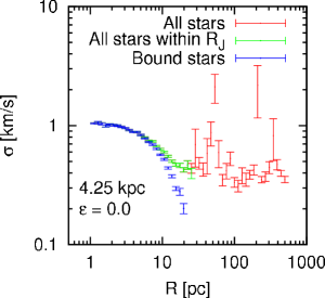
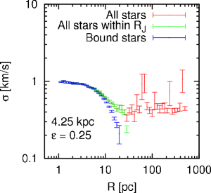
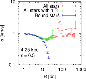
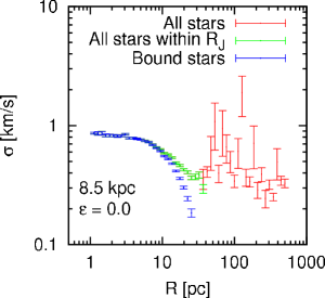
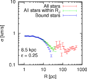
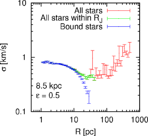
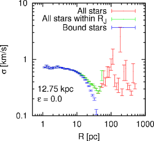
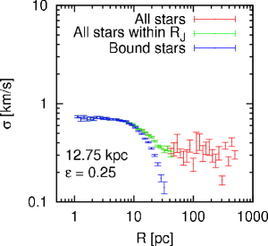
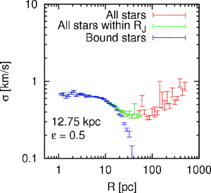
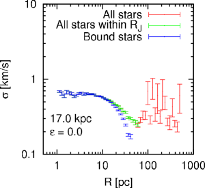
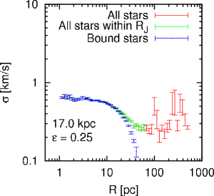
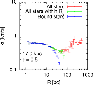
A typical sample of velocity dispersion profiles is shown in Fig. 2. In each graph the velocity dispersion is plotted i) for all stars in the sample (red), ii) for all stars that lie within the Jacobi radius (green), and iii) for all bound stars (blue).

The first column shows the clusters in a constant tidal field, i.e. on circular orbits. Comparing the graphs for the different galactocentric distances shows that, as expected, the clusters at larger galactocentric distances are more extended. Since they all have the same mass of about $15\,000\mbox{$\,{\rm M}_{\odot}$}$ in the snapshots, the central velocity dispersion decreases with $R_{G}$, whereas the size of the flat part within the core radius increases.

Each of the clusters in a constant tidal field has a steadily declining velocity dispersion within the Jacobi radius (green/red), although the clusters in the stronger tidal fields already show an onset of a flattening of the profile at the Jacobi radius. Beyond the Jacobi radius the velocity dispersion fluctuates strongly as the number statistics in these outer bins is quite low and a single fast escaper may dominate the velocity dispersion in the corresponding bin (red).

From the differently coloured curves we can see that the stars which lie within the projected Jacobi radius, but actually are in the foreground or background of the cluster within its tidal debris, hardly influence the velocity dispersion of the clusters (green). Only in some of the graphs can one make out a small contribution in the very outermost bins; everywhere else the green data points lie on top of the red ones.

By contrast, potential escapers have a significant influence on the profiles (green data vs. blue data). By definition the velocity dispersion of the bound stars approaches zero at the Jacobi radius, where the tidal forces are equal to the gravitational acceleration of the cluster. But we see a significant influence already at about 50% of the Jacobi radius.

4.1.2 Time-dependent tidal fields

Figure 3: Velocity dispersion profiles for the cluster D3, which is on an eccentric orbit with eccentricity 0.75 and an apogalactic distance of 17 kpc. The snapshots show the evolution of the profile with time during one revolution about the galactic centre, from apogalacticon to apogalacticon. In each graph the corresponding simulation time and galactocentric radius are given. In the middle graph the cluster is at perigalacticon. Here the Jacobi radius is at its minimum ($\sim$10 pc) and most of the cluster is unbound. For a large fraction of the orbit the velocity dispersion profile is approximately flat. Corresponding surface density profiles are given in Fig. 11.

If we take a look at columns 2 and 3 of Fig. 2 we can see the effect of time-dependent tidal fields on the velocity dispersion profiles. With increasing eccentricity the extent and onset of the population of potential escapers stays the same ($\sim 0.5R_{J}$), since in the snapshots all clusters are at apogalacticon. But from the green curve we can see that the energy of the potential escapers increases, which leads to a flattening of the velocity dispersion profiles. This is in agreement with findings by Gnedin, Lee & Ostriker (1999) who showed that stars at large radii are most affected by tidal perturbations like disk shocks or pericentre passages and that stars, on average, gain energy through such events. Furthermore, it supports the assumption of Küpper et al. (2010) that stars do not escape from the cluster immediately after a tidal perturbation, but can remain in the cluster for several cluster orbits about the galactic centre.

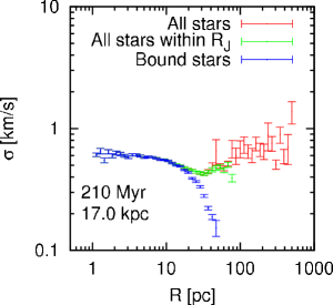
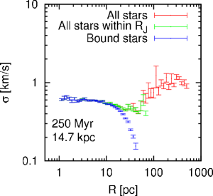
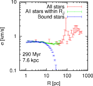
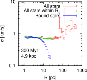
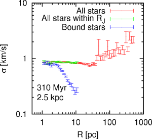
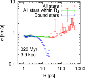
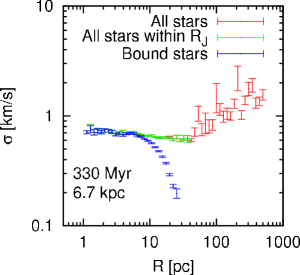
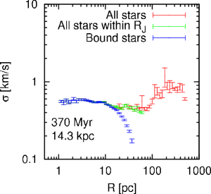
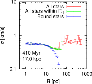
In Fig. 3 we show a time series of a cluster on an orbit with an eccentricity of 0.75 and an apogalactic radius of 17 kpc. The time series starts 210 Myr after the beginning of the computations, where the cluster is just about to finish its first revolution about the galactic centre and has a mass of $16\,200\mbox{$\,{\rm M}_{\odot}$}$. At 310 Myr (middle panel) the cluster is at perigalacticon with a mass inside the Jacobi radius of $7\,700\mbox{$\,{\rm M}_{\odot}$}$, and at 410 Myr it is again at apogalacticon with $13\,500\mbox{$\,{\rm M}_{\odot}$}$ left.

We see that for the largest part of the orbit, from 250 Myr to 370 Myr ($R_{G}<15$ kpc) the velocity dispersion profile appears to be more or less flat. For the perigalactic part of the orbit (300 Myr - 320 Myr, $R_{G}<5$ kpc) a good fraction of the cluster stars even lies beyond the Jacobi radius (about 50% of the apogalactic cluster mass). Nevertheless, even after such a dramatic pericentre passage the cluster’s velocity dispersion profile returns to nearly its original shape.

4.1.3 Concentrated clusters

Figure 4: Velocity dispersion profile for the concentrated cluster with a galactocentric radius of 4.25 kpc (A0c). At the time of the snapshot the cluster has a mass of about $15\,000\mbox{$\,{\rm M}_{\odot}$}$ and a ratio of projected half-mass radius to Jacobi radius of 0.08. Compared to the other clusters at the same stage of evolution, the velocity dispersion rises steeply in the centre due to core collapse, but shows a similar behaviour in the outer parts. A corresponding surface density profile is given in Fig. 13.

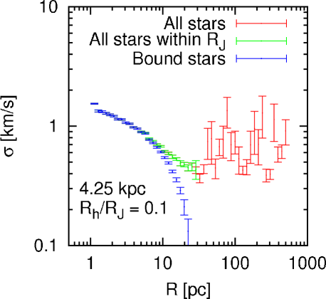
In Fig. 4 the velocity dispersion profile for a cluster at 4.25 kpc is shown. It had an initial (3-dimensional) half-mass radius of 3 pc, and is thus what Baumgardt et al. (2010) would classify as a compact cluster. At the time of the snapshot the cluster has $15\,000\mbox{$\,{\rm M}_{\odot}$}$ and still has a ratio of projected half-mass radius to Jacobi radius $R_{hp}/R_{J}=0.08$. The profile does not show a well-defined core in the range of the data points, as all other profiles do, but rises steeply in the centre. This is a clear indication of the fact that the cluster is near core collapse. Even so, there is no significant difference to the other clusters with respect to the potential escapers.

4.1.4 Conclusions

From the velocity dispersion profiles studied in this section we can conclude that the population of potential escapers has a significant influence on the kinematical structure of a star cluster. The influence of this population on the velocity dispersion profiles grows with increasing eccentricity of the cluster orbit. In such cases an observer would have to be very cautious when deriving a dynamical mass out of velocity dispersion measurements as it would tend to be overestimated, the possible degree of overestimation depending on the cluster characteristics such as its orbit and its velocity dispersion.

Furthermore, we saw that the velocity dispersion profile deviates from the expected Keplerian profile at a radius of about half the Jacobi radius. Since most globular clusters in the Milky Way experience a gravitational acceleration which is about the size of $GM_{Gal}/R_{Gal}^{2}\simeq 1.2\times 10^{-8}\mbox{cm s}^{-2}\simeq a_{0}$ one may easily be misled to deduced deviations from Newtonian gravity (e.g. Scarpa et al. 2007). To reduce the influence of potential escapers, velocity dispersion measurements should be made within 50% of the Jacobi radius. Nevertheless, extra caution has to be taken for clusters on eccentric orbits.

Moreover, we can see the general structure of star clusters already in the velocity dispersion profiles. There is a core which can be flat or cuspy. Then there is a bulk of bound stars whose limiting radius is somewhat smaller than the Jacobi radius, and finally there is the tidal debris whose onset lies within the Jacobi radius as a consequence of potential escapers. Most of this cluster structure is temporarily erased during pericentre passages for eccentric cluster orbits. By contrast, the concentrated clusters show a different cluster structure, as they do not seem to show a distinct core and bulk within the range of the data points.

4.2 Surface density profiles

4.2.1 Constant tidal fields

Figure 5: Surface density profiles of the cluster in a constant tidal field at a galactocentric distance of 8.5 kpc (B0). The upper panels of the first five graphs show the data and the template fits according to Sec. 3.4 for the five ranges of 1-[25, 50, 100, 200, 500] pc. The lower panels of the first five graphs give the relative deviation of the templates from the data. Vertical dashed lines mark the fitting range. The theoretical Jacobi radius can be read off from the outermost green data point (bound stars). The lower right panel shows the reduced $\chi^{2}$ for all of the five ranges, averaged over all snapshots of this cluster. Error bars give the standard deviation of $\chi^{2}_{red}$. A corresponding velocity dispersion profile is given in Fig. 2.

Figure 6: Evolution of the slopes of the tidal debris of the templates which can fit such a component, i.e. the surface density in the tidal debris falls off with $R^{-X}$, for the cluster on a circular orbit at 8.5 kpc (B0). Since the gen. Nuker template has two power-law slopes we show both here. Note that the Nuker and the gen. Nuker slopes are smoothed, as the variations between the individual time steps are very large. The other slopes are not smoothed since they are better behaved. The EFF and KKBH slopes show a rise in the beginning of the simulation which corresponds to an initial increased mass-loss rate due to primordial escapers. The Nuker and gen. Nuker slopes give no reliable information on the tidal debris slope.

Figure 7: Evolution of the Jacobi radius $R_{J}$ of the cluster on a circular orbit at 8.5 kpc (B0), evaluated using eq. 10 (red dotted line), and the edge radii of the fitted templates for a fit range of 1-100 pc. None of the edge radii reproduces the Jacobi radius well over the whole simulation time. King shows considerable evolution with respect to the Jacobi radius. The edge radius of the gen. Nuker template is smoothed since it fluctuates a lot, or sometimes does not converge properly (see text). In cases when it converges, it mostly gives a radius which is about 50% larger than $R_{J}$. KKBH has about the same values as King, though reduced by another 10%, but is less influenced by the initial mass loss due to primordial escapers, i.e. is more stable.

Figure 8: Ratio of the fitted edge radii to the Jacobi radius averaged over the whole simulation of the cluster on a circular orbit at 8.5 kpc (B0) and shown for all 5 fit ranges. Error bars give the standard deviations from the mean. The King template reproduces the Jacobi radius to about 10% accuracy for sufficiently large fit ranges. Gen. Nuker gives values 2-3 times larger than the Jacobi radius and shows large fluctuations. KKBH shows a constant value over all fit ranges which is about 20% smaller than the Jacobi radius. Also shown are the edge radius of the bound stars, which lies at about 70% of $R_{J}$, and the break radius of the KKBH template at which the profile of the cluster becomes dominated by potential escapers.

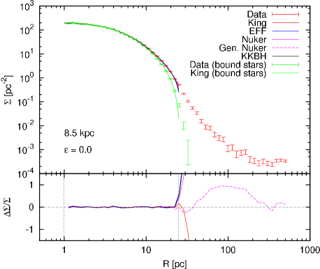
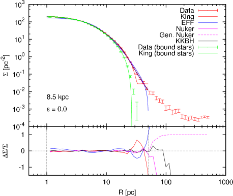
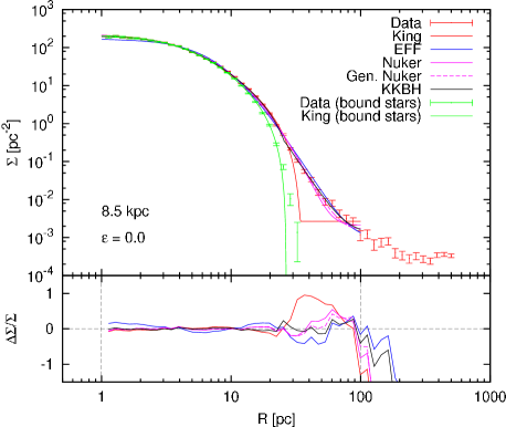
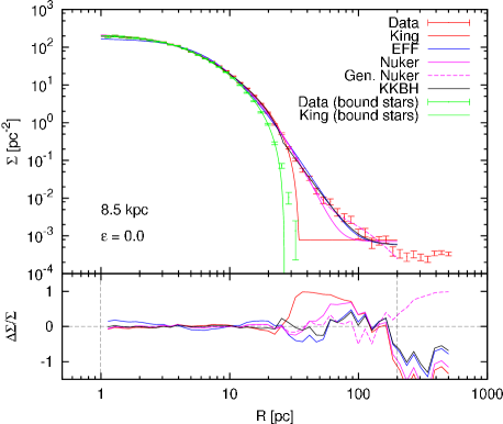
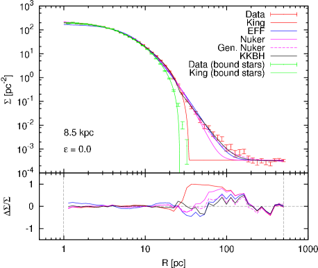
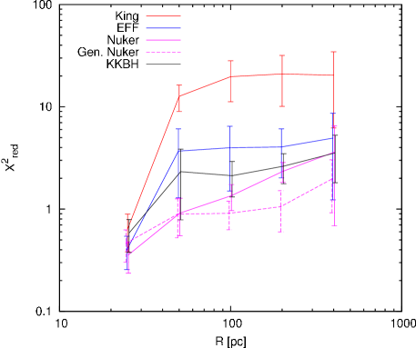
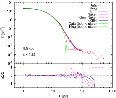
As an example to demonstrate the fitting process, in Fig. 5 the surface density profile of the cluster on a circular orbit at 8.5 kpc is shown when the cluster has a mass of $15\,000\mbox{$\,{\rm M}_{\odot}$}$, just as was shown for the velocity dispersion in the 4th panel of Fig. 2. In the upper panels of the first five graphs the cluster data and the fits of the analytical templates from Sec. 3.4 are shown for the five different ranges of 1-[25, 50, 100, 200, 500] pc. In the lower panels of these graphs the relative errors can be seen. The lower right panel gives the reduced $\chi^{2}$ for each template for each fit range averaged over all 400 snapshots of the cluster.

We see that for the smallest fit range (1-25 pc) all templates fit about equally well, whereas for the larger ranges significant differences in the quality of the fits appear. This is due to the fact that the smallest fit range only covers the core of the cluster, which in this case is flat, and a part of the bulk. Such a profile can be fit by all templates in the sample. But already the second smallest fit range of 1-50 pc covers part of the tidal debris, as the Jacobi radius in this snapshot is 36 pc. Hence the King template, which does not have a proper tidal debris term, gets significantly worse with increasing fit range. Furthermore, since there is an inflexion point of the slope between the bulk and the tidal debris at about the Jacobi radius, the templates which cannot account for the bulk and debris separately (EFF and Nuker) get worse for increasing fit range as well. In contrast to EFF, however, Nuker can partially compensate the missing bulk term by a more flexible core term. Besides Nuker, only the two templates which consist of three parts have a good reduced $\chi^{2}$ value over all fit ranges (lower right panel of Fig. 5).

Taking a closer look at the tidal debris of this cluster at the given, dynamically well-evolved state shows that the slope outside the Jacobi radius is quite similar to the slope of the bulk, though it is not the same. If the data had been slightly more noisy we could have even concluded that the slope of the tidal debris close to the cluster is the same as the slope of the bulk, which is what Elson, Fall & Freeman (1987) might have seen in their data on young LMC clusters. This is also the reason why EFF and Nuker fit this cluster reasonably well even though they have no separate bulk and debris terms.

Another striking fact is that the tidal debris does not show a constant slope for radii much larger than the Jacobi radius. From a constant mass-loss rate (which this cluster shows for several Gyr) and a constant velocity of the escapers within the tidal tails away from the cluster we would infer that the number of stars in the debris grows linearly with radial distance from the cluster. Thus, the surface density profile of the debris should fall off with $R^{-1}$, as the surface area of the annuli grows with $R^{2}$. Instead we see a slope which is steeper close to the cluster and gets more shallow at radii of several hundred pc.

This is due to the fact that stars do not move linearly along the tidal tails as they escape from the cluster, but exhibit an epicyclic motion in which they get periodically accelerated and decelerated (Küpper, Macleod & Heggie, 2008). Since escaping stars are first accelerated away from the cluster, the slope of the surface density close to the cluster should be lower than -1. This acceleration then turns into a deceleration at a distance $R=0.5\,y_{C}$, where the length of the epicycles, $y_{C}$, depends on the tidal field. At a distance $R=y_{C}$, which in this case is given by approximately $3\pi R_{J}\simeq 340$ pc, the slowest escapers (escapers with $E-E_{crit}\simeq 0$) are coming to a halt before they get re-accelerated. Escapers with a finite velocity above the escape velocity come to a halt at a somewhat larger $y_{C}$, so that the mean escaper reaches its lowest drift velocity along the tidal tails at about 400-500 pc. (For a detailed description of the tidal tails of this particular cluster see Küpper et al. 2010). In this range the slope of the surface density profile should be significantly larger than -1.

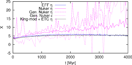
Of greatest interest with regard to real star clusters is the tidal debris close to the clusters, as observations barely extend to radii of several Jacobi radii. Thus, we focus on the inner 100 pc in the following discussion. In Fig. 6 the evolution of the power-law slopes of the tidal debris can be seen as fitted by the given templates for a fit range of 1-100 pc. We see that EFF and KKBH have a similar evolution, though KKBH varies less with time. This is due to the fact that EFF fits one slope for the bulk of the cluster and the tidal debris, whereas KKBH decouples the two parts and therefore gives a more accurate value for the slope of the tidal debris close to the cluster. As expected, the slope is significantly smaller than -1; indeed it has a value of about -5. Note that KKBH and EFF show a slightly shallower slope at the beginning of the simulation, where the cluster loses more mass as a consequence of primordial escapers (see Küpper et al. 2010). By contrast, we see that the Nuker and the gen. Nuker templates do not give reliable information on the tidal debris slope. The power-law slopes of the Nuker and the gen. Nuker templates in Fig. 6 even had to be smoothed in order to reduce the stochastic noise to a reasonable level. Even so, the fluctuations in the values are too large to allow any conclusions to be drawn from them. This is due to the factors $\alpha$ and $\delta$ in eq. 19 & 20 which are meant to adjust the smoothness of the transition from one slope to another but have quite a large influence on the fitting results.

From Fig. 5 we can see that the surface density of bound stars falls off more steeply than the surface density of all stars in the sample (green profile vs. red profile), i.e. the edge of the bulk of bound stars lies further in than the edge of the bulk of all stars. Thus, the population of potential escapers enhances or even dominates the surface density profile for radii larger than about half the Jacobi radius, just as we saw in the velocity dispersion profiles (Fig. 2). It should be kept in mind, however, that the underlying investigation is limited to star clusters with up to 64k stars. How this behaviour changes with increasing $N$ still has to be considered. From Baumgardt (2001), however, we expect only a weak dependence on $N$.

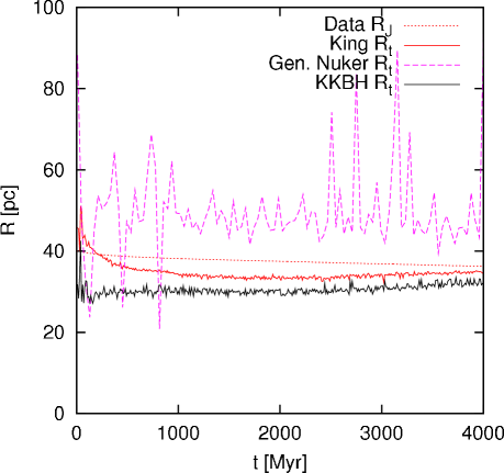
In Fig. 7 the time evolution of the Jacobi radius of this cluster is shown. As the cluster constantly loses mass the Jacobi radius (eq. 10) slowly decreases. Also shown in the figure are the fitted edge radii of the King, the gen. Nuker and the KKBH templates for a fit range of 1-100 pc. We see that none of the templates reproduces the Jacobi radius accurately over the whole simulation time.

The King $R_{t}$ shows strong evolution at the beginning, because of an initial burst of mass-loss due to primordial escapers, which the template tries to fit. For the rest of the simulation the King edge radius agrees with the Jacobi radius to within about 10%.

The gen. Nuker $R_{t}$ shows large fluctuations, which are due to the above mentioned smoothness parameters $\alpha$ and $\delta$, which introduce a large ambiguity but also cause problems in the fitting process. Thus, for this template the Marquardt-Levenberg algorithm sometimes does not converge properly, and then the starting value for $R_{t}$, which was chosen to be 90 pc for all templates, is retained. In case the fit converges, it mostly yields an edge radius which is about 50% too large.

The KKBH template usually yields similar results to King, though 10% smaller, but is much less influenced by the initial mass loss of primordial escapers, and thus more accurately reproduces the edge radius of the bulk of the cluster. This case is a good example in which heavy mass loss significantly influences fitting results, as may have happened in the investigation of Elson, Fall & Freeman (1987), or as was mentioned by Côté et al. (2002), Carraro, Zinn & Moni Bidin (2007) and Carraro (2009) for the Milky-Way globular clusters Palomar 13, Whiting 1 and AM 4, respectively. The structure of the KKBH template helps to minimise such a problem.

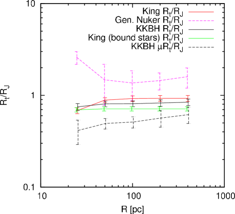
In Fig. 8 we show all these fitted edge radii in units of the Jacobi radius, averaged over all time steps of the simulation, for all 5 fit ranges. King shows a value which lies within 10% of the true Jacobi radius for large fit ranges. Only the smallest fit range of 1-25 pc yields an average edge radius which is about 30% off, so here the fit range would significantly influence the fitting result. In contrast to that the KKBH template gives a more constant value over all fit ranges but which is reduced compared to King by about 10%. The gen. Nuker template does not yield a reliable value for the edge radius, as the fluctuations between the time steps are large, as indicated by the error bars, and the mean strongly depends on the fit range.

Throughout the analysis we found the bound stars to be well represented by a simple King template. From Fig. 8 we see that the edge of bound stars lies at about 70% of the Jacobi radius. The break radius of the KKBH template, at which it changes into the power-law tidal debris, is also shown in the figure and lies at about 50% of $R_{J}$ and can be interpreted as the radius at which the profile of the cluster deviates from a smooth bulk profile and gets dominated by potential escapers.

In Tab. 3 a summary of the fitting results of the edge radii for the three smallest fitting ranges for all clusters in a constant tidal field is given. From this table we can conclude that the edge radii are closer to the Jacobi radius the larger the fit range is. For the smallest fit range the deviation can be even up to 40%. Averaging over all the fitting results in Tab. 3 confirms our findings: the King edge radius is on average a little (10-20%) smaller than the true Jacobi radius. Gen. Nuker yields no reliable results, whereas KKBH is more stable than King but yields an edge radius which is also about 20% smaller than the true Jacobi radius. Furthermore we see from the table that the edge of bound stars lies at about 70% of the Jacobi radius and that KKBH finds a break in the profile slope at about 50% of the Jacobi radius. Thus, at this radius the profile becomes dominated by potential escapers.

From the investigation of the clusters in a constant tidal field we can conclude that our ansatz for constructing a star cluster template consisting of core, bulk and debris was chosen well. The unbound tidal debris has a significant influence on the fitting results, but this can be minimised by the addition of an independent tidal debris term. In addition, our constructed KKBH template is a good tool with which to measure the power-law slope of the tidal debris and to look for a break in the surface density profile. In this way we saw that the influence of potential escapers on the cluster profile is significant for radii larger than 0.5$R_{J}$ and that beyond about 0.7$R_{J}$ nearly all stars are unbound.

4.2.2 Time-dependent tidal fields

Figure 9: Surface density profiles of the clusters at an apogalactic distance of 8.5 kpc with an orbital eccentricity of 0.25 (B1, left) and 0.5 (B2, right). At the time of the snapshot both clusters are at apogalacticon and have a mass of about $15\,000\mbox{$\,{\rm M}_{\odot}$}$. The power-law slope of the tidal debris as measured by the KKBH template is $\eta=5.2\pm 0.3$ on the left and $\eta=4.5\pm 0.2$ on the right. The inner cluster profiles look quite similar whereas the average density outside the cluster with an orbital eccentricity of 0.5 is higher, which is due to the higher mass-loss rate of this cluster and the larger orbital compression of its tidal tails. The theoretical Jacobi radii can be read off from the outermost green data points (bound stars). Corresponding velocity dispersion profiles are given in Fig. 2.

Figure 10: Evolution of the slopes of the tidal debris of the templates as shown in Fig. 6 for the clusters with an apogalactic distance of 8.5 kpc and an orbital eccentricity of 0.25 (B1, upper panel) and 0.5 (B2, lower panel). The Nuker and the gen. Nuker slopes are smoothed with a cubic spline, as the variations between the individual time steps are very large. The EFF and KKBH (for $\epsilon=0.5$ also the Nuker) slopes again show a similar evolution around an average value of about $\eta=5$. For increasing orbital eccentricity the power-law slope of the tidal debris starts to vary with the orbital phase. As the cluster gets compressed close to apogalacticon, the slope of the tidal debris abruptly decreases to values of about $\eta=2-3$.

Figure 11: Surface density profiles for the cluster at an apogalactic distance of 17 kpc with an orbital eccentricity of 0.75 (D3). On the left the cluster is shown shortly before reaching apogalacticon, in the middle it is at apogalacticon whereas on the right it is at perigalacticon. The power-law slope of the tidal debris as measured by the KKBH template is $\eta=1.7\pm 0.2$ on the left, $\eta=2.9\pm 0.5$ in the middle and $\eta=3.8\pm 0.1$ on the right. Close to and at apogalacticon the cluster and its tidal tails get heavily compressed which leads to a great enhancement in the number of stars close to the cluster. At perigalacticon most of the profile is best fit by a power-law. Furthermore, most stars are unbound (green line), just as we have seen in the velocity dispersion profile (middle graph of Fig. 3). The drop in surface density in the left and middle panel for large radii is due to the young age of the cluster and its short tails, as escaped stars simply could not travel far at this time. Corresponding velocity dispersion profiles are given in Fig. 3.

Figure 12: Evolution of the Jacobi radii, evaluated using eq. 10 (red dotted line), and the edge radii of the fitted templates for a fit range of 1-100 pc for the clusters with an apogalactic distance of 8.5 kpc and an orbital eccentricity of 0.25 (B1, upper panel) and 0.5 (B2, lower panel). The line colours are the same as in Fig. 7. Even though the Jacobi radius changes periodically the bulk of the cluster seems to be unaffected. The evolution of the King and KKBH edge radii (red and black solid line) are very much like in Fig. 7 but shifted to lower values for increasing orbital eccentricity. Only the break radius of the KKBH template (black dashed line) seems to be somewhat affected by the changing tidal field.

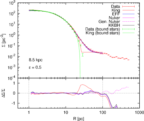
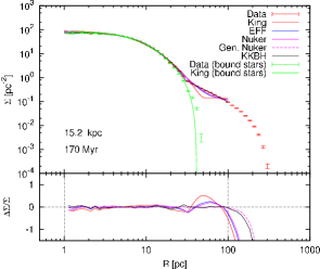
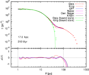
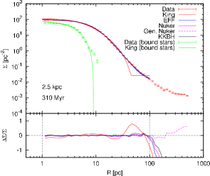
In Fig. 9 we see the clusters with an orbital eccentricity of 0.25 (left panel) and 0.5 (right panel) at the time when they are at their apogalactic distance of 8.5 kpc, just as shown in Fig. 2 for the velocity dispersion profiles. Also shown in the figure are the template fits for a fit range of 1-100 pc. We see no significant difference from the surface density profile of the cluster on a circular orbit (Fig. 5), except for the mean density within the tidal debris, which gets larger with increasing eccentricity. This is due to the average mass loss of the clusters as well as the orbital compression of the tails at apogalacticon, which both increase with eccentricity.

The slope of the tidal debris close to the cluster ($\sim R^{-\eta}$) is $\eta=5.2\pm 0.3$ for $\epsilon=0.25$ and $\eta=4.5\pm 0.2$ for $\epsilon=0.5$, i.e. about the same as in the constant tidal field (about $\eta=5$ for $\epsilon=0.0$). But since the cluster has a lower orbital velocity at apogalacticon for increasing eccentricity, the epicyclic overdensities in the tidal tails are also located closer to the cluster (see Küpper et al. 2010) and the surface density is enhanced relative to the circular case.

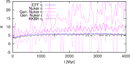
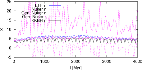
From Fig. 10 we see that for a small orbital eccentricity of $\epsilon=0.25$ the tidal debris slope evolves very much as in the constant tidal field case. For $\epsilon=0.5$ we see that the slope on average shows the same evolution, but in addition shows jumps to smaller values. These jumps occur shortly before apogalacticon where the tails get maximally compressed due to the orbital acceleration, so that, for large eccentricities, they literally get pushed back inside the cluster. This enhances the tidal debris close to the cluster and thus temporarily yields a shallower slope. This effect is shown in Fig. 11 for the cluster with an apogalactic distance of 17 kpc and an orbital eccentricity of 0.75. The left panel shows the cluster close to apogalacticon, the middle panel shows it at apogalacticon whereas the right panel shows the cluster at perigalacticon, similar to what we have seen in Fig. 3. The slopes $\eta$ of the three snapshots as measured by the KKBH template are $\eta=1.7\pm 0.2$ close to apogalacticon, $\eta=2.9\pm 0.5$ at apogalacticon and $\eta=3.8\pm 0.1$ at perigalacticon.

Summarising the results, including also those from all the other models of our systematic study, which are not shown here in detail, we can conclude that the tidal debris close to the cluster (up to about three times the Jacobi radius) has a power-law slope $\eta$ in the range 4 to 5, which can decrease to values in the range 1-2 shortly before apogalacticon due to orbital compression of the tidal tails. This may lead to the conclusion that we can identify those star clusters which are at an orbital phase close to apogalacticon by the slope of their surface density profiles outside the Jacobi radius. Star clusters like Palomar 13, AM 4 and Whiting 1 may well be in such an orbital phase, as their surface density profiles show slopes of about $\eta=1.8$ (Côté et al., 2002; Carraro, Zinn & Moni Bidin, 2007; Carraro, 2009). This assumption is further strengthened by the Milky-Way globular cluster Palomar 5, whose orbit is well constrained due to its long tidal tails (Dehnen et al., 2004). It is currently located close to apogalacticon and shows a power-law slope of about -1.5 (Odenkirchen et al., 2003).

From the right panel of Fig. 11 we can see that at perigalacticon, where the Jacobi radius is smallest (about 10 pc), most of the cluster is unbound (green data points vs. red data points) just as we have seen in the corresponding velocity dispersion profile (middle panel of Fig. 3). Also note here how much more poorly the King template fits the cluster at perigalacticon than at apogalacticon. By contrast, the KKBH template, as well as the others with a power-law tidal debris term, can cover the whole cluster and its debris perfectly well.

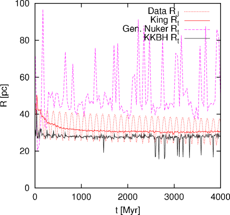
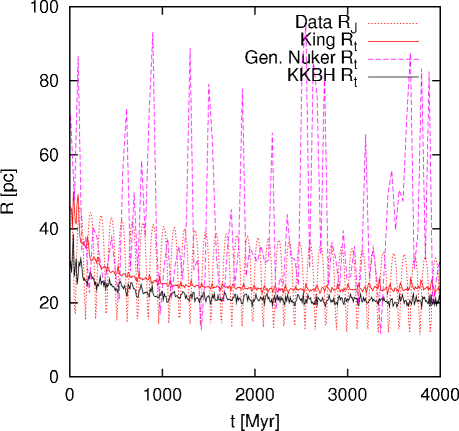
In Fig. 12 we show the evolution of the Jacobi radius and of the fitted edge radii for the above clusters with eccentricities of 0.25 and 0.5, just as in Fig. 7 for $\epsilon=0.0$. While the Jacobi radius oscillates with an amplitude which increases with increasing eccentricity, the overall evolution of the other radii is very similar to the constant tidal field case. The edge radius of the King template shows some evolution at the beginning but then gives the mean Jacobi radius of the cluster. The KKBH template again shows less evolution than King at the beginning, i.e. is less affected by heavy initial mass loss, but again gives a nearly constant value similar to that of King, but reduced by about 10%. The gen. Nuker edge radius does not show a well-behaved evolution at all.

The results from all models on eccentric orbits in our set are presented in Tab. 4-6 sorted by eccentricity. The results of the clusters with $\epsilon=0.25$ and $\epsilon=0.5$ agree well with the findings for the clusters in a constant tidal field (Tab. 3). We note especially the consistent values for the edge of the bound stars at 70% of the Jacobi radius and the break radius of the KKBH template at 50% of the Jacobi radius. But also the fact that the King template yields on average about 90% of the mean Jacobi radius is interesting, since it is commonly thought that observed edge radii correspond to the perigalactic Jacobi radii of the corresponding clusters. The fact that the edge radius is not set at perigalacticon is due to the fact that stars do not leave the cluster immediately after becoming unbound but stay within the Jacobi radius for up to several orbits of the cluster about the galaxy. Moreover, when we consider the elongated shape of the equipotential surfaces of a cluster in a tidal field it is quite reasonable that a spherically symmetric, one-dimensional density profile will yield a smaller value than the two-dimensional (i.e. projected) Jacobi radius.

Note that the mean results and fluctuations get worse for increasing tidal field strength. All clusters with orbital eccentricities of 0.75 get disrupted within a few orbits about the galactic centre and thus are barely in a state close to virial equilibrium. Also the clusters at 4.25 kpc and 8.5 kpc with eccentricities of 0.5 show large spreads in the fits as they penetrate deeply into the central part of the galaxy. At the beginning of these $N$-body computations, however, when the clusters are still very massive and much less vulnerable to tidal influences, the fitting results are more stable and agree with the findings for the other clusters.

From the clusters in time-dependent tidal fields we can conclude that our KKBH template again proves to be a good tool to investigate the state of the clusters and their tidal debris. Thus, we were able to extend our findings of the previous section to clusters on eccentric orbits. Moreover, we suggest that star clusters in an orbital phase close to apogalacticon can be identified by the slope of their surface density profile outside the Jacobi radius. We furthermore find that the bulk of the cluster adjusts to the mean tidal field rather than, as usually believed, to the perigalactic tidal field.

4.2.3 Concentrated clusters

Figure 13: Surface density profiles of the concentrated clusters at a galactocentric radius of 4.25 kpc (A0c, left) and 12.75 kpc (C0c, right). At the time of the snapshots both clusters have a mass of about $15\,000\mbox{$\,{\rm M}_{\odot}$}$. The power-law slope of the tidal debris as measured by the KKBH template is $\eta=4.6\pm 0.6$ (left) and $\eta=4.3\pm 0.3$ (right). The theoretical Jacobi radii can be read off from the outermost green data points (bound stars). One corresponding velocity dispersion profile is given in Fig. 4.

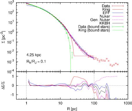
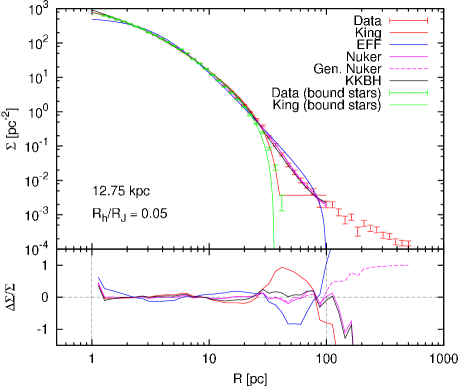
Fig. 13 shows the surface density profiles of the clusters at 4.25 kpc (left) and 12.75 kpc (right), which both had an initial (3-dimensional) half-mass radius of 3 pc; for the first of these the corresponding velocity dispersion profile was shown in Fig. 4. At the time of the snapshots the clusters have $15\,000\mbox{$\,{\rm M}_{\odot}$}$ and a ratio of projected half-mass radius to Jacobi radius of 0.08 (left) and 0.06 (right). From the figures and the fitted templates we see that the power-law slope of the tidal debris agrees with the previous findings ($\eta=4.6\pm 0.6$ for the left panel and $\eta=4.3\pm 0.3$ for the right). Furthermore, we see that the EFF template completely fails to fit the data. This is due to the fact that the clusters do not have a distinct core (at least down to a radius of 1 pc) but appear to consist only of a bulk and tidal debris. Thus the EFF template, which consists of a flat core and a tidal debris term, cannot reproduce it. The King template does a better job for the bulk but fails at the edge of the bulk, whereas KKBH can give a good representation of all parts of both clusters. Nuker and gen. Nuker are also flexible enough to cover the whole radial range. These characteristics become more pronounced for increasing galactocentric radius as the half-mass radius is fixed at 3 pc but the Jacobi radius increases, and so the concentration increases. Note also that the quality of the King template fit decreases with a larger concentration. This supports the findings by Baumgardt et al. (2010) that concentrated clusters cannot be properly fitted by a King template.

But even though most templates yield good $\chi^{2}$ values, from Tab. 7 we can see that the fitted edge radii do not correspond to the Jacobi radii any more. With increasing concentration the edge radii shrink compared to the Jacobi radii. That is the reason why we avoid the term tidal radius and instead use edge radius, since this edge radius does not have to be a result of the galactic tide.

Moreover, since the bound stars follow a similarly concentrated distribution and since we tried fitting this distribution with a King template, these numbers also get unreliable. Here a reconsideration of the templates with regard to the structure of concentrated clusters would be necessary, since the templates we used here all seem to fail in giving information on the cluster structure, due to the fact that these clusters do not show a distinct core and bulk down to 1 pc. Thus, we conclude that Jacobi radii cannot be reliably determined from observed clusters using these templates if their concentration is high, i.e. with $R_{hp}/R_{J}\simeq 0.1$ or smaller.

4.3 Review of templates

Before summarising the results of this investigation let us briefly discuss the performance of the templates which were defined in Sec. 3.4 and which were used here.

• King has proved to be a reasonable tool for studying the Jacobi radius of extended clusters but fails when the cluster has a pronounced tidal debris component or is too concentrated. It cannot give information on the core slope of either mass segregated clusters or clusters with an IMBH in the centre. Eccentric cluster orbits are also a problem for the template. Moreover, the fit results strongly depend on the radial range of the cluster which is covered; it is thus quite unreliable for obtaining cluster parameters.

• EFF is a good tool for the study of clusters with a pronounced tidal debris component, provided that they are not too concentrated or mass segregated. It cannot, however, give information on the edge radius.

• Nuker can fit most of the clusters in our sample well, but it is not possible to deduce cluster parameters reliably from the fitting results. Furthermore it does not have an edge radius.

• Gen. Nuker is a very powerful template with a low $\chi^{2}$ for all fit ranges but, just as Nuker, does not allow the deduction of reliable structural parameters from the fitting results, as the resulting parameters of the template vary strongly and depend strongly on the radial coverage of the cluster.

• KKBH has proved to be a reasonable extension of King, improving the fitting results for all clusters in the sample. It also yields the most reliable structural information over all fit ranges in terms of edge radius and the slope of the tidal debris. Like all other templates, however, it fails in the case of concentrated clusters.

5 Conclusions

This systematic investigation of velocity dispersion profiles and surface density profiles of star clusters with masses of about $10^{4}\mbox{$\,{\rm M}_{\odot}$}$ has shown how complex and versatile these profiles can be, depending on the circumstances of the clusters.

Furthermore we have shown the importance of potential escapers for these two quantities. Both profiles are influenced by this population of energetically unbound stars for radii larger than about 50% of the Jacobi radius and are completely dominated by it for radii larger than about 70% of the Jacobi radius (Fig. 2 & 3). Baumgardt (2001) found that for clusters in a constant tidal field the fraction of potential escapers varies with the number of stars within a cluster approximately as $N^{-1/4}$. Thus, even if the cluster mass increases by a factor of 10, the fraction (and influence) of potential escapers will only be reduced by less than 50% compared to this investigation.

As a consequence of the potential escaper population, the velocity dispersion profiles in our sample do not show a clear separation between the bulk of the cluster and the tidal debris at the Jacobi radius, but rather show a smooth transition from cluster to debris. For mass estimates which are based on velocity dispersion measurements we therefore recommend to use stars within 50% of the Jacobi radius to minimise the effect of potential escapers.

Moreover, we argue that investigations on velocity dispersion profiles like Drukier et al. (1998), Scarpa, Marconi & Gilmozzi (2003) or (Scarpa et al., 2007) have to be interpreted with caution. Also, detecting a possible dark matter halo around globular clusters is less feasible due to the population of potential escapers. Based on our investigation we suggest that no deviation from Newtonian gravity in a star cluster has been detected so far, neither has there been evidence for a dark matter halo.

From our large set of surface density profiles we saw that in most cases the structure of extended star clusters can be split into core, bulk and tidal debris.

1. The core is the innermost part of the cluster which extends out to the core radius. In most cases it is flat, and only for clusters with strong mass segregation or with an IMBH is it cuspy. Very concentrated clusters with $R_{hp}/R_{J}<0.1$ have such a small core that fitting such clusters leads to problems with templates as well as with physical models (see also Baumgardt et al. 2010).
   
   

2. The bulk contains most stars of the cluster and extends from the core to the tidal debris. We found that the bulk can be well represented by a King-like template. We named the radius at which such a template approaches zero density the edge of the bulk and not the tidal radius of the cluster, since we found it not to be consistent with the Jacobi radius. In the case of concentrated clusters, the edge radius is not even determined by tidal forces at all (Tab. 7).
   

   Moreover, for clusters on eccentric orbits we found that the edge radius of a cluster adjusts to the mean Jacobi radius (Fig. 12) and not the perigalactic Jacobi radius, which has been assumed in earlier investigations (e.g. Innanen, Harris, & Webbink 1983, Fall & Zhang 2001), but has never been checked by self-consistent calculations on a star-by-star basis. Since nearly all globular clusters of the Milky Way are more compact and massive than our test cluster, and thus should be less influenced by tidal variations, this finding should also hold for most of these clusters.
   

   The edge radius of extended and moderately concentrated clusters, as fitted by the King template, lies within about 10% accuracy at  90% of the mean Jacobi radius (Tab. 3-6). But we found the King template to be a bad representation of the true profile in the case of non-circular cluster orbits because it is significantly influenced by the tidal debris and by the potential escaper population. Furthermore the accuracy of the results strongly depends on the radial coverage of the cluster. We therefore created an enhanced version of the King template which has more flexibility in the core and has an additional tidal debris term, given by a power-law. With this KKBH template we achieved a higher stability over all fit ranges. Furthermore, we were able to measure the edge of the bulk more accurately and found it to lie at 80% of the Jacobi radius. This discrepancy is easily understandable if we take into account the fact that the edge radius of a template fits the azimuthally averaged mean of a cluster’s tidal surface, whereas the Jacobi radius is by definition the semi-major axis of the equipotential surface.
   

   Furthermore we found that the edge radii from concentrated clusters with $R_{hp}/R_{J}<0.1$ cannot be extracted properly with currently available templates. The higher the concentration of the cluster the smaller is the ratio of the fitted edge radius to the theoretically evaluated Jacobi radius (Tab. 7).
   
   

3. The tidal debris falls off like a power-law with a slope of about -4 to -5, rather than the expected dependence of $R^{-1}$. This is due to the epicyclic motion of the stars in the tidal tails, which is most pronounced in the vicinity of the cluster.
   

   For clusters on eccentric orbits, at a time shortly before reaching apogalacticon, the slope was found to deviate for a short time to a value of about -2 as a consequence of orbital compression of the tails (Fig. 10 & 11). We suggest that this enhanced slope can be used to identify star clusters which are close to or at the apogalacticon of their orbit. The most prominent example of such a cluster is the Milky Way globular cluster Palomar 5 which is well known to be close to the apogalacticon of its orbit (Dehnen et al., 2004), and which shows a power-law slope of -1.5 outside its assumed Jacobi radius (Odenkirchen et al., 2003). Moreover, the MW globular clusters Palomar 13, AM 4 and Whiting 1 may be further candidates for being close to apogalacticon, since their surface density profiles show power-law slopes of about -1.8 outside the Jacobi radius, which has been attributed to heavy ongoing mass loss by the authors of the corresponding investigations (Côté et al., 2002; Carraro, Zinn & Moni Bidin, 2007; Carraro, 2009).
   

   Furthermore we showed that due to the population of potential escapers the power-law slope of the tidal debris begins even before the Jacobi radius is reached. Thus, the bulk and the tidal debris partially overlap. With our KKBH template we found the debris to dominate for radii larger than about 50% of the Jacobi radius (Tab. 3-6).

With the help of our comprehensive set of clusters it is possible to tailor a star cluster template to the facts we have found. Our KKBH template seems to be a good first step but, like all other available templates, shows discrepancies for concentrated clusters. Of course, templates are less attractive than physically motivated models. None of the existing models, like King (1966) and Wilson (1975), however, account for the above mentioned facts. We suggest that a general, physically motivated model for star clusters should include a term for mass segregation and should include a potential escaper population when being fitted to observations. Finally, the possible influence of (compressed) tidal tails on the surface density profiles of star clusters should be kept in mind when fitting surface density profiles.

Moreover, the fact that all clusters in the sample showed a constant edge of the bulk with time (Fig. 12) and that stars which get unbound escape from a cluster with a delay, supports our theoretical treatment of epicyclic overdensities in tidal tails for clusters in time-dependent tidal fields in Küpper et al. (2010).

Appendix A Fitting KKBH using GNUPLOT

When using gnuplot, fitting the KKBH template is quite simple since it is possible to use ternary operators. First the two functions $f_{1}(R)$ and $f_{2}(R)$ (eq. 22 & 23) need to be defined with

f1(x) = (x<Rt ? k * (x/Rc/(1.0+x/Rc))**(-gamma) * (1.0/(1.0+(x/Rc)**2.0)**(0.5) - 1.0/(1.0+(Rt/Rc)**2.0)**(0.5))**2.0 : 0)

and

f2(x) = f1(Rt*mu) * (1.0 + (x/(Rt*mu))**64.0)**(-eta/64.0)

after which the KKBH function is defined

f(x) = (x < mu*Rt ? f1(x) + b : f2(x) + b)

is defined. Then the constants have to be set to some reasonable value, e.g.

k = 1.0
Rc = 5.0
gamma = 0.01
Rt = 50.0
mu = 0.5
eta = 3.0
b = 0.0001

If surface density data exists in a file named, e.g., data.txt, with columns $R$, $\Sigma(R)$ and $\Delta\Sigma(R)$, the final fitting is carried out by use of the command

fit f(x) $\prime$data.txt$\prime$ u 1:2:3 via k, Rc, gamma, Rt, eta, mu, b.

Appendix B Data tables

Table 3: Fitting results for the edge radii in units of the theoretical Jacobi radius for the clusters in a constant tidal field averaged over all available snapshots of the specific model. The results are given for the three smallest fit ranges. In the last line a weighted mean and the standard deviation of the results is given. $R_{t}$ gives the edge radius of the specific template, whereas $R_{J}$ stands for the theoretical Jacobi radius. $\mu$ is the fraction of the edge radius, at which the KKBH template turns into a power-law.

Name	fit range	King	Gen. Nuker	KKBH		King (bound)
	$[\mbox{pc}]$	$\frac{R_{t}}{R_{J}}$	$\frac{R_{t}}{R_{J}}$	$\frac{\mu R_{t}}{R_{J}}$	$\frac{R_{t}}{R_{J}}$	$\frac{R_{t}}{R_{J}}$
A0	1-25	0.86 $\pm$ 0.06	3.70 $\pm$ 0.86	0.49 $\pm$ 0.09	0.82 $\pm$ 0.07	0.77 $\pm$ 0.47
	1-50	0.97 $\pm$ 0.06	2.12 $\pm$ 0.98	0.53 $\pm$ 0.08	0.85 $\pm$ 0.07	0.74 $\pm$ 0.13
	1-100	0.98 $\pm$ 0.06	2.22 $\pm$ 0.97	0.57 $\pm$ 0.11	0.86 $\pm$ 0.08	0.74 $\pm$ 0.13
B0	1-25	0.68 $\pm$ 0.05	2.58 $\pm$ 0.41	0.41 $\pm$ 0.12	0.75 $\pm$ 0.06	0.70 $\pm$ 0.04
	1-50	0.89 $\pm$ 0.05	1.48 $\pm$ 0.70	0.49 $\pm$ 0.06	0.81 $\pm$ 0.06	0.71 $\pm$ 0.04
	1-100	0.92 $\pm$ 0.07	1.36 $\pm$ 0.49	0.51 $\pm$ 0.07	0.81 $\pm$ 0.06	0.71 $\pm$ 0.04
C0	1-25	0.63 $\pm$ 0.04	1.94 $\pm$ 0.35	0.60 $\pm$ 0.05	0.76 $\pm$ 0.03	0.67 $\pm$ 0.02
	1-50	0.84 $\pm$ 0.01	1.56 $\pm$ 0.89	0.46 $\pm$ 0.05	0.79 $\pm$ 0.03	0.71 $\pm$ 0.01
	1-100	0.92 $\pm$ 0.05	1.36 $\pm$ 0.74	0.50 $\pm$ 0.05	0.81 $\pm$ 0.03	0.71 $\pm$ 0.01
D0	1-25	0.56 $\pm$ 0.05	1.58 $\pm$ 0.26	0.57 $\pm$ 0.02	0.71 $\pm$ 0.02	0.63 $\pm$ 0.01
	1-50	0.78 $\pm$ 0.01	1.32 $\pm$ 0.96	0.39 $\pm$ 0.03	0.76 $\pm$ 0.02	0.71 $\pm$ 0.01
	1-100	0.90 $\pm$ 0.05	1.20 $\pm$ 0.74	0.49 $\pm$ 0.05	0.80 $\pm$ 0.03	0.71 $\pm$ 0.03
mean		0.81 $\pm$ 0.14	1.84 $\pm$ 0.72	0.50 $\pm$ 0.06	0.78 $\pm$ 0.15	0.69 $\pm$ 0.04

Table 4: Fitting results for the edge radii in units of the theoretical Jacobi radius for the clusters in time-dependent tidal fields and orbital eccentricities of 0.25 averaged over all available snapshots of the specific model. The results are given for the three smallest fit ranges. In the last line a weighted mean and the standard deviation of the results is given. $R_{t}$ gives the edge radius of the specific template, whereas $R_{J}$ stands for the theoretical Jacobi radius. $\mu$ is the fraction of the edge radius, at which the KKBH template turns into a power-law.

Name	fit range	King	Gen. Nuker	KKBH		King (bound)
	$[\mbox{pc}]$	$\frac{R_{t}}{R_{J}}$	$\frac{R_{t}}{R_{J}}$	$\frac{\mu R_{t}}{R_{J}}$	$\frac{R_{t}}{R_{J}}$	$\frac{R_{t}}{R_{J}}$
A1	1-25	0.90 $\pm$ 0.19	3.83 $\pm$ 1.76	0.56 $\pm$ 0.13	0.84 $\pm$ 0.17	0.71 $\pm$ 0.42
	1-50	0.98 $\pm$ 0.22	3.37 $\pm$ 1.51	0.58 $\pm$ 0.13	0.86 $\pm$ 0.17	0.69 $\pm$ 0.04
	1-100	0.98 $\pm$ 0.22	2.08 $\pm$ 1.59	0.65 $\pm$ 0.14	0.88 $\pm$ 0.18	0.69 $\pm$ 0.04
B1	1-25	0.76 $\pm$ 0.12	2.97 $\pm$ 0.70	0.44 $\pm$ 0.11	0.80 $\pm$ 0.13	0.71 $\pm$ 0.04
	1-50	0.95 $\pm$ 0.16	1.60 $\pm$ 0.69	0.54 $\pm$ 0.10	0.86 $\pm$ 0.14	0.72 $\pm$ 0.08
	1-100	0.97 $\pm$ 0.17	1.54 $\pm$ 0.57	0.55 $\pm$ 0.12	0.85 $\pm$ 0.15	0.72 $\pm$ 0.08
C1	1-25	0.66 $\pm$ 0.06	2.18 $\pm$ 0.41	0.63 $\pm$ 0.09	0.81 $\pm$ 0.08	0.68 $\pm$ 0.03
	1-50	0.90 $\pm$ 0.09	1.59 $\pm$ 0.94	0.51 $\pm$ 0.07	0.85 $\pm$ 0.08	0.72 $\pm$ 0.02
	1-100	0.96 $\pm$ 0.11	1.38 $\pm$ 0.53	0.54 $\pm$ 0.07	0.86 $\pm$ 0.08	0.72 $\pm$ 0.02
D1	1-25	0.69 $\pm$ 0.13	1.86 $\pm$ 0.49	0.63 $\pm$ 0.11	0.79 $\pm$ 0.13	0.66 $\pm$ 0.05
	1-50	0.87 $\pm$ 0.15	1.49 $\pm$ 1.00	0.47 $\pm$ 0.09	0.82 $\pm$ 0.14	0.71 $\pm$ 0.03
	1-100	0.97 $\pm$ 0.18	1.30 $\pm$ 0.53	0.53 $\pm$ 0.09	0.85 $\pm$ 0.14	0.71 $\pm$ 0.03
mean		0.85 $\pm$ 0.12	1.92 $\pm$ 0.84	0.55 $\pm$ 0.06	0.84 $\pm$ 0.03	0.70 $\pm$ 0.02

Table 5: Fitting results for the edge radii in units of the theoretical Jacobi radius for the clusters in time-dependent tidal fields and orbital eccentricities of 0.5 averaged over all available snapshots of the specific model. The results are given for the three smallest fit ranges. In the last line a weighted mean and the standard deviation of the results is given. $R_{t}$ gives the edge radius of the specific template, whereas $R_{J}$ stands for the theoretical Jacobi radius. $\mu$ is the fraction of the edge radius, at which the KKBH template turns into a power-law.

Name	fit range	King	Gen. Nuker	KKBH		King (bound)
	$[\mbox{pc}]$	$\frac{R_{t}}{R_{J}}$	$\frac{R_{t}}{R_{J}}$	$\frac{\mu R_{t}}{R_{J}}$	$\frac{R_{t}}{R_{J}}$	$\frac{R_{t}}{R_{J}}$
A2	1-25	1.01 $\pm$ 0.53	3.39 $\pm$ 2.75	0.54 $\pm$ 0.25	0.83 $\pm$ 0.40	0.61 $\pm$ 0.10
	1-50	1.18 $\pm$ 0.68	2.75 $\pm$ 2.45	0.58 $\pm$ 0.27	0.95 $\pm$ 0.68	0.62 $\pm$ 0.10
	1-100	1.23 $\pm$ 0.73	3.46 $\pm$ 2.49	0.68 $\pm$ 0.56	1.08 $\pm$ 1.04	0.62 $\pm$ 0.10
B2	1-25	0.80 $\pm$ 0.31	2.72 $\pm$ 1.72	0.50 $\pm$ 0.19	0.79 $\pm$ 0.30	0.66 $\pm$ 0.07
	1-50	0.94 $\pm$ 0.37	2.30 $\pm$ 1.63	0.51 $\pm$ 0.18	0.81 $\pm$ 0.31	0.66 $\pm$ 0.07
	1-100	0.97 $\pm$ 0.38	1.58 $\pm$ 1.29	0.55 $\pm$ 0.19	0.82 $\pm$ 0.31	0.66 $\pm$ 0.07
C2	1-25	0.70 $\pm$ 0.24	2.59 $\pm$ 1.18	0.45 $\pm$ 0.17	0.76 $\pm$ 0.25	0.65 $\pm$ 0.11
	1-50	0.90 $\pm$ 0.32	1.92 $\pm$ 0.98	0.51 $\pm$ 0.17	0.82 $\pm$ 0.28	0.67 $\pm$ 0.07
	1-100	0.95 $\pm$ 0.34	1.59 $\pm$ 1.02	0.54 $\pm$ 0.18	0.82 $\pm$ 0.28	0.67 $\pm$ 0.07
D2	1-25	0.64 $\pm$ 0.22	2.25 $\pm$ 0.88	0.52 $\pm$ 0.19	0.74 $\pm$ 0.25	0.62 $\pm$ 0.10
	1-50	0.87 $\pm$ 0.31	1.57 $\pm$ 0.91	0.49 $\pm$ 0.16	0.79 $\pm$ 0.27	0.66 $\pm$ 0.07
	1-100	0.94 $\pm$ 0.35	1.33 $\pm$ 0.74	0.55 $\pm$ 0.18	0.81 $\pm$ 0.27	0.66 $\pm$ 0.07
mean		0.88 $\pm$ 0.17	2.06 $\pm$ 0.72	0.52 $\pm$ 0.06	0.81 $\pm$ 0.09	0.65 $\pm$ 0.02

Table 6: Fitting results for the edge radii in units of the theoretical Jacobi radius for the clusters in time-dependent tidal fields and orbital eccentricities of 0.75 averaged over all available snapshots of the specific model. The results are given for the three smallest fit ranges. In the last line a weighted mean and the standard deviation of the results is given. $R_{t}$ gives the edge radius of the specific template, whereas $R_{J}$ stands for the theoretical Jacobi radius. $\mu$ is the fraction of the edge radius, at which the KKBH template turns into a power-law.

Name	fit range	King	Gen. Nuker	KKBH		King (bound)
	$[\mbox{pc}]$	$\frac{R_{t}}{R_{J}}$	$\frac{R_{t}}{R_{J}}$	$\frac{\mu R_{t}}{R_{J}}$	$\frac{R_{t}}{R_{J}}$	$\frac{R_{t}}{R_{J}}$
A3	1-25	2.06 $\pm$ 2.01	4.99 $\pm$ 2.44	1.16 $\pm$ 2.23	1.08 $\pm$ 0.72	1.47 $\pm$ 2.06
	1-50	2.26 $\pm$ 2.27	3.67 $\pm$ 2.31	1.20 $\pm$ 1.47	2.07 $\pm$ 2.44	1.43 $\pm$ 1.90
	1-100	2.17 $\pm$ 2.09	4.12 $\pm$ 2.05	1.91 $\pm$ 2.23	1.31 $\pm$ 1.28	1.43 $\pm$ 1.90
B3	1-25	0.64 $\pm$ 0.22	2.25 $\pm$ 0.88	0.52 $\pm$ 0.19	0.74 $\pm$ 0.25	0.62 $\pm$ 0.10
	1-50	0.87 $\pm$ 0.31	1.57 $\pm$ 0.91	0.49 $\pm$ 0.16	0.79 $\pm$ 0.27	0.66 $\pm$ 0.07
	1-100	0.94 $\pm$ 0.35	1.33 $\pm$ 0.74	0.55 $\pm$ 0.18	0.81 $\pm$ 0.27	0.66 $\pm$ 0.07
C3	1-25	1.38 $\pm$ 1.39	3.12 $\pm$ 2.11	0.26 $\pm$ 1.68	1.60 $\pm$ 1.78	0.95 $\pm$ 1.21
	1-50	1.96 $\pm$ 1.81	2.57 $\pm$ 1.94	0.88 $\pm$ 1.06	1.57 $\pm$ 1.53	0.85 $\pm$ 0.73
	1-100	2.24 $\pm$ 1.83	2.60 $\pm$ 1.91	1.04 $\pm$ 1.40	1.77 $\pm$ 1.84	0.87 $\pm$ 0.76
D3	1-25	1.36 $\pm$ 1.67	2.67 $\pm$ 1.85	1.17 $\pm$ 1.73	1.43 $\pm$ 1.53	1.07 $\pm$ 1.15
	1-50	1.75 $\pm$ 1.66	2.09 $\pm$ 1.73	1.25 $\pm$ 1.94	1.74 $\pm$ 1.89	1.25 $\pm$ 1.47
	1-100	2.06 $\pm$ 1.74	2.10 $\pm$ 1.64	1.36 $\pm$ 1.80	1.74 $\pm$ 1.65	1.29 $\pm$ 1.52
mean		1.14 $\pm$ 0.58	2.43 $\pm$ 1.06	0.67 $\pm$ 0.46	1.03 $\pm$ 0.44	0.72 $\pm$ 0.32

Table 7: Fitting results for the edge radii in units of the theoretical Jacobi radius for the concentrated clusters with a half-mass radius of 3 pc averaged over all available snapshots of the specific model. The results are given for the three smallest fit ranges. In the last line a weighted mean and the standard deviation of the results is given. $R_{t}$ gives the edge radius of the specific template, whereas $R_{J}$ stands for the theoretical Jacobi radius. $\mu$ is the fraction of the edge radius, at which the KKBH template turns into a power-law.

Name	fit range	King	Gen. Nuker	KKBH		King (bound)
	$[\mbox{pc}]$	$\frac{R_{t}}{R_{J}}$	$\frac{R_{t}}{R_{J}}$	$\frac{\mu R_{t}}{R_{J}}$	$\frac{R_{t}}{R_{J}}$	$\frac{R_{t}}{R_{J}}$
A0c	1-25	0.75 $\pm$ 0.10	3.72 $\pm$ 0.24	0.35 $\pm$ 0.10	0.65 $\pm$ 0.11	0.79 $\pm$ 0.92
	1-50	0.79 $\pm$ 0.10	1.85 $\pm$ 0.93	0.43 $\pm$ 0.10	0.72 $\pm$ 0.11	0.69 $\pm$ 0.06
	1-100	0.80 $\pm$ 0.10	2.46 $\pm$ 0.90	0.44 $\pm$ 0.12	0.71 $\pm$ 0.12	0.69 $\pm$ 0.06
B0c	1-25	0.56 $\pm$ 0.10	2.51 $\pm$ 0.25	0.36 $\pm$ 0.23	0.55 $\pm$ 0.19	0.59 $\pm$ 0.10
	1-50	0.64 $\pm$ 0.12	2.17 $\pm$ 0.90	0.33 $\pm$ 0.13	0.57 $\pm$ 0.14	0.64 $\pm$ 0.43
	1-100	0.64 $\pm$ 0.13	1.50 $\pm$ 0.51	0.33 $\pm$ 0.09	0.58 $\pm$ 0.14	0.64 $\pm$ 0.43
C0c	1-25	0.47 $\pm$ 0.12	1.87 $\pm$ 0.60	0.34 $\pm$ 0.19	0.49 $\pm$ 0.19	0.52 $\pm$ 0.12
	1-50	0.55 $\pm$ 0.14	1.48 $\pm$ 0.57	0.20 $\pm$ 0.06	0.43 $\pm$ 0.12	0.53 $\pm$ 0.13
	1-100	0.56 $\pm$ 0.15	1.39 $\pm$ 0.34	0.26 $\pm$ 0.10	0.49 $\pm$ 0.15	0.53 $\pm$ 0.13
D0c	1-25	0.36 $\pm$ 0.06	1.65 $\pm$ 1.04	0.26 $\pm$ 0.15	0.38 $\pm$ 0.14	0.41 $\pm$ 0.07
	1-50	0.42 $\pm$ 0.09	1.36 $\pm$ 0.81	0.14 $\pm$ 0.02	0.32 $\pm$ 0.06	0.42 $\pm$ 0.09
	1-100	0.43 $\pm$ 0.10	1.29 $\pm$ 0.32	0.17 $\pm$ 0.05	0.36 $\pm$ 0.08	0.42 $\pm$ 0.09
mean		0.57 $\pm$ 0.15	2.10 $\pm$ 0.70	0.24 $\pm$ 0.10	0.50 $\pm$ 0.13	0.55 $\pm$ 0.12

References

- Aarseth (2003) Aarseth S. J., 2003, Gravitational N-Body Simulations, Cambridge, UK, Cambridge University Press
- Allen & Santillan (1991) Allen C., Santillan C., 1991, RMxAA, 22, 255
- Barmby et al. (2009) Barmby P., et al., 2009, AJ, 138, 1667
- Baumgardt (2001) Baumgardt H., 2001, MNRAS, 325, 1323
- Baumgardt & Makino (2003) Baumgardt H., Makino J., 2003, MNRAS, 340, 227
- Baumgardt et al. (2009) Baumgardt H., Côté P., Hilker M., Rejkuba M., Mieske S., Djorgovski S. G., Stetson P., 2009, MNRAS, 396, 2051
- Baumgardt et al. (2010) Baumgardt H., Parmentier G., Gieles M., Vesperini E., 2010, MNRAS, 401, 1832
- Binney & Tremaine (2008) Binney J., Tremaine S., 2008, Galactic Dynamics, Princeton, NJ, Princeton University Press
- Bonatto & Bica (2008) Bonatto C., Bica E., 2008, A&A, 477, 829
- Capuzzo Dolcetta, Di Matteo, & Miocchi (2005) Capuzzo Dolcetta R., Di Matteo P., Miocchi P., 2005, AJ, 129, 1906
- Carraro, Zinn & Moni Bidin (2007) Carraro G., Zinn R., Moni Bidin C., 2007, A&A, 466, 181
- Carraro (2009) Carraro G., 2009, AJ, 137, 3809
- Casertano & Hut (1985) Casertano S., Hut P., 1985, ApJ, 298, 80
- Côté et al. (2002) Côté P., Djorgovski S. G., Meylan G., Castro S., McCarthy J. K., 2002, ApJ, 574, 783
- Dehnen et al. (2004) Dehnen W., Odenkirchen M., Grebel E. K., Rix H.-W., 2004, AJ, 127, 2753
- Drukier et al. (1998) Drukier G. A., Slavin S. D., Cohn H. N., Lugger P. M., Berrington R. C., Murphy B. W., Seitzer P. O., 1998, AJ, 115, 708
- Drukier et al. (2007) Drukier G. A., Cohn H. N., Lugger P. M., Slavin S. D., Berrington R. C., Murphy B. W., 2007, AJ, 133, 1041
- Elson, Fall & Freeman (1987) Elson R. A. W., Fall S. M., Freeman K. C., 1987, ApJ, 323, 54
- Fall & Zhang (2001) Fall S. M., Zhang Q., 2001, ApJ, 561, 751
- Fukushige & Heggie (2000) Fukushige T., Heggie D. C., 2000, MNRAS, 318, 753
- Fukushige, Makino & Kawai (2005) Fukushige T., Makino J., Kawai A., 2005, PASJ, 57, 1009
- Gieles, Sana & Portegies Zwart (2009) Gieles M., Sana H., Portegies Zwart S. F., 2009, MNRAS, in press
- Gnedin, Lee & Ostriker (1999) Gnedin O. Y., Lee H. M., Ostriker J. P., 1999, ApJ, 522, 935
- Gouliermis et al. (2010) Gouliermis D. A., Mackey D., Xin Y., Rochau B., 2010, ApJ, 709, 263
- Heggie & Hut (2003) Heggie D., Hut P., 2003, The Gravitational Million-Body Problem, Cambridge, UK, Cambridge University Press
- Innanen, Harris, & Webbink (1983) Innanen K. A., Harris W. E., Webbink R. F., 1983, AJ, 88, 338
- Jordi et al. (2009) Jordi K., et al., 2009, AJ, 137, 4586
- Just et al. (2009) Just A., Berczik P., Petrov M. I., Ernst A., 2009, MNRAS, 392, 969
- King (1962) King I. R., 1962, AJ, 67, 471
- King (1966) King I. R., 1966, AJ, 71, 64
- Kouwenhoven & de Grijs (2009) Kouwenhoven M. B. N., de Grijs R., 2009, Ap&SS, 324, 171
- Kroupa (2001) Kroupa P., 2001, MNRAS, 322, 231
- Küpper, Macleod & Heggie (2008) Küpper A. H. W., Macleod A., Heggie D. C., 2008, MNRAS, 387, 1248
- Küpper, Kroupa & Baumgardt (2008) Küpper A. H. W., Kroupa P., Baumgardt H., 2008, MNRAS, 389, 889
- Küpper et al. (2010) Küpper A. H. W., Kroupa P., Baumgardt H., Heggie D. C., 2010, MNRAS, 401, 105
- Küpper & Kroupa (2010) Küpper A. H. W., Kroupa P., 2010, ApJ submitted
- Lane et al. (2009) Lane R. R., Kiss L. L., Lewis G. F., Ibata R. A., Siebert A., Bedding T. R., Székely P., 2009, MNRAS, 400, 917
- Lane et al. (2010) Lane R. R., Kiss L. L., Lewis G. F., Ibata R. A., Siebert A., Bedding T. R., Székely P., 2010, MNRAS, 401, 2521
- Lauer et al. (1995) Lauer T. R., et al., 1995, AJ, 110, 2622
- McLaughlin (2003a) McLaughlin D. E., 2003, ASPC, 296, 101
- McLaughlin & Meylan (2003b) McLaughlin D. E., Meylan G., 2003, ASPC, 296, 153
- McLaughlin & van der Marel (2005) McLaughlin D. E., van der Marel R. P., 2005, ApJS, 161, 304
- Milgrom (1983) Milgrom M., 1983, ApJ, 270, 365
- Odenkirchen et al. (2003) Odenkirchen M., et al., 2003, AJ, 126, 2385
- Scarpa et al. (2007) Scarpa R., Marconi G., Gilmozzi R., Carraro G., 2007, Msngr, 128, 41
- Scarpa, Marconi & Gilmozzi (2003) Scarpa R., Marconi G., Gilmozzi R., 2003, A&A, 405, L15
- Spitzer (1987) Spitzer L., 1987, Dynamical evolution of globular clusters, Princeton, NJ, Princeton University Press, 1987, 191 p.
- Šubr, Kroupa, & Baumgardt (2008) Šubr L., Kroupa P., Baumgardt H., 2008, MNRAS, 385, 1673
- Trenti, Vesperini & Pasquato (2010) Trenti M., Vesperini E., Pasquato M., 2010, ApJ, 708, 1598
- van der Marel & Anderson (2010) van der Marel R. P., Anderson J., 2010, ApJ, 710, 1063
- Wilson (1975) Wilson C. P., 1975, AJ, 80, 175