THE CHANDRA SOURCE CATALOG

Abstract

The Chandra Source Catalog (CSC) is a general purpose virtual X-ray astrophysics facility that provides access to a carefully selected set of generally useful quantities for individual X-ray sources, and is designed to satisfy the needs of a broad-based group of scientists, including those who may be less familiar with astronomical data analysis in the X-ray regime. The first release of the CSC includes information about 94,676 distinct X-ray sources detected in a subset of public ACIS imaging observations from roughly the first eight years of the Chandra mission. This release of the catalog includes point and compact sources with observed spatial extents $\lesssim 30^{\prime\prime}$. The catalog (1) provides access to the best estimates of the X-ray source properties for detected sources, with good scientific fidelity, and directly supports scientific analysis using the individual source data; (2) facilitates analysis of a wide range of statistical properties for classes of X-ray sources; and (3) provides efficient access to calibrated observational data and ancillary data products for individual X-ray sources, so that users can perform detailed further analysis using existing tools. The catalog includes real X-ray sources detected with flux estimates that are at least 3 times their estimated $1\,\sigma$ uncertainties in at least one energy band, while maintaining the number of spurious sources at a level of $\lesssim 1$ false source per field for a $100\rm\,ks$ observation. For each detected source, the CSC provides commonly tabulated quantities, including source position, extent, multi-band fluxes, hardness ratios, and variability statistics, derived from the observations in which the source is detected. In addition to these traditional catalog elements, for each X-ray source the CSC includes an extensive set of file-based data products that can be manipulated interactively, including source images, event lists, light curves, and spectra from each observation in which a source is detected.

1. INTRODUCTION

Ever since Uhuru (Giacconi et al., 1971), X-ray astronomy missions have had a tradition of publishing catalogs of detected X-ray sources, and these catalogs have provided the fundamental datasets used by numerous studies aimed at characterizing the properties of the X-ray sky. While source catalogs are the primary data products from X-ray sky surveys (e.g., Giacconi et al., 1972; Forman et al., 1978; Elvis et al., 1992; Voges, 1993; Voges et al., 1999), the Einstein IPC catalog (Harris et al., 1990) demonstrated the utility of catalogs of serendipitous sources identified in the fields of pointed-observation X-ray missions. More recent serendipitous source catalogs (e.g., Gioia et al., 1990; White et al., 1994; Ueda et al., 2005; Watson et al., 2008) have further expanded the list of sources with X-ray data available for further analysis by the astronomical community.

Source catalogs typically include a uniform reduction of the mission data. This provides a significant advantage for the general scientific community because it removes the need for end-users, who may be unfamiliar with the complexities of the particular mission and its instruments, to perform detailed reductions for each observation and detected source.

When compared to all previous and current X-ray missions, the Chandra X-ray Observatory (e.g., Weisskopf et al., 2000, 2002) breaks the resolution barrier with a sub-arcsecond on-axis point spread function (PSF). Launched in 1999, Chandra continues to provide a unique high spatial resolution view of the X-ray sky in the energy range from $0.1$ to $10\,\rm keV$, over a $\sim\!60$–$250$ square arcminute field of view. The combination of excellent spatial resolution, a reasonable field of view, and low instrumental background translate into a high detectable-source density, with low confusion and good astrometry. Chandra includes two instruments that record images of the X-ray sky. The Advanced CCD Imaging Spectrometer (ACIS; Bautz et al., 1998; Garmire et al., 2003) instrument incorporates ten $1024\times 1024$ pixel CCD detectors (any six of which can be active at one time) with an effective pixel size of $\sim\!0.5^{\prime\prime}$ on the sky, an energy resolution of order $110\,\rm eV$ at the Al-K edge ($1.49\,\rm keV$), and a typical time resolution of $\sim\!3.2\,\rm s$. The High Resolution Camera (HRC; Murray et al., 2000) instrument consists of a pair of large format micro-channel plate detectors with a pixel size $\sim\!0.13^{\prime\prime}$ on the sky and a time resolution of $\sim\!15.6\ \mu\rm s$, but with minimal energy resolution. The wealth of information that can be extracted from identified serendipitous sources included in Chandra observations is a powerful and valuable resource for astronomy.

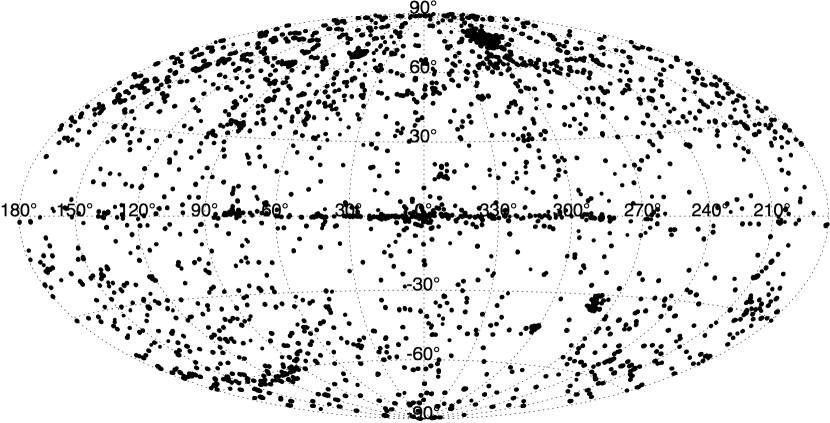
Figure 1.— Distribution of CSC release 1.0 master sources on the sky, in Galactic coordinates.

The aim of the Chandra Source Catalog (catalog ADS/Sa.CXO#CSC) (CSC) is to disseminate this wealth of information by characterizing the X-ray sky as seen by Chandra. While numerous other catalogs of X-ray sources detected by Chandra may be found in the literature (e.g., Zezas et al., 2006; Brassington et al., 2008; Romano et al., 2008; Luo et al., 2008; Muno et al., 2009; Elvis et al., 2009), the region of the sky or set of observations that comprise these catalogs is restricted, and they are typically aimed at maximizing specific scientific goals. In contrast, the CSC is intended to be an all-inclusive, uniformly processed dataset that can be utilized to address a wide range of scientific questions. The CSC is intended ultimately to comprise a definitive catalog of X-ray sources detected by Chandra, and is being made available to the astronomical community in a series of increments with increasing capability over the next several years.

The first release of the CSC was published in 2009 March. This release includes information about 135,914 source detections, corresponding to 94,676 distinct X-ray sources on the sky, extracted from a subset of public imaging observations obtained using the ACIS instrument during the first eight years of the Chandra mission. The distribution of release 1 sources on the sky is presented in Figure 1.

We expect that the CSC will be a highly valuable tool for many diverse scientific investigations. However, the catalog is constructed from pointed observations obtained using the Chandra X-ray Observatory, and is neither all-sky nor uniform in depth. The first release of the catalog includes only point and compact sources, with observed extents $\lesssim 30^{\prime\prime}$. Because of the difficulties inherent in detecting highly extended sources and point and compact sources that lie close to them, and quantifying in a consistent and robust way the properties of such sources, we have chosen to exclude entire fields (or in some cases, individual ACIS CCDs) containing such sources from the first release of the CSC, as described in § 3.1. Therefore, the catalog does not include sources near some of the most famous Chandra targets, and there may be selection effects that restrict the source content of the catalog and which therefore may limit scientific studies that require unbiased source samples.

The minimum flux significance threshold for a source to be included in the first release of the CSC is set conservatively, and corresponds typically to $\sim\!10$ detected source photons (on-axis) in the broad energy band integrated over the total exposure time. This conservative threshold was chosen to maintain the spurious source rate at an acceptable level over the wide variety of Chandra observations that are included in this release of the catalog. We expect to relax this criterion in future releases based on experience gained constructing the current release.

A number of other Chandra catalogs do include sources with fewer net counts than the CSC. Such fainter thresholds are attainable typically either because of specific attributes of the observations included in those catalogs, or because of the assumptions made when constructing the catalog.

As an example of the former category, the XBootes survey catalog (Kenter et al., 2005) includes sources that are roughly a factor of two fainter than the CSC flux significance threshold. That survey is constructed from short ($5\rm\,ks$) observations obtained in an area with low line-of-sight absorption. This results in a negligible background level that substantially simplifies source detection and enables identification of sources with very few counts. Some Chandra catalogs derived from observations with the range of exposures comparable to those that comprise the CSC (e.g., Elvis et al., 2009; Laird et al., 2009; Muno et al., 2009) also include fainter sources. However, in these cases the additional source fractions are in general not large, typically adding $\lesssim 10\%$ more sources below the CSC threshold, as described in detail in § 3.7.1.

For other Chandra catalogs, visual review and validation at the source level is a planned part of the processing thread (e.g., Kim et al., 2007; Muno et al., 2009). In some cases (e.g., Broos et al., 2007), visual review may be used to adjust processing parameters for individual sources. Such manual steps are time-consuming, but enable lower significance levels to be achieved while maintaining an acceptable spurious source rate. In contrast, the CSC catalog construction process requires that the processing pipelines run on a wide range of observations with a minimum of manual intervention. The scope of the CSC is simply too large to require manual handling at the source level. We do not manually inspect individual source detections, nor do we adjust source detection or processing parameters based on manual evaluation. Instead, the CSC uses a largely automated quality assurance approach, as described in § 3.14.

The sky coverage of the first catalog release (Fig. 2) totals $\sim\!320$ square degrees, with coverage of $\sim\!310$ square degrees brighter than a $0.5$–$7.0\rm\,keV$ flux limit of $1.0\times 10^{-13}\rm\,erg\,cm^{-2}\,s^{-1}$, decreasing to $\sim\!135$ square degrees brighter than $1.0\times 10^{-14}\rm\,erg\,cm^{-2}\,s^{-1}$, and $\sim\!6$ square degrees brighter than $1.0\times 10^{-15}\rm\,erg\,cm^{-2}\,s^{-1}$. These numbers will continue to grow as the Chandra mission continues, with a 15 year prediction of the eventual sky coverage of the CSC of order 500 square degrees, or a little over 1% of the sky.

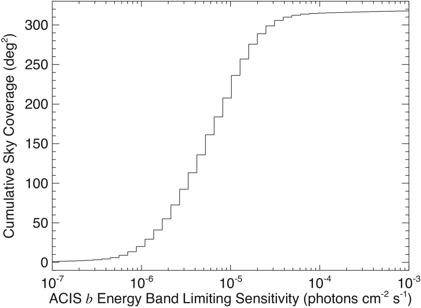
Figure 2.— Sky coverage of release 1.0 of the CSC, in the ACIS broad energy band. The ordinate value is the total sky area included in the CSC that is sensitive to point sources with fluxes at least as large as the corresponding value on the abscissa.

In this paper we describe in detail the content and construction of release 1 of the CSC. However, where appropriate we also discuss in addition the steps required to process HRC instrument data used to construct release 1.1 of the catalog, since the differences in the algorithms are small. Release 1.1 of the catalog is scheduled for spring 2010. This paper is organized into 5 sections, including the introduction. In § 2, we present a description of the catalog. This includes the catalog design goals, an outline of the general characteristics of Chandra data that are relevant to the catalog design, the organization of the data within the catalog, approaches to data access, and an outline of the data content of the catalog. Section 3, which comprises the bulk of the paper, describes in detail the methods used to extract the various source properties that are included in the catalog, with particular detail provided when the algorithms are new or have been adapted for use with Chandra data. A brief description of the principal statistical properties of the catalog sources is presented in § 4; this topic is treated comprehensively by F. A. Primini et al. (2010, in preparation). Conclusions are presented in § 5. Finally, Appendix A contains details of the algorithm used to match source detection from multiple overlapping observations, as well as the mathematical derivation of the multivariate optimal weighting formalism used for combining source position and positional uncertainty estimates from multiple observations.

2. CATALOG DESCRIPTION

2.1. Design Goals

The CSC is intended to be a general purpose virtual science facility, and provides simple access to a carefully selected set of generally useful quantities for individual sources or sets of sources matching user-specified search criteria. The catalog is designed to satisfy the needs of a broad-based group of scientists, including those who may be less familiar with astronomical data analysis in the X-ray regime, while at the same time providing more advanced data products suitable for use by astronomers familiar with Chandra data.

The primary design goals for the CSC are to (1) allow simple and quick access to the best estimates of the X-ray source properties for detected sources, with good scientific fidelity, and directly support scientific analysis using the individual source data; (2) facilitate analysis of a wide range of statistical properties for classes of X-ray sources; (3) provide efficient access to calibrated observational data and ancillary data products for individual X-ray sources, so that users can perform detailed further analysis using existing tools such as those included in the Chandra Interactive Analysis of Observations (CIAO; Fruscione et al., 2006) portable data analysis package; and (4) include all real X-ray sources detected down to a predefined threshold level in all of the public Chandra datasets used to populate the catalog, while maintaining the number of spurious sources at an acceptable level.

To achieve these goals, for each detected X-ray source the catalog records the source position and a detailed set of source properties, including commonly used quantities such as multi-band aperture fluxes, cross-band hardness ratios, spectra, temporal variability information, and source extent estimates. In addition to these traditional elements, the catalog includes file-based data products that can be manipulated interactively by the user. The primary data products are photon event lists (e.g., Conroy, 1992), which record measures of the location, time of arrival, and energy of each detected photon event in a tabular format. Additional data products derived from the photon event list include images, light curves, and spectra for each source individually from each observation in which a source is detected. The catalog release process is carefully controlled, and a detailed characterization of the statistical properties of the catalog to a well defined, high level of reliability accompanies each release. Key properties evaluated as part of the statistical characterization include limiting sensitivity, completeness, false source rates, astrometric and photometric accuracy, and variability information.

2.2. Data Characteristics

Both ACIS and HRC cameras operate in a photon counting mode, and register individual X-ray photon events. For each photon event, the two dimensional position of the event on the detector is recorded, together with the time of arrival and a measure of the energy of the event. In most operating modes, lists of detected events are recorded over the duration of an observation, typically between $1\,\rm ks$ and $160\,\rm ks$, and are then telemetered to the ground for subsequent processing.

To minimize the effect of bad detector pixels, and to avoid possible burn-in degradation of the camera by bright X-ray sources, the pointing direction of the telescope is normally constantly dithered in a Lissajous pattern, with a typical scale length of about $20^{\prime\prime}$ on the sky and a period of order $1\,\rm ks$, while taking data. The motion of the telescope is recorded via an “aspect camera” (Aldcroft et al., 2000) that tracks the motion of a set of (usually 5) guide stars as a function of time during the observation. The coordinate transformation needed to remove the motion from the event (photon) positions is computed from the aspect camera data and applied during data processing.

Breaking down the 4-dimensional X-ray data hypercube into spatial, spectral, and temporal axes provides a natural focus on the properties that may be of interest to the general user, but also identifies some of the complexities inherent in Chandra data that must be addressed by catalog construction and data analysis algorithms.

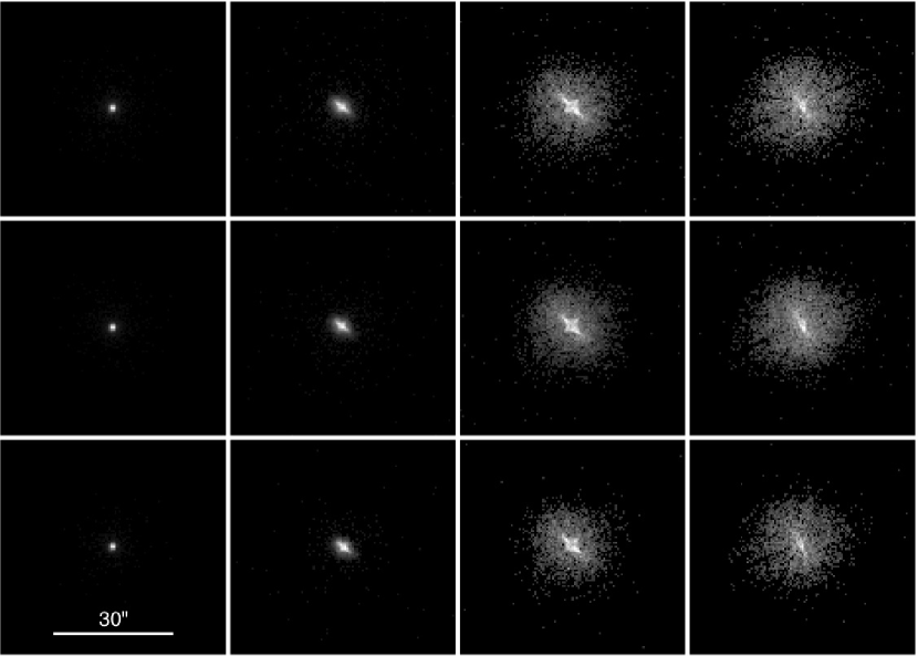
Figure 3.— Sample local Chandra model PSFs projected onto the ACIS detector pixel plane extracted from the CSC. The upper, middle, and lower sets of 4 images correspond to PSF models computed at the monochromatic effective energies of the ACIS hard, medium, and soft energy bands, respectively. From left to right, the images correspond to PSFs determined at off-axis angles $\theta=0^{\prime}$, $5^{\prime}$, $10^{\prime}$, and $15^{\prime}$, respectively. The orientation and details of the PSF substructure varies with azimuthal angle, $\phi$. The image intensity scaling is proportional to the square root of the pixel flux.

Spatially, the Chandra PSF varies significantly with off-axis and azimuthal angle (with the former variation dominating), as well as with incident photon energy (Fig. 3). Close to the optical axis of the telescope, the PSF is approximately symmetric with a 50% enclosed energy fraction radius of order $0.3^{\prime\prime}$ over a wide range of energies, but at $15^{\prime}$ off-axis the PSF is strongly energy-dependent, asymmetric, and significantly extended, with a 50% enclosed energy fraction radius of order $13^{\prime\prime}$ at $1.5\,\rm keV$.

For the widely used ACIS detector, the instrumental spectral energy resolution is of order $100$–$200\,\rm eV$, and depends on incident photon energy and location on the detector. Because the energy resolution is significantly lower than the typical energy width of the features and absorption edges that define the effective area of the telescope optics (and therefore the quantum efficiency of the telescope plus detector system), a full matrix formulation that considers the redistribution of source X-ray flux into the set of instrumental pulse height analyzer bins must be used when performing spectral analyses. This is in contrast to the more familiar scenario from many other wavebands, where the instrumental resolution is often much higher than the spectral variation of quantum efficiency, enabling the commonly used implicit assumption that the flux redistribution matrix is diagonal (and is therefore not considered explicitly).

We note in passing that Chandra is equipped with a pair of transmission gratings that can be inserted into the optical path, and is therefore capable of performing high spectral resolution (slitless spectroscopy) observations. However, such observations are not included in the current release of the CSC.

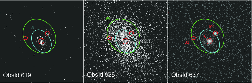
(catalog ADS/Sa.CXO#obs/00619) (catalog ADS/Sa.CXO#obs/00635) (catalog ADS/Sa.CXO#obs/00637)

Figure 4.— Three separate observations that include the area surrounding the bright X-ray source CXO J162624.0-242448 are shown. In each panel source detections from observations 00619, 00635, and 00637 are identified in cyan, green, and red, respectively. Left: Observation 00619 ($4.1\rm\,ks$ exposure). In this short exposure, only the bright source visible at an off-axis angle of $\sim\!7.7^{\prime}$. The PSF is somewhat extended. Center: Observation 00635 ($100.7\rm\,ks$ exposure). In this deep exposure, the bright X-ray source is located $\sim\!15.6^{\prime}$ off-axis in this deep exposure. The extended PSF is clearly visible. Right: Observation 00637 ($96.4\rm\,ks$ exposure). The bright source is located $\sim 3.0^{\prime}$ off-axis, and the combination of the compact PSF and long exposure resolves the region into 3 distinct source detections.

Time domain analyses must consider the impact of spacecraft dither within an observation. Strong false variability signatures at the dither frequency can arise because of variations of the quantum efficiency over the detector, or because the source or background region dithers off the detector edge or across a gap between adjacent ACIS CCDs. Corrections for these effects, as well as for cosmic X-ray background flares that can be highly variable over periods of a few kiloseconds, must be applied when computing light-curves. The extremely low photon event rates common for many faint X-ray sources typically require time domain statistics to be evaluated using event arrival-time formulations instead of rate-based approaches.

An additional level of complexity occurs because many astronomical sources of interest that will be included in the catalog are extremely faint. Rigorous application of Poisson counting statistics is required when deriving source properties and associated errors, separating X-ray analyses from many other wavebands where Gaussian statistics are typically assumed.

2.3. Data Organization

The tabulated properties included in the CSC are organized conceptually into two separate tables, the Source Observations Table and the Master Sources Table. Distinguishing between source detections (as identified within a single observation) and X-ray sources physically present on the sky is necessary because many sources are detected in multiple observations and at different off-axis angles (and therefore have different PSF extents).

Each record included in the Source Observations Table tabulates properties derived from a source detection in a single observation. These entries also include pointers to the associated file-based data products that are included in the catalog, which are all observation-specific in the first catalog release. Each record in the Source Observations Table is further split internally into a set of source-specific data and a set of observation-specific, but source-independent, data. The latter are recorded once to avoid duplication. A description of the data columns recorded in the Source Observations Table for each source detection is provided in Table 1.

Because of the dependence of the PSF extent with off-axis angle, multiple distinct sources detected on-axis in one observation may be detected as a single source if located far off-axis in a different observation (Fig. 4). During catalog processing, source detections from all observations that overlap the same region of the sky are spatially matched to identify distinct X-ray sources. Estimates of the tabulated properties for each distinct X-ray source are derived by combining the data extracted from all source detections and observations that can be uniquely associated, according to the algorithms described in § 3. The best estimates of the source properties for each distinct X-ray source are recorded in the Master Sources Table. A description of the data columns recorded in the Master Sources Table for each source is provided in Table 2.

Each distinct X-ray source is thus conceptually represented in the catalog by a single entry in the Master Sources Table, and one or more associated entries in the Source Observations Table (one for each observation in which the source was detected).

All of the tabulated properties included in both the Master Sources Table and the Source Observations Table can be queried by the user. Bi-directional links between the entries in the two tables are managed transparently by the database, so that the user can access all observation data for a single source seamlessly.

If a source detection included in the Source Observations Table can be related unambiguously to a single X-ray source in the Master Sources Table, then the corresponding table entries will be associated by “unique” linkages. Source detections included in the Source Observations Table that cannot be related uniquely to a single X-ray source in the Master Source Table will have their entries associated by “ambiguous” linkages (Fig. 5).

Figure 5.— Linkages between the Master Sources Table and the Source Observations Table entries for the source detections from Fig. 4 are depicted. The 3 source detections in observation 00637 are uniquely identified with distinct X-ray sources on the sky, and will be associated with the corresponding master sources through “unique” linkages. Similarly, the single source detection (region 5) in observation 00619 is an unambiguous match to region 6 in observation 00637, and so will also be associated with the same master source via a unique linkage. The confused detection, region 99 in observation 00635 overlaps the 3 source detections in observation 00637, and so is associated with the corresponding master sources with “ambiguous” linkages.

The data from ambiguous source detections are not used when computing the best estimates of the source properties included in the Master Sources Table. In the case of ACIS observations, source detections for which the estimated photon pile-up fraction (Davis, 2007a) exceeds $\sim\!10\%$ will not be used if source detections in other ACIS observations do not exceed this threshold.

Using the linkages between the entries in the two tables, the user will nevertheless be able to identify all of the X-ray sources in the catalog that could be associated with a specific detection in a single observation, and vice-versa. These linkages may be important, for example, when identifying candidate targets for follow-up studies based on a data signature that is only visible in the observation data for a confused source.

2.4. Data Access

The primary user tool for querying the CSC is the CSCview web-browser interface (Zografou et al., 2008), which can be accessed from the public catalog web-site. The user can directly query any of the tabulated properties included in either the Master Sources Table or the Source Observations Table, display the contents of an arbitrary set of properties for matching sources, and retrieve any of the associated file-based data products for further analysis. CSCview provides a form-based data-mining interface, but also allows users to enter queries written using the Astronomical Data Query Language (ADQL; Ortiz et al., 2008) standard directly. Query results can be viewed directly on the screen, or saved to a data file in multiple formats, including tab-delimited ASCII (which can be read directly by several commonly used astronomical applications) and International Virtual Observatory Alliance (IVOA) standard formats such as VOTable (Ochsenbein, 2009).

Automated access to query the catalog from data analysis applications and scripts running on the user’s home platform was identified as being needed for several science use cases. VO standard interfaces, including Simple Cone Search (Williams et al., 2008) and Simple Image Access (Tody & Plante, 2009), provide limited query and data access capabilities, while more sophisticated interactions are possible through a direct URL connection. Support for VO workflows using applicable standards will be added in the future as these standards stabilize. An interface that integrates catalog access with a visual sky browser provides a simple mechanism for visualizing the regions of the sky included in the catalog, and may also be particularly beneficial for education and public outreach purposes.

Since Chandra is an ongoing mission, the CSC includes a mechanism to permit newly released observations to be added to the catalog and be made visible to end users, while at the same time providing stable, well-defined, and statistically well-characterized released catalog versions to the community. This is achieved by maintaining a revision history for each database table record, together with flags that establish whether catalog quality assurance and catalog inclusion criteria are met, and using distinct views of the catalog databases that utilize these metadata.

“Catalog release views” provide access to each released version of the catalog, with the latest released version being the default. Catalog releases will be infrequent (no more than of order 1 per year) because of the controls built in to the release process, and because of the requirement that each release be accompanied by a detailed statistical characterization of the included source properties. Once data are included in a catalog release view, then they are frozen in that view, even if the source properties are revised or the source is deleted in a later catalog release. A source may be deleted if the detection is subsequently determined to be an artifact of the data or processing, but the most likely reason that a source is deleted from a later catalog release is that additional observations included in the later release resolve the former detection into multiple distinct sources.

Table 4CSC Energy Bands

Band		Energy	Monochromatic	Integrated Effective Area
Name	Designation	Range	Energy	ACIS-I	ACIS-S	HRC-I
ACIS Energy Bands
Ultra-soft	u	0.2–0.5	0.40	7.36–2.24	68.7–23.0	$\cdots$
Soft	s	0.5–1.2	0.92	216–155	411–274	$\cdots$
Medium	m	1.2–2.0	1.56	438–401	539–493	$\cdots$
Hard	h	2.0–7.0	3.80	1590–1580	1680–1670	$\cdots$
Broad	b	0.5–7.0	2.30	2240–2140	2630–2440	$\cdots$
HRC Energy Band
Wide	w	0.1–10	1.50	$\cdots$	$\cdots$	605

“Database views” provide access to the catalog database, including any new content that may not be present in an existing catalog release. Because on-going processing is continually modifying the catalog database, tabulated data and file-based data products in a database view may be superseded at any time, and the statistical properties of the data are not guaranteed.

We anticipate that users who require a stable, well-characterized dataset will choose primarily to access the catalog through the latest catalog release view. On the other hand, users who are interested in searching the latest data to identify sources with specific signatures for further study will likely use the latest database view.

2.5. Data Content

The first release of the CSC includes detected sources whose flux estimates are at least 3 times their estimated $1\,\sigma$ uncertainties, which typically corresponds to about 10 net (source) counts on-axis and roughly 20–30 net counts off-axis, in at least one energy band. In this release, multiple observations of the same field are not combined prior to source detection, so the flux significance criterion applies to each observation separately.

For each source detected in an observation, the catalog includes approximately 120 tabulated properties. Most values have associated lower and upper confidence limits, and many are recorded in multiple energy bands. The total number of columns included in the Source Observations Table (including all values and associated confidence limits for all energy bands) is 599.

Roughly 60 master properties are tabulated for each distinct X-ray source on the sky, generated by combining measurements from multiple observations that include the source. Combining all values and associated confidence limits for all energy bands yields a total of 287 columns included in the Master Sources Table.

The tabulated source properties fall mostly into the following broad categories: source name, source positions and position errors, estimates of the raw (measured) extents of the source and the local point spread function, and the deconvolved source extents, aperture photometry fluxes and confidence intervals measured or inferred in several ways, spectral hardness ratios, power-law and thermal black-body spectral fits for bright ($>150$ net counts) sources, and several source variability measures (Gregory-Loredo, Kolmogorov-Smirnov, and Kuiper tests).

Also included in the CSC are a number of file-based data products in formats suitable for further analysis in CIAO. These products, described in Table 3, include both full-field data products for each observation, and products specific to each detected observation-specific source region.

The full-field data products include a “white-light” full-field photon event list, and multi-band exposure maps, background images, exposure-corrected and background-subtracted images, and limiting sensitivity maps.

Source-specific data products include a white-light photon event list, the source and background region definitions, a weighted ancillary response file (the time-averaged product of the combined telescope/instrument effective area and the detector quantum efficiency), multi-band exposure maps, images, model ray-trace PSF images, and optimally binned light-curves. Observations obtained using the ACIS instrument additionally include low-resolution ($E/{\Delta E}\sim\!10$–$40$, depending on incident photon energy and location on the array) source and background spectra and a weighted detector redistribution matrix file (the probability matrix that maps photon energy to detector pulse height).

2.5.1 Energy Bands

The energy bands used to derive many CSC properties are defined in Table 4. The energy bands are chosen to optimize the detectability of X-ray sources while simultaneously maximizing the discrimination between different spectral shapes on X-ray color-color diagrams.

The effective area of the telescope (including both the Chandra High Resolution Mirror Assembly [HRMA] and the detectors) is shown in Figure 6 as a function of energy, together with the average ACIS quiescent backgrounds derived from blank sky observations (Markevitch, 2001a). The effective area is measured at the locations of the nominal “ACIS-S” aimpoint on the ACIS S3 CCD, and the nominal “ACIS-I” aimpoint on the ACIS I3 CCD.

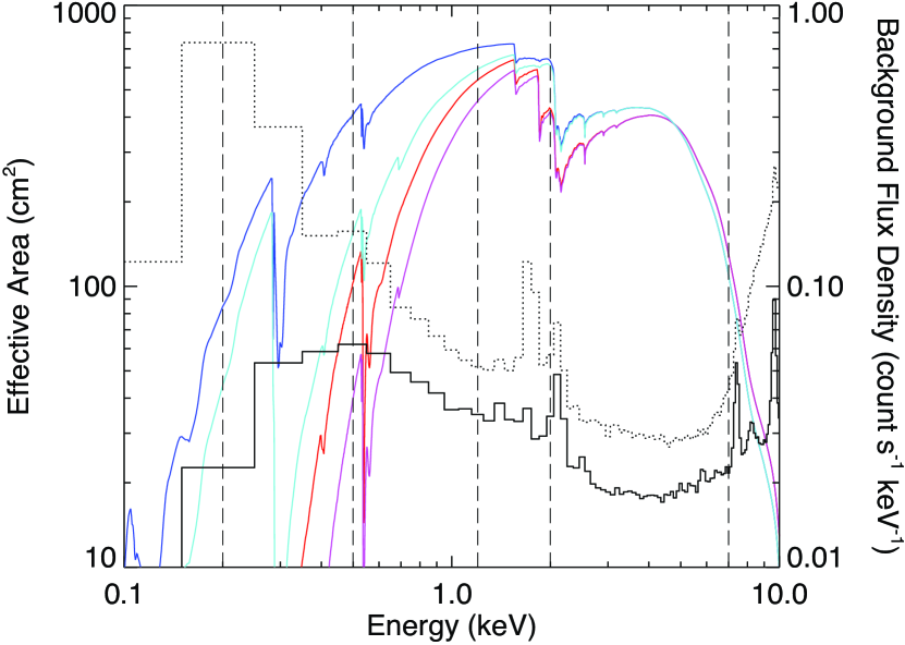
Figure 6.— Chandra effective area and average ACIS quiescent background as a function of energy. The blue and cyan curves present the combined HRMA plus ACIS effective area at the ACIS-S aimpoint, with zero and the late 2009 level of focal plane contamination, respectively. The red and cyan curves show the effective area at the ACIS-I aimpoint, again with zero and late 2009 contamination, respectively. The dotted black line shows the quiescent background flux density on the ACIS S3 CCD, while the solid black line represents the ACIS I3 CCD background. The energies corresponding to the edges of the CSC energy bands are shown by vertical dashed lines.

Where possible, the energy bands are chosen to avoid large changes of effective area within the central region of the band, since such variations degrade the accuracy of the monochromatic effective energy approximation described below. For example, the M-edge of the Iridium coating on the HRMA has significant structure in the $\sim\!2.0$–$2.5\rm\,keV$ energy range that provides a natural breakpoint between the ACIS medium and hard energy bands. Note however, that large effective area variations are unavoidable within the ACIS broad and soft energy bands and the HRC wide energy band.

Weighting the effective area by the source spectral shape and integrating over the bandpass provides an indication of the relative detectability of a source in the energy band. Selecting energy band boundaries so that source detectability is roughly the same in different energy bands more uniformly distributes Poisson errors across the bands, and so enhances detectability in the various bands.

Several different source types were simulated when selecting energy bands. These included absorbed non-thermal (power-law) models with photon index values ranging from 1 to 4, absorbed black-body models with temperature varying from $20\rm\,eV$ to $2.0\rm\,keV$, and absorbed, hot, optically-thin thermal plasma models (Raymond & Smith, 1977) with $kT=0.25$–$4.0\rm\,keV$. In all cases, the Hydrogen absorbing column was varied over the range $1.0\times 10^{20}$–$1.0\times 10^{22}\rm\,cm^{-2}$. Detected X-ray spectra were simulated using PIMMS (Mukai, 2009), and then folded through the bandpasses to construct synthetic X-ray color-color diagrams (see Fig. 7 for example color-color diagrams based on the final band parameters). Energy bands chosen to fill the color-color diagrams maximally provide the best discrimination between different spectral shapes. For detailed X-ray spectral-line modeling, the Raymond & Smith (1977) models have been superseded by more recent X-ray plasma models (e.g., Mewe et al., 1995; Smith et al., 2001). However, since the radiated power of the newer models as a function of temperature is not significantly different from the 1993 versions of the Raymond & Smith (1977) models used here, the latter are entirely adequate for the purpose of evaluating coverage of the X-ray color-color diagrams and the task is greatly simplified because of their availability in PIMMS.

Grimm et al. (2009) compared broad band X-ray photometry with accurate ACIS spectral fits and found that model-independent fluxes could be derived from the photometry measurements to an accuracy of about 50% or better for a broad range of plausible spectra. They used similar but not identical energy bands to those adopted for the CSC, but did not use the method of deriving fluxes from individual photon energies employed herein.

Combining all of these considerations (McCollough, 2007) yields the following selection of energy bands for the CSC.

The ACIS soft (s) energy band spans the energy range 0.5–$1.2\rm\,keV$. The lower bound is a compromise that is set by several considerations. ACIS calibration uncertainties increase rapidly below $0.5\rm\,keV$, so this establishes a fairly hard lower limit to avoid degrading source measurements in the energy band. As shown in Figure 8, below about $0.6\rm\,keV$ the background count rate begins to increase rapidly, while the integrated effective area rises very slowly resulting in few additional source counts. While pushing the band edge to higher energy will result in a lower background, the integrated effective area drops rapidly if the lower bound is raised above $\sim\!0.8\rm\,keV$, reducing the number of source counts collected in the band. We choose to set the lower bound equal to $0.5\rm\,keV$ since doing so enhances the detectability of super-soft sources, while not noticeably impacting measurements of other sources. The upper cutoff for the soft energy band is set equal to $1.2\,\rm keV$, which balances the preference for uniform integrated effective areas amongst the energy bands with the desire to maximize the area of X-ray color-color plot parameter space spanned by the simulations.

The lower bound of the ACIS medium (m) energy band matches the upper bound of the soft energy band. We locate the upper band cutoff at $2.0\rm\,keV$ since this value tends to maximize the coverage of the X-ray color-color diagram. This value also moves the Iridium M-edge out of the sensitive medium band, and instead placing it immediately above the lower boundary of the ACIS hard (h) energy band.

The high energy boundary of the latter band is set to $7.0\rm\,keV$. This cutoff provides a good compromise between maximizing integrated effective area and minimizing total background counts (Fig. 8). Above $7.0\rm\,keV$, the background rate increases rapidly at the ACIS-S, while below this energy the integrated effective area decreases rapidly at the ACIS-I aimpoint. Placing the hard energy band cutoff at $7.0\rm\,keV$ also has the advantage that the $\rm Fe\,K\alpha$ line is included in the band, allowing intense Fe line sources to be detected without compromising the measurement quality for typical catalog sources.

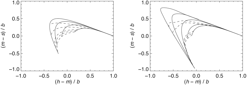
Figure 7.— Synthetic color-color diagrams computed for the ACIS hard ($h$), medium ($m$), soft ($s$), and broad ($b=h+m+s$) energy bands. Left: Absorbed power-law models. The solid lines are lines of constant photon index $\Gamma=1.0$, $2.0$, $3.0$, and $4.0$ (from right to left). The dashed lines are lines of constant neutral Hydrogen column densities $N_{\rm H}=1.0\times 10^{20}$, $1.0\times 10^{21}$, $2.0\times 10^{21}$, $5.0\times 10^{21}$, and $1.0\times 10^{22}\rm\,cm^{-2}$ (from bottom to top). Right: Hot, optically thin thermal plasma models (Raymond & Smith, 1977). The solid lines are lines of constant temperature $kT=0.25$, $0.5$, $1.0$, $2.0$, and $4.0\rm\,keV$ (from left to right). The dashed lines are lines of constant neutral Hydrogen column densities $N_{\rm H}=1.0\times 10^{20}$, $1.0\times 10^{21}$, $2.0\times 10^{21}$, $1.4\times 10^{22}$, and $1.75\times 10^{22}\rm\,cm^{-2}$ (from bottom to top). Energy bands were chosen to optimize the ability to estimate spectral parameters from color-color diagrams.

The ACIS broad (b) band covers the same energy range as the combined soft, medium, and hard bands, and therefore spans the energy range 0.5–$7.0\rm\,keV$.

Simulations indicate that an additional energy band extending below $0.5\,\rm keV$ is beneficial for discriminating super-soft X-ray sources in color-color plots. The ACIS front-illuminated CCDs have minimal quantum efficiency below $0.3\,\rm keV$, while the response of the back-illuminated CCDs extends down to $\sim 0.1\,\rm keV$. Hydrocarbon contamination is present on both the HRMA optics (Jerius, 2005) and the ACIS optical blocking filter (Marshall et al., 2004). The latter reduces the effective area at low energies, and enhances the depth of the Carbon K-edge. An ACIS ultra-soft (u) band covering $0.2$–$0.5\,\rm keV$ is added to provide better discrimination of super-soft sources. Source detection is not performed in this energy band, because of the typical lower overall signal-to-noise ratio (SNR) and the resulting enhanced false-source rate.

Finally, since the HRC (particularly HRC-I) has minimal spectral resolution, a single wide (w) band that includes essentially the entire pulse height spectrum (specifically, PI values $0:254$), roughly equivalent to 0.1-10 keV, is used for HRC observations.

While bands in these general energy ranges give the best balance of count rate and spectral discrimination, our simulations indicate that the exact choice of band boundary energies is not critical at the 10% level.

2.5.2 Band Effective Energies

In principle, the variations of HRMA effective area, detector quantum efficiency, and (for ACIS) focal plane contamination, with energy imply that energy-dependent data products such as exposure maps or PSFs should be constructed by integrating the source spectrum over the energy band. This approach would be both extremely time-consuming, and require knowledge of the source spectrum that is typically not available a priori. In practice, a monochromatic effective energy is chosen for each energy band to be used to construct energy dependent data products (McCollough, 2007).

The monochromatic effective energy for each band is determined using the relation

$$E_{\rm eff}=\frac{\int dE\,EA(E)Q(E)C(E)S(E)}{\int dE\,A(E)Q(E)C(E)S(E)},$$ (1)

where $E$ is the energy, $A$ is the effective area of the HRMA, $Q$ is the detector quantum efficiency, $C$ is the reduction in transmission due to focal plane contamination, $S$ is a power-law spectral weighting function of the form $(E/E_{0})^{-\alpha}$, and the integral is performed over the energy band.

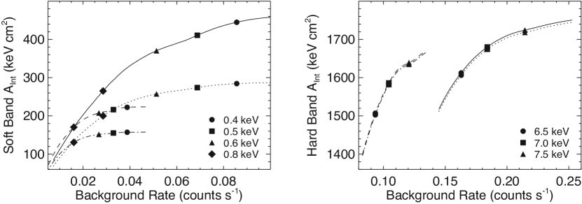
Figure 8.— Left: Plot shows how the ACIS soft (s) energy band integrated effective area and background count rate per CCD vary with the choice of lower bound for the energy band. Markers for different lower bounds are shown. The individual curves show the relationship at the ACIS-S and ACIS-I aimpoints, and with zero and the late 2009 level of focal plane contamination, as follows. Solid line: ACIS-S aimpoint, no contamination; dotted line: ACIS-S aimpoint, late 2009 contamination; dashed line: ACIS-I aimpoint, no contamination; dash-dotted line: ACIS-I aimpoint, late 2009 contamination. Right: Plot shows how the ACIS hard (h) energy band integrated effective area and background count rate per CCD vary with the choice of upper bound for the energy band. Markers and line styles are the same as in the left panel.

The monochromatic effective energies for each energy band were calculated for sources located at the ACIS-I and ACIS-S aimpoints, and also for the nominal aimpoint on the HRC-I detector. Since the CSC is constructed from observations acquired throughout the Chandra mission, ACIS focal plane contamination models with both zero contamination (appropriate for observations obtained early in the mission) and the contamination level current as of late 2009 were employed. Power-law spectral weighting functions with $\alpha$ varying from 0.0 to 2.0 were used. Setting $\alpha=1$ gives a spectral weighting function that approximates an absorbed $\Gamma=1.7$ power-law spectrum, and the limits for $\alpha$ were chosen to span the typical range of values determined from fits to a canonical subset of Chandra datasets. The remaining parameters in equation (1) are extracted from the Chandra calibration database (CalDB; George & Corcoran, 2005; Graessle et al., 2006). The monochromatic effective energies for ACIS were chosen to be the approximate arithmetic means of the $\alpha=1$ values derived for the ACIS-I and ACIS-S aimpoints, with zero and late 2009 focal plane contamination. For ACIS energy bands other than the the broad band, the monochromatic effective energies computed for a single value of $\alpha$ all agree within $\lesssim 0.1\rm\,keV$. The dependence on $\alpha$ is similarly small, except for the hard energy band, where varying $\alpha$ from 0.0 to 2.0 changes the monochromatic effective energy from $\sim\!4.2\rm\,keV$ to $\sim\!3.4\rm\,keV$. For the ACIS broad energy band, the agreement between the different models for a single value of $\alpha$ is $\sim\!\pm 0.3\rm\,keV$. However, for this band the dependence on $\alpha$ is more significant, varying from $\sim\!3.3\rm\,keV$ for $\alpha=0.0$ to $\sim\!1.6\rm\,keV$ for $\alpha=2.0$. The monochromatic effective energies used to construct the CSC are reported in Table 4.

Although the use of a single monochromatic effective energy for each energy band simplifies data analysis by removing the dependence on the source spectrum, some error will be introduced for sources that have either extremely soft or extremely hard spectra compared to the canonical $\alpha=1.0$ power-law spectral weighting function. Knowledge of the expected magnitude of the error that may be introduced is helpful when evaluating catalog properties.

For both the ACIS medium and hard energy bands, neither extremely soft nor extremely hard source spectra induce variations in exposure map levels that are greater than $\sim\!10\%$, so photometric errors due to source spectral shape should not exceed this value. In the ACIS soft energy band, very soft spectra may produce deviations of order 5–20%, with the largest excursions expected for the front-illuminated CCDs. These differences increase to $\sim\!15$–35% for the ACIS ultra-soft energy band, with the largest values once again associated with the front-illuminated CCDs. For all of the ACIS narrow energy bands, the errors induced by extremely hard spectra are much smaller than those caused by extremely soft spectra. The presence of the Iridium edge and the large energy ranges included in the ACIS broad and HRC wide energy bands may produce significantly larger variations for extreme spectral shapes. Very soft spectra can alter exposure map values by $\sim\!65$–90% in the ACIS broad energy band, although there is little impact in the HRC wide energy band. Conversely, extremely hard spectra may induce changes up to $\sim\!70\%$ in the HRC wide energy band, and $\sim\!25$–30% in the ACIS broad energy band. As described in § 4.4, model-based statistical characterization of CSC source fluxes (F. A. Primini et al. 2010, in preparation) produces results that are generally consistent with these expectation, with the exception that flux errors in the ACIS broad energy band appear to be $\sim\!10\%$ for most sources.

When computing fluxes for point sources, an aperture correction is applied to compensate for the fraction of the PSF that is not included in the aperture. Since the extent of the Chandra PSF varies with energy, using a monochromatic effective energy can introduce a flux error because the energy dependence of the PSF fraction is not considered. This error can be bounded by a post facto comparison of PSF fractions for catalog source detections in the 5 ACIS energy bands. The majority of variations between energy bands fall in the range 4–8%, with 90% of source detections showing $<10\%$ differences. These values represent an upper bound on the error introduced within an energy band by the use of a monochromatic effective energy.

2.5.3 Coordinate Systems and Image Binning

As described previously, X-ray photon event data are recorded in the form of a photon event list. The pixel position on the detector where a photon was detected is recorded in the “chip” pixel coordinate system. Event positions are remapped to celestial coordinates through a series of transforms, as described by McDowell (2001). The first step in this process remaps chip coordinates to a uniform real-valued virtual “detector” pixel space by applying corrections for the measured detector geometry, and instrumental and telescope optical system distortions recorded in the CalDB. Subsequent application of the time-dependent aspect solution removes the spacecraft dither motion, and maps the event positions to a uniform virtual “sky” pixel plane. The latter has the same pixel scale as the original instrumental pixels, but is oriented with North up ($+Y$ direction) and is centered at the celestial coordinates of the tangent plane position for the observation. As an aid to users, the location of each event in each coordinate system is recorded in the calibrated photon event list. A simple unrotated world coordinate system transform maps sky positions to ICRS right ascension and declination by applying the plate scale calibration to the difference between the position of the source and a fiducial point, which is typically the optical axis of the telescope. The celestial coordinates of the fiducial point are determined from the aspect solution.

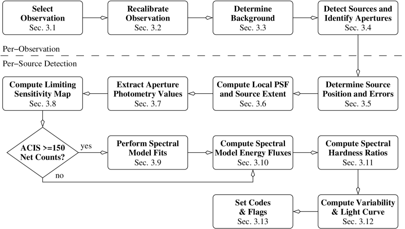
Figure 9.— High-level flow diagram depicting the steps used to process each observation’s full field-of-view, detect sources, and extract the physical properties for each detected source. The references identify the relevant sections of the text that describe in detail the methods used.

Sky images are constructed from the calibrated photon event lists by binning photon positions in sky coordinates into a regular, rectangular image pixel grid. A consequence of constructing images by binning in sky coordinates is that Chandra images are always oriented with North up. The choice of image blocking factor determines the number of sky pixels that are binned into a single image pixel. Full field image products associated with ACIS observations are constructed by binning the area covered by the inner $2048\times 2048$ sky pixels at single pixel resolution, then binning the inner $4096\times 4096$ sky pixels at block 2, and finally binning the entire $8192\times 8192$ sky pixel field at block 4. The corresponding blocking factors for HRC-I observations are 2, 5, and 12. Using a constant blocked image size of $2048\times 2048$ pixels reduces overall data volume, while preserving resolution in the outer areas of the field of view where the PSF size is significantly larger than a single pixel.

3. CATALOG GENERATION

In this section, we describe in detail the methods used to derive the X-ray source properties that are included in the CSC, with particular detail provided in cases where the algorithms are new or have been newly adapted for use with Chandra data.

The principal steps necessary to generate the catalog consist of processing the data for each observation’s full field-of-view, detecting X-ray sources included within that field of view, and then extracting the spatial, photometric, spectral, and temporal properties of each detected source. Figure 9 is a depiction of the high-level flow used to perform these steps. In the figure, each block references the section of the text that describes in detail the methods used. The physical properties associated with each source detection are recorded as a separate row in the catalog Source Observations Table.

Once the source detections from each observation have been evaluated, they are correlated with source detections from all other spatially overlapping observations to identify distinct X-ray sources on the sky. The steps required to perform the source cross-matching, and then combine the data from multiple observations of a single source to evaluate the source’s properties, follow a similar flow to the one presented in Figure 10. Many of the elements that comprise the second flow are built on the foundations developed for the related steps from the first flow. For convenience and continuity of notation, the former are described in the same text sections as the latter. The properties for each distinct X-ray source are included as a separate row in the catalog Master Sources Table.

Data processing for release 1 of the CSC was performed using versions 3.0–3.0.7 of the Chandra X-ray Center data system (CXCDS; Evans et al., 2006a, b) catalog processing system (“CAT”), with calibration data extracted from CalDB version 3.5.0. The observation recalibration steps included in CAT3.0 correspond approximately with those included CIAO 4.0. In several cases, programs developed for CAT3.0 to evaluate source properties have been repackaged with new interfaces for interactive use in subsequent CIAO releases (see Table 5).

3.1. Observation Selection

While the CSC ultimately aims to be a comprehensive catalog of X-ray sources detected by Chandra, all of the functionality required to achieve that goal are not included in the release 1 processing system. A set of pre-filters is used to limit the data content to the set of observations that the catalog processing system is capable of handling.

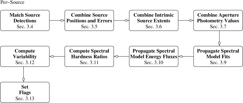
Figure 10.— As Fig. 9, except that the steps used to cross-match source detections, and combine data from multiple observations to evaluate source properties, are shown.

For release 1, only public ACIS “timed-exposure” readout mode imaging observations obtained using either the “faint,” “very faint,” or “faint with bias” datamodes are included. ACIS observations that are obtained using CCD subarrays with $\leq 128$ rows are also excluded, because there are too few rows to ensure that source-free regions can be identified reliably when constructing the high spatial frequency background map. HRC-I imaging mode observations are not included in release 1 of the catalog, but are included in incremental release 1.1. HRC-S observations are excluded because of the presence of background features associated with the edges of “T”-shaped energy-suppression filter regions that form part of the UV/ion-shield. Observations of solar system objects are not included in the CSC.

All observations included in the CSC must have been processed using the standard data processing pipelines included in version 7.6.7, or later, of the CXCDS. This version of the data system was used to perform the most recent bulk reprocessing of Chandra data, and includes revisions to the pipelines that compute the aspect solution that is used to correct for the spacecraft dither motion and register the source events on the sky. Observations must have successfully passed the “validation and verification” (quality assurance) checks that are performed upon completion of standard data processing.

The largest scale lengths used to detect sources to be included in the CSC have angular extents $\sim\!30^{\prime\prime}$. Sources with apparent sizes greater than this are either not detected, or may be detected incorrectly as multiple close sources. Prior to catalog construction, all observations are inspected visually for the presence of extended sources that may be detected incorrectly, and such observations are excluded from catalog processing. For ACIS observations, if the presence of any spatially extended emission is restricted to a single CCD only, then the data from that CCD are dropped, and sources detected on any remaining CCDs are typically included in the catalog. The latter rule allows many sources surrounding bright, extended cores of galaxies to be included in the catalog, rather than having the entire observation rejected outright.

While the visual inspection and rejection process is inherently subjective in nature, an attempt was made to calibrate the method by constructing a “training set” of several hundred observations that were processed through a test version of the catalog pipelines. The training set observations included a wide variety of point, compact, and extended sources, with differing exposures and SNR, which were classified as accept/reject based on the actual results of running the pipeline source detection and source property extraction steps. These observations and classifications were then used to train the personnel who performed the visual inspection process.

3.2. Observation Recalibration

Although all observations included in the CSC have been processed through the CXCDS standard data processing pipelines, we nevertheless re-run the instrument-specific calibration steps as the first step in catalog construction. One reason for reapplying the instrumental calibrations is that they are subject to continuous improvements, and may have been revised since the last time the observations were processed or reprocessed. A second reason is to ensure that a single set of calibrations are applied to all datasets, so that the resulting catalog will be calibrated as homogeneously as possible.

For ACIS, the principal instrument-specific calibrations that are re-applied are the (time-dependent) gain calibration and the correction for CCD charge transfer inefficiency (CTI). The former calibration maps the measured pulse height for each detected X-ray event into a measurement of the energy of the corresponding incident X-ray photon. CTI correction attempts to account for charge lost to traps in the CCD substrate when the charge is being read out. This effect is considerably larger than anticipated prior to launch because of damage to the ACIS CCDs caused by the spacecraft’s radiation environment. Additionally, observation-specific bad pixels and hot pixels are flagged for removal, as are “streak” events on CCD S4 (ACIS-8). The latter apparently result from a flaw in the serial readout electronics (Houck, 2000). Pixel afterglow events, which arise because of energy deposited into the CCD substrate by cosmic ray charged particles, are removed using the acis_run_hotpix tool that is also included in CIAO. Although this program can miss some real faint afterglows, such events are very unlikely to exceed the flux significance threshold required for inclusion in the catalog. The default 0.5 pixel event position randomization in chip coordinates is used when the calibrations are reapplied.

Table 5CSC-Related CIAO Tools

Tool Name	CIAO Version	Description
aprates	4.1	Calculate source aperture photometry properties
dmellipse	4.1	Calculate ellipse including specified encircled fraction
eff2evt	4.1	Calculate energy flux from event energies
lim_sens	4.1	Create a limiting sensitivity map
mkpsfmap	4.1	Look up PSF size for each pixel in an image
acis_streak_map	4.1.2	Create a high spatial frequency background map
dither_region	4.1.2	Calculate region on detector covered by a sky region
evalpos	4.1.2	Get image values at specified world coordinates
glvary	4.1.2	Search for variability using Gregory-Loredo algorithm
pileup_map	4.1.2	Create image that gives indication of pileup
modelflux	4.1.2	Calculate spectral model energy flux
srcextent	4.1.2	Compute source extent
create_bkg_map	4.2	Create a background map from event data
dmimgpm	4.2	Create a low spatial frequency background map

The main instrument specific calibrations for HRC data relate to the “degapping” correction that is applied to the raw X-ray event positions to compensate for distortions introduced by the HRC detector readout hardware. Several additional calibrations compensate for effects introduced by amplifier range switching and ringing in the HRC electronics, and a number of validity tests are performed to flag X-ray event positions that cannot be properly corrected due to amplifier saturation and other effects.

Since data are recorded continuously during an observation, a “Mission Time Line” is constructed during standard data processing that records the values of key spacecraft and instrument parameters as a function of time. These parameters are compared with a set of criteria that define acceptable values, and “Good Time Intervals” (GTIs) that include scientifically valid data are computed for the observation. The GTI filter from standard data processing is reapplied without change as part of the recalibration process.

Background event screening performed as part of catalog data recalibration is somewhat more aggressive than that performed as part of standard data processing, typically reducing the non-X-ray background. For a $10\rm\,ks$ observation, the median catalog background rate is roughly 80% of the nominal field background rates (Chandra X-ray Center, 2009), although there is considerable scatter. F. A. Primini et al. (2010, in preparation) include a detailed statistical analysis of the improvements to the non-X-ray background afforded by this screening.

The reduction of the background event rate is achieved by removing time intervals containing strong background flares. These time intervals are identified separately for each chip. First, the background regions of the image are identified by constructing a histogram of the event data, determining the mean and standard deviations of the histogram values, and rejecting all pixels that have values more than 3 standard deviations above the mean. An optimally-binned light curve of the background pixels is then created using the Gregory-Loredo algorithm (see § 3.12.1). Time bins for which the count rate exceeds $10\times$ the minimum light curve value are identified. The corresponding intervals are considered to be background flares, and the GTIs are revised to exclude those periods.

We emphasize that the objective of this procedure is to remove only the most intense background flares, which occur relatively infrequently. Time intervals that include moderately enhanced background rates are not rejected by this process, since their contributions increase the overall SNR. The aggregate loss of good exposure time exceeds 25% for less than 1.5% of the observations included in the catalog; the loss is greater than 10% for 3% of the observations, and greater than 5% for 5% of the observations.

For each observation included in the CSC, the recalibrated photon event list is archived, together with several additional full-field data products. These include multi-resolution exposure maps computed at the monochromatic effective energies of each energy band and the associated ancillary data products (aspect histogram, bad pixel map, and field of view region definition), used to construct them (see Table 3).

3.3. Background Map Creation

For the first release of the CSC, background maps are used for automated source detection. They are created directly from each individual observation with the necessary accuracy. The general observation background is assumed to vary smoothly with position, and is modeled using a single low spatial frequency component. Although this assumption is in general satisfied across the fields of view included in this catalog release, there may be localized regions where the background intensity has a strong spatial dependence, and therefore where the detectability of sources may be reduced. Several different approaches were considered for constructing the low spatial frequency background component, including spatial transforms, low pass filters, and data smoothing. However, the most effective and physically meaningful technique is a modified form of a Poisson mean. This method, described below, estimates the local background from the peak of the Poisson count distribution included in a defined sampling area. The dimensions of the sampling area act effectively as a spatial low pass filter that determines the minimum angular size that contributes to the background.

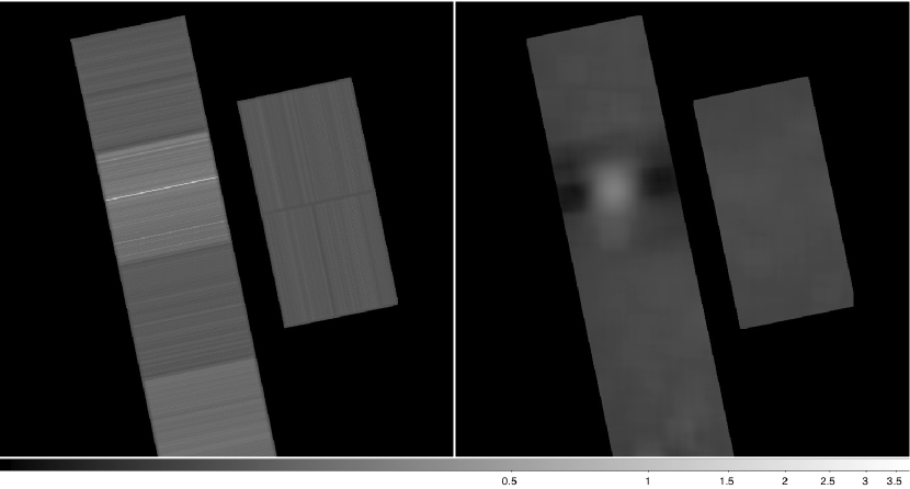
Figure 11.— ACIS broad-band high and low spatial frequency background maps for observation 00735, as used for catalog source detection (Fig. 12, Right). Left: ACIS high spatial frequency background map component. Each image pixel represents $2\times 2$ blocked sky pixels. Intensities have an an offset of $+0.1\,\hbox{\rm count}\,\hbox{\rm(image pixel)}^{-1}$ added, and the result is scaled logarithmically over the range 0.0375–3.75. The readout streak associated with the bright source is clearly visible. Right: ACIS low spatial frequency background map component. The Poisson mean includes a residual image of the bright source, at a peak level of $\sim\!0.15\,\hbox{\rm count}\,\hbox{\rm(image pixel)}^{-1}$.

High spatial frequency linear features, commonly referred to as “readout streaks,” result when bright X-ray sources are observed with ACIS. These streaks arise from source photons that are detected during the CCD readout frame transfer interval ($\sim\!40\,\mu\rm s$ per row) following each exposure ($\sim\!3.2\,\rm s$ per exposure for a typical observation). All pixels along a given readout column are effectively exposed to all points on the sky that lie along that column during the frame transfer interval, so that columns including bright X-ray sources have enhanced count rates along their length. Unless accounted for by the source detection step, the increased counts in the bright readout streak are detected as multiple sources. Although readout streaks are comprised of mis-located source photons, we choose to model them as a background component.

Background maps computed for ACIS observations include contributions from both components, while HRC background maps include only the low spatial frequency component.

The reader should note that background maps are not used when deriving source properties such as aperture photometry. Instead, a local background value determined in an annular aperture surrounding the source is used, as described in § 3.4.1. Significant spatial variations of the observed X-ray flux on the scale of the background aperture will increase the background local variance, thus reducing the significance of the source detection, perhaps below the threshold required for inclusion of the source in the catalog. This effect is seen in some galaxy cores, where the unresolved emission contributes X-ray flux to the annular background apertures surrounding each source.

3.3.1 ACIS High Spatial Frequency Background

The algorithm described here is a refinement of method used by McCollough & Rots (2005) to address the impact of readout streaks on source detection. The streak map is computed at single pixel resolution independently for each ACIS CCD and energy band. The first step is to identify the bright-source-free regions on the detector. For ease of computation the orientation of the $X$-axis is defined to be along the chip rows (perpendicular to the readout direction) and the $Y$-axis is defined to be along the direction of the readout columns. To identify the source-free regions, the photon event totals, $X_{\rm sum}$ summed along the $X$-axis are constructed, and the median ($\tilde{X}$), mode ($\hat{X}$), and standard deviation ($\sigma_{X}$) of the distribution of the $X_{\rm sum}$ values are computed. These values provide a basic characterization of the background. From an examination of many data histograms, the maximum value of $X_{\rm sum}$ which can still considered background dominated is given by

$$X_{\rm sum}({\rm max})=\min[\tilde{X}+n\,\sigma_{X},2\,\hat{X}],$$

where $n$ is set to 1. Rows for which $X_{\rm sum}\gg X_{\rm sum}({\rm max})$ include a substantial bright source contribution. All rows with $X_{\rm sum}\leq X_{\rm sum}(\rm max)$ (excluding off-chip and dither regions) are considered to comprise the source-free regions and are used to calculate the streak map.

The average number of events per pixel is calculated separately for each readout column ($Y$-axis direction) from all of the rows in the source-free regions. These values are replicated across each CCD row to create an image that includes the sum of the readout streak contribution and the mean one-dimensional low spatial frequency background component. The latter must be accounted for when combining the high spatial frequency readout streak map with the two-dimensional low spatial frequency background map.

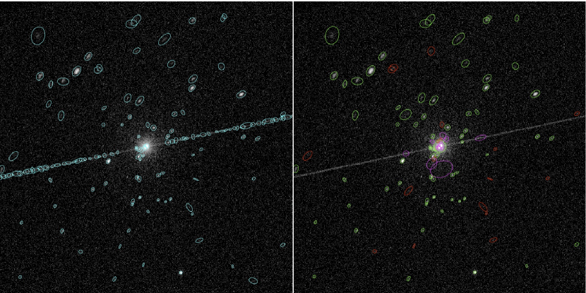
Figure 12.— ACIS broad-band image of the central region of the field of observation 00735 (M81), which includes an extremely bright source that produces a very bright readout streak. Because photon pile-up has eroded the central peak of the bright source, the source is detected incorrectly as multiple close sources that must be rejected manually. Left: Numerous false sources are detected along the length of the readout streak if the latter is not modeled as part of the background. Source detections are shown in cyan. No quality assurance processing has been applied to these detections. Right: When the background map described in the text is used, the false sources are suppressed. Source detections in green are included in the catalog; sources in red do not meet the minimum flux significance criteria for inclusion in the catalog; sources in magenta have been rejected manually during quality assurance processing.

For the algorithm to obtain a good measure of the background, of order 100 bright-source-free rows are required. This condition is satisfied for most observations. Observations with too few source-free rows poorly sample the background. This can lead to erroneously low intensities for bright readout streaks in the resulting background map, which may enhance the false source rate along these streaks. Faint sources that fall in the source-free rows will be considered to be part of the background, which can lead to similar results. Nevertheless, the algorithm is remarkably effective, even in crowded regions such as the Orion complex and the Galactic center fields. An example broad-band ACIS streak map, created for observation 00735 (catalog ADS/Sa.CXO#obs/00735) (M81), is shown in Figure 11, Left.

3.3.2 Low Spatial Frequency Background

For each observation, a low spatial frequency background map is constructed separately for each energy band and image blocking factor (see § 3.4). McCollough & Rots (2008) provide an initial discussion of this algorithm and general background map creation.

As described above, for ACIS observations the high spatial frequency background map includes a component that represents the one-dimensional average of the low frequency background over the rows used to create the streak map. This component, as well as the high spatial frequency background, are removed by subtracting the streak map from the original image from which it was created. For each image blocking factor, the difference image is constructed by subtracting the appropriately regridded streak map from the corresponding blocked original image.

For each pixel in the resulting difference image, a centered sampling region with dimensions $n\times n$ pixels is defined. Spatial scales smaller than $\sim\!n$ pixels are attenuated. The sampling regions are truncated at the edges of the images, and so some higher frequency information may propagate into the background map. However this effect has not been found to have any significant impact on the utility of the resulting map.

A histogram of the count distribution is constructed from the pixels included in the sampling region associated with each image pixel. The first histogram bin will typically span the count range from $-0.5$ to $+0.5$ for ACIS observations, since the readout streak map has been subtracted and there will be some negative pixels. The low spatial frequency background at this image pixel location is computed using a modified form of a Poisson mean

$$b_{\rm lf}=\mbox{\rm mean}[h(a)\cup h(b)\cup h(c)],$$

where $h(x)$ is the number of counts in histogram bin $x$, $a$ is the bin with the maximum number of histogram counts, and $b$ and $c$ are the lower and higher bins immediately adjacent to $a$. The low spatial frequency background map is formed by computing $b_{\rm lf}$ for each pixel location in the image. For ACIS observations, $n=129$ pixels, corresponding to a spatial scale of order $1^{\prime}$ for images blocked at single pixel resolution. Figure 11, Right displays the ACIS broad-band low spatial frequency map for observation 00735 (M81) that corresponds to the streak map shown in the left hand panel of the figure.

3.3.3 Total Background Map

The first step in creating the total background map is to correct the readout streak map (for ACIS observations only) for the effects of reduced exposure near the edges of the observation that arise due to the spacecraft dither, by dividing by the appropriate band-specific normalized exposure map. Similarly, the low spatial frequency background map is corrected by dividing by the smoothed, band-specific normalized exposure map. The smoothing that is applied to the normalized exposure map in the latter case matches the smoothing applied when constructing the low spatial frequency background map. Finally, the two background components for each energy band are summed to produce the total exposure-normalized background map that is required for source detection.

Figure 12 displays the central region of the broad-band ACIS image of M81 (observation 00735), with source detections overlayed. The source detections shown in the left-hand panel are those that result if the background is modeled internally by wavdetect (see § 3.4, below); the panel on the right shows the source detections resulting from using the total background from Fig. 11. Using the background map has eliminated the false sources detected on the readout streak.

The total background maps for each energy band are also archived and accessible through the catalog. These maps differ from those used for source detection in that they have been multiplied by the normalized band-specific exposure map, and are therefore recorded in units of counts. For the convenience of the user, we also store multi-resolution photon-flux images for the full field of each observation, created by filtering the photon event list by energy band, binning to the appropriate image resolution, subtracting the total background map appropriate to the energy band, and dividing by the corresponding exposure map.

3.4. Source Detection

Candidate sources for inclusion in the CSC are identified using the CIAO wavdetect wavelet-based source detection algorithm (Freeman et al., 2002). wavdetect has been used successfully with Chandra data by a number of authors (e.g., Brandt et al., 2001; Giaconni et al., 2002; Lehmer et al., 2005; Kim et al., 2007; Muno et al., 2009), and its capabilities and limitations are well known (e.g., Valtchanov et al., 2001).

Early in the catalog processing pipeline development cycle, several different methods for detecting sources were evaluated. In addition to wavdetect, these included the CIAO implementations of the sliding cell (Harnden et al., 1984; Calderwood et al., 2001) and Voronoi tessellation and percolation (Ebeling & Wiedenmann, 1993) algorithms, and a version of the SExtractor package (Bertin & Arnouts, 1996) modified locally to use Poisson errors in the low count regime.

The Voronoi tessellation and percolation algorithm was quickly discarded because of the significant computational requirements and complexities for automated use. A series of simulations was used to compare the performance of the remaining methods with respect to source detection efficiency for isolated point sources, the efficiency with which close, equally-bright pairs of point sources with $2^{\prime\prime}$ and $4^{\prime\prime}$ separations are resolved, and false source detection rate (A. Dobrzycki, private communication; Hain et al., 2004). The first two properties were evaluated for point sources containing 10, 30, 100, and 2000 counts, with off-axis angles 0–$10^{\prime}$ with $1^{\prime}$ spacing, and nominal background rates for exposure times of 3, 10, 30, and $100\rm\,ks$. The false source rate was evaluated as a function of off-axis angle for the same exposure times.

All three detection algorithms performed reliably for bright, isolated sources located close to the optical axis. Compared to the remaining methods, wavdetect had better source detection efficiency for faint sources located several arcminutes off-axis, and was able to resolve close pairs of sources more reliably than the sliding cell technique. The locally modified version of SExtractor provided inconsistent results, in some cases detecting large numbers of spurious sources.

These simulations were performed early in the catalog processing pipeline development cycle, as an aid in selecting the source detection algorithm to be used for catalog construction. They did not make use of the background maps described in the previous section. The actual performance of the source detection process used to construct the CSC is established from more detailed and robust simulations, as described in § 4 and references therein.

Based on the results of the simulations, wavdetect was selected as the source detection method of choice for the CSC.

The wavdetect algorithm does not require a uniform PSF over the field of view, and is effective in detecting compact sources in moderately crowded fields with variable exposure and Poisson background statistics. To detect candidate sources in a two-dimensional image $D$, wavdetect repeatedly constructs the two-dimensional correlation integral

$$C(x,y;{\bm{\alpha}})=\int\!\int dx^{\prime}\,dy^{\prime}\,W(x-x^{\prime},y-y^{\prime};{\bm{\alpha}})\,D(x^{\prime},y^{\prime})$$ (2)

for a set of Marr (“Mexican Hat”) wavelet functions, $W$, with scale sizes that are appropriate to the source dimensions to be detected. The elliptical form of the Marr wavelet may be written in the dimensionless form

$$W(x,y;{\bm{\alpha}})=(2-\rho^{2})\exp(-\rho^{2}/2),$$ (3)

where

$$\rho^{2}=\frac{1}{a_{1}^{2}}(x\cos\phi+y\sin\phi)^{2}+\frac{1}{a_{2}^{2}}(-x\sin\phi+y\cos\phi)^{2}$$

and the parameters ${\bm{\alpha}}=(a_{1},a_{2},\phi)$ define the semi-major and semi-minor radii and rotation angle of the Mexican Hat.

A localized clump of counts in the image $D$ will produce a local maximum of $C$ if the scale sizes defined by ${\bm{\alpha}}$ are approximately the same as, or larger than, the dimension of the clump. To determine whether a local maximum of $C$ is due to the presence of a source, the detection significance, $S_{i,j}$, in each image pixel $(i,j)$ is determined from

$$S_{i,j}=\int_{C_{i,j}}^{\infty}dC\,p(C|n_{B,i,j}),$$

where $n_{B,i,j}$ is the number of background counts within the limited spatial extent of $W$, and $p(C|n_{B,i,j})$ is the probability of $C$ given the background $B$. If $S_{i,j}\leq S_{0}$, where $S_{0}$ is a defined limiting significance level, then pixel $(i,j)$ is identified as a source pixel.

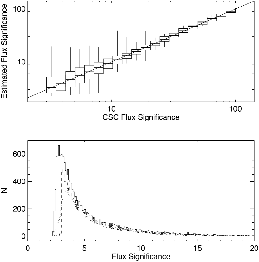
Figure 13.— Top: Estimated flux significance versus catalog flux significance for $\sim\!11,000$ sources detected in the ACIS broad energy band in a pre-release test version of the CSC. The “estimated” flux significance is defined as the ratio ${\tt net\_counts}/{\tt net\_counts\_err}$, as reported by wavdetect, and correlates well with the actual flux significance used the determine catalog inclusion. Horizontal lines indicate the median of the points in each bin, and the vertical lines identify the extreme points. Boxes include 90% of the points in each bin. Bottom: Distribution of estimated flux significances for all detected sources (solid line), including those which fell below the flux significance threshold for the test catalog. The distribution of estimated significances for sources included in the catalog is shown by the dotted line; the dashed line is the distribution of actual flux significances for the same sources. The flux significances for all detected sources extends well below the distributions for sources included in the catalog.

The limiting significance level used to generate the CSC is set to $S_{0}=2.5\times 10^{-7}$. This formally corresponds to $\sim\!1$ false source due to random fluctuations per $2048\times 2048$ pixel image, although due to the heuristics of the algorithm, the actual number of false sources may be lower. The situation is further complicated in our case because the final candidate source list output from the CSC source detection pipeline is a combination of several wavdetect runs in different energy bands (see below). We note that reliable quantitative estimates of the false source rates and detection efficiency can only be provided through simulations, as discussed in § 4. As described in § 2.5, we impose an additional restriction on the flux significance of a source. To ensure that the flux significance requirement is the defining criterion for a source to be included in the catalog, we have verified that the flux significances of sources that pass our wavdetect threshold extend well below that required to satisfy the flux significance rule (see Figure 13). We estimate that roughly $\sim\!1/3$ of all the sources detected by wavdetect fall below this threshold.

Source detection is performed recursively by applying wavdetect to multiply-blocked sky images constructed as described in § 2.5.3. The use of a constant blocked image size maintains algorithm efficiency while not compromising detection efficiency in the outer areas of the field of view where the PSF size is significantly larger than a single pixel.

Applied to the CSC, wavelets with scales $a_{i}=1$, $2$, $4$, $8$, and $16$ (blocked) pixels are computed for each image blocking factor and each energy band except for the ACIS ultra-soft band. This combination of wavelet scales and image blocking factors provides good sensitivity for detection of sources with observed angular extents $\lesssim 30^{\prime\prime}$. Some point sources with extreme off-axis angles, $\theta>20^{\prime}$, may not be detected because the size of the local PSF exceeds the largest wavelet scale/blocking factor combination. F. A. Primini et al. (2010, in preparation) calibrate this effect statistically.

Source detection is not performed in the ACIS ultra-soft energy band. This band is impacted heavily both by increased background and by decreased effective area because of ACIS focal plane contamination (the ratio of integrated background to effective area is 1–2 orders of magnitude larger for the u band when compared to the other ACIS energy bands). Under these circumstances we are limited by the accuracy of the background map determination; small errors in the background map result in an unacceptable fraction of spurious source detections.

The wavdetect algorithm incorporates steps to compare nearby correlation maxima identified at multiple wavelet scales to ensure that each source is counted only once. After duplicates are eliminated, a source cell that includes the pixels containing the majority of the source flux is constructed. Although a source cell may have an arbitrary shape, for simplicity an elliptical representation of the source region is used throughout the CSC. The lengths of the semi-axes of this source region ellipse are set equal to the $3\,\sigma$ orthogonal deviations of the distribution of the counts in the source cell.

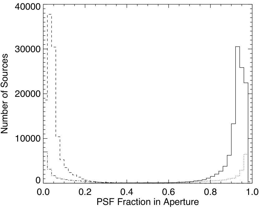
Figure 14.— Histogram of detected source PSF fractions. For sources with off-axis angles $\theta\leq 10^{\prime}$, the PSF fraction included in the source region aperture is shown by the solid line, while the dashed line displays the PSF fraction included in the background region aperture. For sources with $\theta>10^{\prime}$, the dotted line represents the PSF fraction included in the source region aperture and the dash-dotted line indicates the PSF fraction included in the background region aperture.

Source region ellipses for candidate sources detected within a single observation from images with different blocking factors or in different energy bands are combined outside of wavdetect to produce a single merged source list. This step rejects any detections that have RMS radii smaller than the 50% enclosed counts fraction radius of the local PSF, calculated at the monochromatic effective energy of the band in which the source is detected. Such detections are likely artifacts arising from cosmic ray impacts. Candidate source detections whose centroids are closer than the local PSF radius, or that are closer than $3/4$ of the mean detected source ellipse radii, are deemed to be duplicates. If any duplicates are identified, then the detection from the image with the smallest blocking factor is kept, and if the image blocking factors are equal, then the detection with the highest significance is used. This approach ensures that data from the highest spatial resolution blocked image will be used to detect point and compact sources. However, knotty emission that is located on top of extended structures will tend to be identified as distinct compact sources, while the extended emission is not recorded.

3.4.1 Source Apertures

Numerous source-specific catalog properties are evaluated within defined apertures. We define the “PSF 90% ECF (enclosed counts fraction) aperture” for each source to be the ellipse that encloses 90% of the total counts in a model PSF centered on the source position. Because the size of the PSF is energy dependent, the dimensions of the PSF 90% ECF aperture vary with energy band.

We define the “source region aperture” for each source to be equal to the corresponding $3\,\sigma$ source region ellipse included in the merged source list, scaled by a factor of $1.5\times$. Like the PSF 90% ECF aperture, the source region aperture is also centered on the source position, but the dimensions of the aperture are independent of energy band. Evaluation of model PSFs with off-axis angles $\lesssim 10^{\prime}$ demonstrates that the dimensions of the source region aperture correspond approximately to the dimensions of the PSF 90% ECF ellipses for the ACIS broad energy band. This is confirmed a posteriori by examining the distribution of PSF aperture fractions in source and background (see below) region apertures of all individual catalog sources with ACIS broad band flux significance ${}\geq 3.0$. Figure 14 demonstrates that the source region apertures typically include $\sim\!90$–95% of the PSF, while the background region apertures contain $\lesssim 5$–10%. We emphasize that while these fractions are typical, the actual PSF fractions, determined by integrating the model PSF over the source and background region apertures and excluding regions from contaminating sources, are used for the actual determination of source fluxes (see § 3.7).

Comparison of the source fluxes within the PSF 90% ECF aperture and the source region aperture provide a crude indication whether a source is extended. If the flux in the source region aperture is significantly greater than the flux in the PSF 90% ECF aperture, then the source region determined by wavdetect is considerably larger than the local PSF, and the source is likely extended.

Both the PSF 90% ECF aperture and the source region aperture are surrounded by corresponding background region annular apertures. In both cases, the inner edge of the annulus is set equal to the outer edge of the corresponding source aperture, while the radius of the outer edge of the annulus is set equal to $5\times$ the inner radius of the source region aperture. Although the background region apertures defined in this manner include $\sim\!5$–10% of the X-rays from the source, this contamination is accounted for explicitly when computing aperture photometry fluxes.

Overlapping sources could contaminate any measurements obtained through the source and background apertures. To avoid this, both types of apertures are modified to exclude areas that are included in any overlapping source region apertures, or that fall off the detector. Areas surrounding ACIS readout streaks are also excluded from the modified background apertures. Aperture-specific catalog quantities are derived from the event data in the appropriate modified aperture. The fractions of the local model PSF counts that are included in the modified apertures are recorded in the catalog for each source, and are used to apply aperture corrections when computing fluxes, under the assumption that the source is well modeled by the PSF.

The modified source region and background region aperture definitions are recorded as FITS files using the spatial region file convention (Rots & McDowell, 2008). CIAO (Fruscione et al., 2006) can be used to apply these regions as spatial filters to extract the photon event data for the source (or background) from the archived photon event list. To simplify access to file-based data products (see Table 3) for individual sources, we also separately store the source region photon event list, per-band exposure maps, and per-band source region images. These products include data from the rectangular region of the sky that is oriented North–South/East–West and that bounds the background region.

3.4.2 Matching Source Detections from Multiple Observations

Each source record in the CSC Master Sources Table is constructed by combining source detections included in the Source Observations Table from one or more observations. A necessary first step in this process requires matching the source detections from all of the observations that include the same region of the sky. Cross-matching algorithms (e.g., Devereux et al., 2005; Gray et al., 2006) are often focussed on efficiently matching large catalogs, and typically use criteria on the position difference distribution, or cross-correlation approach techniques, for identifying matches. In many cases, these approaches assume (often implicitly) that the source PSF is at least approximately spatially uniform across the field of view, and comparable between the datasets being matched.

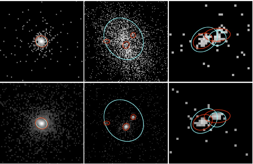
Figure 15.— Left: Upper and lower images illustrate the common source matching case where the source detections from the individual observations all uniquely match a single source on the sky. The source region aperture determined from the upper image is shown in cyan, while the source region aperture determined from the lower image is shown in red. Center: In this case, the off-axis source region aperture computed from the source detection in the upper image, shown in cyan, overlaps multiple source region apertures from the observation in the lower image, shown in red. The cyan source detection is confused, and will be connected to the master sources associated with the red source detections using “ambiguous” linkages. Right: The sources detected in these observations for a confused “pair of pairs.” The fractional overlaps between the pair of cyan source region apertures and the pair of red source region apertures is sufficiently large that these detections are assigned to be resolved by human review.

However, when matching source detections across multiple Chandra observations, the strong dependence of the PSF size with off-axis angle must be considered explicitly, since source detections that are well off-axis in one observation are often resolved into multiple sources close to the optical axis in other observations. Under these circumstances the source positions determined by wavdetect are not comparable, and cannot be used for source matching. Instead, the source matching approach used for the CSC is based on the overlaps between the PSF 90% ECF apertures of the source detections from the individual observations. Although empirical in nature, this algorithm works well for matching compact source detections between Chandra observations.

The detailed algorithm is described in Appendix A. The method identifies the overlap fractions between the PSF 90% ECF apertures of overlapping source detections from the observations, and separates them into three different categories.

The first category is the simplest, where the source detections from the various observations have apertures that all mutually overlap (Fig. 15, Left). This is the most common situation, and corresponds to the case where the source detections all uniquely match a single source on the sky. Roughly 90% of the $\sim\!18,000$ sources in the Master Sources Table that are linked to more than one source detection in the Source Observations Table fall into this category. Each of the matching entries in the latter table will be associated with the corresponding Master Sources Table entry with a “unique” linkage, as described in § 2.3.

In the second category, the aperture associated with a source detection in one observation overlaps the apertures associated with multiple distinct source detections from other observations. This circumstance typically arises because source detections from a single observation are always assumed to be distinct; this assumption can fail very far off-axis ($\theta\gtrsim 20^{\prime}$), where the PSF size exceeds the maximum wavdetect wavelet scale/image blocking factor combination. This category is illustrated in Figure 15, Center, and arises most often because a source detection in one observation is resolved into multiple sources by one or more of the overlapping observations. The unresolved source detection in the Source Observations Table will be connected to all Master Sources Table entries associated with the matching resolved source detections via “ambiguous” linkages, and the detection will be flagged as confused. The X-ray photon events associated with the unresolved detection cannot be distributed across the matching resolved sources. In release 1 of the CSC, source properties derived from the detection will not be used to compute the source properties included in the Master Sources Table. Upper limits for photometric quantities could in principle be extracted from the unresolved source detection, and these would be quite valuable for variability studies. This capability will be included in a future release of the CSC.

In a few cases, a set of aperture overlaps cannot be resolved automatically using the current algorithm. This third category typically occurs when there are multiple overlapping, confused source detections. In this case, the source detections are flagged for review by a human, who is then responsible for resolving the matches. Only 415 (out of 94,676) master sources include source detections that required manual review, and the majority of these were readily resolved as confused “pairs of pairs.” The latter case, which is illustrated in Figure 15, Right commonly occurs because a pair of source detections included in a single observation both overlap a pair of source detections in another observation. Each of the source detections in the first observation overlaps both source detections in the second observation, making the detections confused, and vice-versa. If a manual review is required to complete a match for a specific source, then a flag is set in the catalog to indicate this fact.

The actual processing required to perform the matches is complex. Whenever new overlapping source detections are identified during catalog processing, the set of matches is recomputed using all of the observations processed so far. The algorithm then queries the prior state of the catalog, and determines the set of updates that are necessary to migrate from that state to the newly determined state. This procedure works regardless of the order in which observations processed, and also permits an already-processed observation to be reprocessed should an error have occurred.

3.4.3 Source Naming

Each distinct X-ray source included in the Master Sources Table is assigned a name that is derived from the source’s location on the sky. Catalog sources are designated “CXO J$\hbox{\it HHMMSS.s\/}\pm\hbox{\it DDMMSS\/}$,” where HHMMSS.s and $\pm\hbox{\it DDMMSS\/}$ are the ICRS right ascension and declination, respectively, of the source position, truncated to the indicated precision. This format complies with the International Astronomical Union (IAU) Recommendations for Nomenclature. The “CXO” prefix is registered with Commission 5 of the IAU for exclusive use in source designations issued by the Chandra X-ray Center.

The name assigned to a source is determined from the combined source position once the detections of the source are merged according to § 3.4.2. If the source has never been included in a released version of the CSC, then the source name may be revised if a source detection in a subsequently processed observation modifies the combined source position. Therefore, the name assigned to a source that is visible in a database view may change as new observations are processed, if the source has never been included in a catalog release.

Once a source is included in a released version of the CSC, then the name of that source is frozen. The name will not be changed in either future catalog release views (i.e., subsequent catalog releases) or database views, even if additional observations refine the source position. Therefore minor discrepancies can arise between the latter and the source designation. However, if an observation included in a later catalog release resolves an apparently single source included in an earlier version of the catalog into multiple distinct sources, then the previous source designation is retired and new names are assigned to the resolved sources.

3.5. Source Position Determination

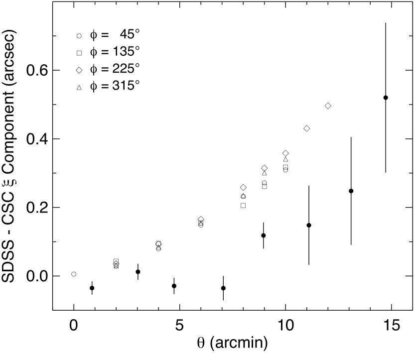
Figure 16.— Mean (signed) coordinate differences between SDSS and CSC source positions measured along the ${\bm{\xi}}$ vector (defined in the text) as a function of off-axis angle, $\theta$, for individual observations of CSC sources with at least 500 net counts are shown as filled circles. Open symbols indicate expected values computed from high SNR ray-trace simulations at the indicated values of $\theta$ and $\phi$. Note that the measured mean coordinate differences are consistent with zero offset for $\theta\lesssim 8^{\prime}$, and are a factor $\sim\!2$ times smaller than the model predictions for larger values of $\theta$.

Within a single observation, the detected source positions are those assigned by the wavdetect algorithm. Their accuracy can be estimated by evaluating the mean (signed) coordinate differences between the wavdetect positions and the positions of matching sources in the seventh data release (DR7) of the Sloan Digital Sky Survey (SDSS; Abazajian et al., 2009). The latter are extracted from the CSC/SDSS Cross-Match Catalog. As shown in Figure 16, the mean coordinate differences demonstrate good position agreement between the CSC and SDSS for sources with $\theta\lesssim 8^{\prime}$ (where we have restricted the comparison to include only individual observations of CSC sources with at least 500 net counts to minimize statistical errors).

For larger off-axis angles, Figure 16 suggests that there may be a systematic offset between the wavdetect source positions and the SDSS source positions. The measured mean position difference is $\lesssim 0\farcs 3$ for $\theta\lesssim 15^{\prime}$, but appears to increase with off-axis angle. The exact cause of this offset is uncertain. Some authors (e.g., Alexander et al., 2003; Lehmer et al., 2005; Luo et al., 2008) have reported a similar effect, which they attribute to centroiding errors introduced by of the asymmetric nature of the Chandra PSF at large off-axis angles.

High quality PSF simulations generated using the SAOTrace (formerly SAOsac) ray-trace code (Jerius et al., 1995, 2004) confirm that the asymmetry can displace the measured centroid from the requested location of the simulated PSF on a uniform pixel grid. We designate the vector orientation from the measured centroid position to the requested location of the PSF as ${\bm{\xi}}$. As shown in Figure 16, the expected centroid displacement along ${\bm{\xi}}$ computed from the simulations is not a good measure of the actual mean coordinate difference, which is a factor of order 2 times smaller than predicted by the models. One possible reason for the disagreement between the model and actual measurements is that the Chandra plate scale calibration was derived from observations of NGC 2516 and LMC X-1 using source centroid measurements that were not corrected for the asymmetry of the PSF (Markevitch, 2001b).

As described in § 2.5.3, the celestial coordinates of a source observed by Chandra are computed by applying a series of transforms to the measured position of the source on the detector. The final step in this process applies the measured plate scale calibration to the difference between the position of the source on the virtual sky pixel plane and a known fiducial point, which is typically the telescope optical axis. If all of the star-star baselines used to calibrate the plate scale were oriented parallel to ${\bm{\xi}}$, then the lack of correction for the PSF asymmetry would to first order compensate for the linear component of the systematic position offset when measuring real sources whose locations are fixed in world coordinates rather than virtual pixel plane coordinates. Since not all star-star baselines were so aligned, some residual systematic position offset may be expected, but at an undetermined level that is less than predicted from the PSF simulations.

Systematic position offsets can also arise from uncertainties in the detector geometry. As an example, consider imaging observations that use the nominal ACIS-I aimpoint. Sources with $\theta\lesssim 8^{\prime}$ will be located on the same CCD array as the aimpoint. As $\theta$ increases, an increasing fractions of sources will instead be positioned on ACIS-S array CCDs, until for $\theta\gtrsim 11^{\prime}$ all sources will be located on the ACIS-S array. Uncertainties in the relative positions and tilts of the ACIS-I and ACIS-S arrays would therefore introduce systematic position offsets for sources with large off-axis angles, while not impacting sources that fall on the same CCD array as the aimpoint. This signature is consistent with the absence of mean position differences measured for $\theta\lesssim 8^{\prime}$.

Because of the small magnitude of the mean position differences measured for $\theta\lesssim 15^{\prime}$, we have chosen not to apply an uncertain correction to source positions in release 1 of the catalog. We plan to investigate in detail the cause of the systematic position offsets at large off-axis angles, and adjust source positions in future catalog releases if appropriate.

3.5.1 Source Position Uncertainty

In addition to reporting measured source positions, wavdetect also reports positional errors associated with each source detection. The reported errors are based on a statistical moments analysis, and do not consider instrumental effects such as pixelization, aspect-induced blur, or asymmetrical PSF structure that may contribute to the total positional uncertainties. Simulations that compare the reference positions of artificially generated sources with their positions determined by wavdetect indicate that the positional uncertainties computed by wavdetect are underestimated for sources with large off-axis angles. The simulation results, which quantify the dependence of positional uncertainties of simulated sources on off-axis angle, were found to be consistent with the more extensive simulations uses to construct the Chandra Multiwavelength Project (ChaMP) X-ray point source catalog (Kim et al., 2007).

In the first release of the CSC, source position error ellipses are substituted by error circles computed using the ChaMP positional uncertainty relations

$$\log P=\left\{\begin{array}[]{l}0.1145\theta-0.4957\log S_{w}+0.1932\\ \quad\quad\quad\quad\quad\quad 0.0000<\log S_{w}\leq 2.1393\\ 0.0968\theta-0.2064\log S_{w}-0.4260\\ \quad\quad\quad\quad\quad\quad 2.1393<\log S_{w}\leq 3.3000.\end{array}\right.$$ (4)

In these equations, $P$ is the positional uncertainty in arcseconds, $\theta$ is the off-axis angle in arcminutes, and $S_{w}$ is the source net counts reported by wavdetect. These relations were derived to characterize the positional uncertainties at the 95% confidence level of X-ray point sources in the ChaMP X-ray point source catalog, which includes $\sim\!6,800$ X-ray sources detected in 149 Chandra observations. The values of $\log P$ computed using equations (4) are not equal at the boundary where $\log S_{w}=2.1393$ (roughly 138 net counts). However, this error is negligible for $\theta\lesssim\!10^{\prime}$.

Although HRC observations are not included in the first release of the CSC, we have used a series of simulations to derive an improved positional uncertainty relation that is appropriate for sources detected in HRC-I observations. The simulations include $\sim\!6,000$ point sources spanning $0<\theta<22^{\prime}$ and $9<S_{w}<3600$. The best fit surface for the 95% position uncertainty quantile is

$$\log P = 0.752569+0.216985\theta+0.000242\theta^{2}$$

$$-1.142476\log S_{w}+0.172132\log^{2}S_{w}$$

$$-0.040549\theta\log S_{w}.$$

The simulations do not sample the region with $\theta>20^{\prime}$ and $S_{w}<\sim\!50$, and so we impose an upper bound of $\log P=2.128393$ on this relation, to cap the uncertainty in this regime.

In release 1.1 of the CSC, positional uncertainties for sources detected in ACIS observations are computed using equation (4) while positional uncertainties for sources detected in HRC-I observations are computed using equation (3.5.1).

The positional uncertainties from equations (4) and (3.5.1) provide a good measure of the statistical uncertainty of the location of the source in the frame of the observation, but do not consider potential sources of error that are external to the observation. These include the error in the mean aspect solution for the observation, the astrometric errors in the AXAF (Chandra) Guide and Acquisition Star Catalog (Schmidt & Green, 2003), and the calibration of the geometry of the spacecraft and focal plane. As described in § 4.3, Rots (2009) has recently used the CSC/SDSS Cross-Match Catalog to calibrate the combined external error by analyzing the statistical distribution of the measured separations of CSC point source detections from individual observations with their counterparts in SDSS DR7 (Abazajian et al., 2009).

The resulting external astrometric error is $0\farcs 16\pm 0\farcs 0.01$ ($1\,\sigma$), or $0\farcs 39$ (95% confidence). The latter must be added in quadrature to the position uncertainties from equations (4) and (3.5.1) to compute the absolute position error for CSC sources. In release 1 of the catalog, the positional error reported in the catalog tables is taken directly from equation (4), so the quadrature addition of the external astrometric error component must be performed by the user. Release 1.1 of the CSC will include this error component directly in the tabulated values.

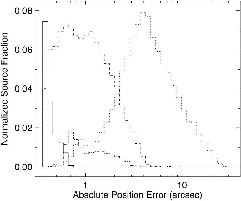
Figure 17.— Histograms of the total absolute position error for source detections included in release 1 of the CSC. The dashed and dotted lines include all source detections with off-axis angles $\theta<8^{\prime}$ and $8^{\prime}\leq\theta<15^{\prime}$, respectively. Each histogram is normalized by the total number of source detections within the relevant $\theta$ range. Source detections with at least 500 net counts are shown with the solid line ($\theta<8^{\prime}$) and dash-dotted line ($8^{\prime}\leq\theta<15^{\prime}$). For the latter two histograms, the normalized source fraction has been scaled by a factor of $4\times$.

A post facto histogram of the 95% confidence positional uncertainties, including the external astrometric error, for source detections included in release 1 of the CSC is presented in Figure 17. The figure demonstrates that statistical errors due to lack of net source counts does dominate the positional uncertainty for all but the brightest sources. However, for bright sources detected at small off-axis angles, the external astrometric error limits the accuracy of the derived source positions. Any error introduced by using uncorrected source centroid positions from wavdetect is negligible for the overwhelming majority of source detections.

3.5.2 Combining Source Positions from Multiple Observations

Improved estimates of the position and positional uncertainty of each X-ray source are determined from the statistically independent source detections included in the set of individual observations using a multivariate optimal weighting formalism. This technique is effective in cases where simple averaging fails, for example when the area defining the source position varies significantly from observation to observation. We express the uncertainties of the estimates in the form of error ellipses centered upon the estimated source positions. An equivalent approach has been used for weapons targeting (Orechovesky, 1996). To our knowledge the usage here is the first documented application to astrophysical data.

In the multivariate optimal weighting formalism, given a set of estimates, $X_{i}$, of the mean of some two-dimensional quantity, and the $2\times 2$ covariance matrices, $\sigma_{i}^{2}$, associated with these estimates, an improved estimate, $X$, of the mean, and the associated covariance matrix, $\sigma^{2}$, are (e.g., Davis, 2007b)

$$X=\sigma^{2}\sum_{i}\frac{X_{i}}{\sigma_{i}^{2}} ;\quad \sigma^{2}=\left[\sum_{i}\frac{1}{\sigma_{i}^{2}}\right]^{-1}.$$ (6)

For the application described here, we take $X_{i}$ to be the $i$th estimate of the source position, projected onto a common tangent plane (which is constructed at the mean position of the ellipse centers). The corresponding covariance matrix is

$$\begin{array}[]{l}\!\!\sigma_{i}^{2}=\\ \;\left(\begin{array}[]{cc}\sigma^{\prime 2}_{1,i}\cos^{2}\vartheta_{i}+\sigma^{\prime 2}_{2,i}\sin^{2}\vartheta_{i}&(\sigma^{\prime 2}_{2,i}-\sigma^{\prime 2}_{1,i})\cos\vartheta_{i}\sin\vartheta_{i}\\ (\sigma^{\prime 2}_{2,i}-\sigma^{\prime 2}_{1,i})\cos\vartheta_{i}\sin\vartheta_{i}&\sigma^{\prime 2}_{1,i}\sin^{2}\vartheta_{i}+\sigma^{\prime 2}_{2,i}\cos^{2}\vartheta_{i}\end{array}\right),\end{array}$$

where $\sigma^{\prime}_{1,i}$ and $\sigma^{\prime}_{2,i}$ are the lengths of the semi-minor and semi-major axes, respectively, of the $i$th error ellipse projected onto the common tangent plane, and $\vartheta_{i}$ is the angle that the major axis of the $i$th error ellipse makes with respect to the tangent plane $y$ axis. The derivation of equation (3.5.2) is presented in Appendix B.

Once the covariance matrices corresponding to the error ellipses for each individual source observation, equation (3.5.2), are computed, the error ellipses are combined using equation (6). This yields the optimally weighted source position and position error ellipse for the combined set of observations, on the common tangent plane. Mapping these back to the celestial sphere provides the combined source position and error ellipse estimates.

3.6. Source Extent Estimates

The observed spatial extent of a source is estimated using a rotated elliptical Gaussian parameterization of the form

$$S(x,y;\alpha)=\frac{s_{0}}{\sigma_{1}\sigma_{2}}\exp\left[-\pi(\mathcal{A}\mathbf{x})^{2}\right],$$ (7)

where

$$\mathcal{A}=\left({\begin{array}[]{cc}\sigma_{1}^{-1}&0\\ 0&\sigma_{2}^{-1}\end{array}}\right)\left({\begin{array}[]{cc}\cos\phi_{0}&\sin\phi_{0}\\ -\sin\phi_{0}&\cos\phi_{0}\end{array}}\right) ;\quad \mathbf{x}=\left({\begin{array}[]{cc}x\\ y\end{array}}\right),$$

where $(x,y)$ is the Cartesian center location of the Gaussian, and the parameters $\alpha=(\sigma_{1},\sigma_{2},\phi_{0})$ are the $1\,\sigma$ radii along the major and minor ellipse axes, and the position angle of the major axis of the ellipse, respectively.

The parameters of $S$ are determined using a wavelet-based approach that is similar to that used for source detection. The methods differ in their details and assumptions, however.

For source detection, the choice of wavelet scales used by wavdetect to detect sources is determined a priori. Because of the strong variation of PSF size with off-axis angle, multiple wavelet scales and input image blocking factors are required to search for sources at all off-axis angles, as described in § 3.4. Stepping between the discrete wavelet scales and image blocking factors as a function of off-axis angle introduces small but systematic biases in the derived dimensions of the source region ellipses (and therefore the source region apertures; see Figure 18).

Photometric, spectral, and temporal properties determined from the X-ray events included in the aperture are not impacted by these effects, since the aperture dimensions are sufficiently large that they typically enclose $\sim\!90\%$ of the PSF counts, and a correction factor is applied for the fraction of the PSF that falls outside of the aperture. However, these biases render the source region aperture dimensions unsuitable for use as a measure of the source extent.

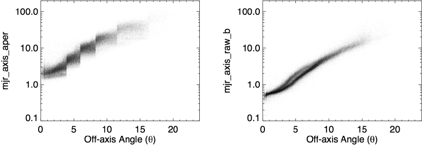
Figure 18.— Comparison of source region aperture dimensions with raw (undeconvolved) source extent for the ACIS broad (b) energy band for all source observations included in the first release of the CSC. Left: Semi-major axis of the source region aperture is plotted for each source observation versus source off-axis angle, $\theta$. The step-like structure visible in the plot results from the stepping between discrete wavelet scales and image blocking factors as a function of off-axis angle. Right: Semi-major axis of the raw (undeconvolved) ACIS broad (b) energy band source extent is plotted versus $\theta$. The source extent is derived using a scaleless wavelet approach, as described in the text, and varies smoothly with $\theta$. Differing geometric tilts of the ACIS-I and ACIS-S CCD arrays relative to the focal plane split the distribution into separate populations for $3^{\prime}\lesssim\theta\lesssim 7^{\prime}$. The lower population corresponds to point sources located on ACIS-I array CCDs, while point sources located on ACIS-S array CCDs comprise the upper population. The difference in the vertical scales between the two plot panels results because the source region aperture scales approximately as the PSF 90% ECF, whereas the source extent estimates the $1\,\sigma$ scale of an elliptical Gaussian parameterization of the source.

The wavelet-based approach used for estimating the source extent determines the optimal wavelet scale size directly from the data under the assumption that a source exists at approximately the location determined by wavdetect. The raw source extent estimates derived using this approach vary smoothly with off-axis angle (Fig. 18).

The two-dimensional correlation integral

$$\begin{array}[]{l}\!\!C(x,y;{\bm{\alpha}})=\\ \quad\int_{-X}^{X}\int_{-Y}^{Y}dx^{\prime}\,dy^{\prime}\,W(x-x^{\prime},y-y^{\prime};{\bm{\alpha}})\,S(x^{\prime},y^{\prime};{\bm{\alpha}}),\end{array}$$ (9)

where the region of interest is $|x^{\prime}|\leq X$ and $|y^{\prime}|\leq Y$, and $W$ is again specified by equation (3), is computed first.

We choose a coordinate system in which the peak of $S$ is centered at the origin. The quantity $\psi(x,y;{\bm{\alpha}})=C(x,y;{\bm{\alpha}})/(a_{1}a_{2})^{1/2}$ has a maximum value at the origin when $a_{i}=\sigma_{i}\sqrt{3}$ and $\phi=\phi_{0}$ (Damiani et al., 1997). The source parameters are determined by maximizing $\psi$.

In practice, equation (9) is evaluated as a discrete sum over the pixels of the image. Although integration of equation (3) does not yield a simple closed-form solution, and numerical integration is computationally expensive, for the purpose of optimizing $\psi_{0}=C(0,0;{\bm{\alpha}})/(a_{1}a_{2})^{1/2}$, a rectangular approximation for the integral over each pixel is sufficient. In this approximation,

$$W_{mn}(x_{i},y_{j};{\bm{\alpha}})\approx W(x_{m}-x_{i},y_{n}-y_{j};{\bm{\alpha}})\Delta x\Delta y,$$

where $W(x,y;{\bm{\alpha}})$ is evaluated at the center of each pixel and the pixel area is $\Delta x\Delta y$.

A small sub-image of the source is extracted centered on the source position determined by wavdetect. The accuracy of this source position is refined by searching the center of the sub-image for the coordinates $(x_{0},y_{0})$ that maximize $\psi_{0}(x,y;a,a,0)$. A new sub-image is then extracted using the improved source position.

Finally, the size and orientation of the elliptical Gaussian source parameterization are derived by maximizing $\psi(x_{0},y_{0};{\bm{\alpha}})$. Choosing good initial values for $a_{i}$ helps to ensure that this optimization step converges reliably. We set the initial values $a_{1}=a_{2}=\max{[(d_{1}d_{2})^{1/2},a_{\rm grid}}]$, where $d_{i}$ are the ellipse semi-axes derived by wavdetect, and the value of $a_{\rm grid}$ is obtained by examining $\psi_{0}(x_{0},y_{0};a,a,0)$ on a grid of $a$ values spanning the half-width of the source image; $a_{\rm grid}$ is usually the smallest $a$ that corresponds to either a local maximum or an inflection point. This choice is motivated by the observation that when a single source is present, the location of a local maximum provides a good estimate of the source size (see Figure 19). Similarly, when the source of interest is blended with other nearby sources, an inflection point where $\partial^{2}_{a}\psi_{0}=0$ often occurs near the “edge” of the central source. When the first occurrence of $\partial_{a}\psi_{0}=0$ occurs at a local minimum, $a_{\rm grid}$ is the smallest value of $a$ on the pixel grid.

3.6.1 PSF Extent

The spatial extent of the local PSF is determined for comparison with the observed source extent, and as an aid to assessing the intrinsic extent of the source. Since the size of the Chandra PSF is a strong function of off-axis angle, a ray-trace model is constructed at the measured off-axis and azimuthal angles $(\theta,\phi)$ separately for each detected source. Although the shape of the PSF is energy-dependent, within each energy band the ray-trace model is computed only at the monochromatic effective energy (see § 2.5.2) of the band. This approximation results in an error that is dependent on the actual spectrum of the source, but that does not exceed $\sim\!10\%$ for typical power-law or black-body source spectra.

The ray-trace model is computed using version 1.0.0 of the SAOTrace simulation code (Jerius et al., 1995, 2004) with the latest HRMA optical coefficients derived from calibration observations. A ray density of $\rm 0.2\,\hbox{rays}/\hbox{mm}^{2}$ is used for the ray-trace. The rays are then projected onto the detector focal plane, a Gaussian blur is applied to account for the degradation due to de-dithering the telescope motion ($\sigma=0\farcs 148$ for ACIS, $0\farcs 2$ for HRC), and the image is resampled onto the pixel plane of the detector. Each PSF image is recorded in the CSC as a file-based data product (see Table 3), which can be retrieved by the catalog user and compared directly to the corresponding source region image.

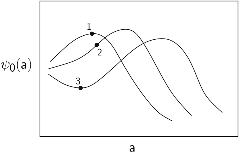
Figure 19.— Deriving a correlation scale length from the shape of $\psi_{0}(a)$. Three curves are shown, schematically illustrating the different shapes that $\psi_{0}(a)$ can have. An unblended source normally yields a distinct local maximum (point 1). Depending on the source spacing, closely spaced sources may yield an inflection point (point 2) or a local minimum (point 3). The text describes how each of these cases is treated.

The ray density used in the ray-trace models typically produces a total of $\sim\!6$–$8\times 10^{3}$ counts (with a full range of $\sim\!4$–$13\times 10^{3}$ counts) in the resulting PSF model in the ACIS broad, hard, and soft energy bands, where the combined HRMA/instrument effective area at the monochromatic effective energies of the bands is $\sim\!300$–$400\rm\,cm^{2}$. The number of counts in the ACIS medium energy band PSF models is about 60% higher, because of the higher effective area at that band’s monochromatic effective energy. For the ACIS ultra-soft energy band the total PSF counts may be only a few hundred because of the poor quantum efficiency in the band. Although the PSF models computed here are sufficient for their intended purposes of providing basic estimates of source extent and point source aperture corrections for aperture photometry, they are not suitable for analyses such as image deconvolution that require detailed PSF models.

Once the image of the local model PSF is constructed, the rotated elliptical Gaussian parameterization, $p(x,y;b_{1},b_{2},\psi)$, of the spatial extent is computed in the same way that the observed source extent, $S(x,y;\sigma_{1},\sigma_{2},\phi_{0})$, is computed from the source image.

3.6.2 Intrinsic Source Extent

Using the rotated elliptical Gaussian parameterizations derived above, the observed source extent, $S(x,y;\sigma_{1},\sigma_{2},\phi_{0})$, can be treated as the convolution of the local PSF, $p(x,y;b_{1},b_{2},\psi)$ with the intrinsic source extent, $s(x,y;a_{1},a_{2},\phi)$, where we parameterize the latter similarly to equation (7). In general, $\phi_{0}\neq\phi$, since the PSF-convolved ellipse need not have the same orientation as the intrinsic source ellipse.

In principle, one can determine the parameters, $(a_{1},a_{2},\phi)$, of the intrinsic source ellipse by solving a nonlinear system of equations involving the PSF parameters, $(b_{1},b_{2},\psi)$, and the observed source parameters, $(\sigma_{1},\sigma_{2},\phi_{0})$. However, because these equations are based on simple assumptions regarding the source and PSF profiles, and because the input parameters are often uncertain, such an elaborate calculation seems unjustified.

A much simpler and more robust approach makes use of the identity

$$\sigma_{1}^{2}+\sigma_{2}^{2}=a_{1}^{2}+a_{2}^{2}+b_{1}^{2}+b_{2}^{2},$$

which applies to the convolution of two elliptical Gaussians having arbitrary relative sizes and position angles. Using this identity, one can define a root-sum-square intrinsic source size,

$$a_{\rm rss} = \frac{1}{\sqrt{2}}\left(a_{1}^{2}+a_{2}^{2}\right)^{1/2}$$ (10)

$$= \frac{1}{\sqrt{2}}\max\left[0,(\sigma_{1}^{2}+\sigma_{2}^{2})-(b_{1}^{2}+b_{2}^{2})\right]^{1/2},$$

that depends only on the sizes of the relevant ellipses and is independent of their orientations. This expression is analogous to the well-known result for convolution of one-dimensional Gaussians and for convolution of circular Gaussians in two dimensions. The factors of $1/\sqrt{2}$ ensure that the statistic value gives the radius of the source image when applied to circular source images.

Using equation (10), one can derive an analytic expression for the uncertainty in $a_{\rm rss}$ in terms of the measurement errors associated with $\sigma_{i}$ and $b_{i}$. Because $\sigma_{i}$ and $b_{i}$ are non-negative, evaluating the right-hand side of equation (10) using the corresponding mean values should give a reasonable estimate of the mean value of $a_{\rm rss}$. A Taylor series expansion of the right-hand side of equation (10) evaluated at the mean parameter values therefore yields the uncertainty

$$\begin{array}[]{l}\!\Delta a_{\rm rss}=\\ \;\frac{1}{\sqrt{2}a}\left[\sigma_{1}^{2}(\Delta\sigma_{1})^{2}+\sigma_{2}^{2}(\Delta\sigma_{2})^{2}+b_{1}^{2}(\Delta b_{1})^{2}+b_{2}^{2}(\Delta b_{2})^{2}\right]^{1/2},\end{array}$$

where $(\Delta X)^{2}$ represents the variance in $X$, and where

$$a=\left\{\begin{array}[]{c l}a_{\rm rss}&\quad a_{\rm rss}>0\\ \sqrt{b_{1}^{2}+b_{2}^{2}}&\quad a_{\rm rss}=0.\end{array}\right.$$

3.6.3 Combining Intrinsic Source Extent Estimates from Multiple Observations

Measurements of the mean intrinsic source extent derived from multiple independent observations, $a_{{\rm rss},i}\pm\Delta a_{{\rm rss},i}$, are combined using the multivariate optimal weighting formalism, equations (6). The minimum variance estimator of the intrinsic source size is the variance-weighted mean,

$$\overline{a_{\rm rss}}={\rm Var}[\overline{a_{\rm rss}}]\sum_{i}{\rm Var}[a_{{\rm rss},i}]^{-1}a_{{\rm rss},i},$$

where ${\rm Var}[a_{{\rm rss},i}]=(\Delta a_{{\rm rss},i})^{2}$. The variance in $\overline{a_{\rm rss}}$ is

$${\rm Var}[a_{\rm rss}]=\left[\sum_{i}{\rm Var}[a_{{\rm rss},i}]^{-1}\right]^{-1}.$$

3.7. Aperture Photometry

Net source counts, count rates, and photon and energy fluxes for point sources are computed from counts and exposure data accumulated in independent source and background apertures, $R_{s}$ and $R_{b}$. Typically, these apertures are simple elliptical regions and surrounding elliptical annuli, but arbitrary areas from either aperture may be excluded to avoid contamination from nearby sources, or missing data due to detector edges. The net aperture areas, $A_{s}$ and $A_{b}$, and the fractions, $\alpha$ and $\beta$, of source counts expected in both apertures are determined from

$$A_{s}=\int_{R_{s}}dxdy ;\quad A_{b}=\int_{R_{b}}dx\,dy$$

and

$$\alpha=\int_{R_{s}}dx\,dy\,\mathit{PSF}(x,y) ;\quad \beta=\int_{R_{b}}dx\,dy\,\mathit{PSF}(x,y).$$

We use the PSFs described in § 3.6.1 to estimate $\alpha$ and $\beta$. Although the finite number of PSF counts leads to some uncertainty in the estimate for $\beta$, the effect of this uncertainty on the derived net counts, count rates, and fluxes is small (typically $\ll 1\%$).

If a uniform background over the scale of $R_{s}$ and $R_{b}$ is assumed, then the net source counts with aperture corrections applied, $S$, can be determined by solving the simultaneous set of linear equations

$$C=\alpha S+b ;\quad B=\beta S+rb,$$ (11)

where $C$ and $B$ are the total counts in $R_{s}$ and $R_{b}$, respectively, $b$ represents the background in $R_{s}$, and $r=A_{b}/A_{s}$. The solution is

$$S=(rC-B)/(r\alpha-\beta).$$

In general, selecting a background aperture so that $\beta\rightarrow 0$ is difficult, since the inner radii of such annuli could range from $\sim\!25^{\prime\prime}$ to $>\!1000^{\prime\prime}$, depending on $\theta$ and energy. Such large background apertures would be subject to errors due to intrinsic background variations, diffuse source emission, and background contributions from multiple detector chips. We choose rather to use smaller apertures, containing $\sim\!5$–10% of the source flux (see Fig. 14), whose effects can be modeled more accurately.

To apply a consistent statistical approach in determining confidence bounds for all photometric quantities (see below), we assume that the generic photometric quantity $S$ (whether counts, count rate, photon flux, or energy flux) can be converted to counts by multiplying by appropriate generic conversion factors $f$ and $g$ defined below, averaged over $R_{s}$, $R_{b}$, and generalize equations (11) to include these terms,

$$C=fS+b ;\quad B=gS+rb.$$ (12)

For example, if $S$ represents a count rate, $f=\alpha\langle T_{s}\rangle$ and $g=\beta\langle T_{b}\rangle$, where $\langle T_{s}\rangle$ and $\langle T_{b}\rangle$ represent average exposure times in $R_{s}$ and $R_{b}$, respectively. The corresponding definitions for photon flux are $f=\alpha\langle E_{s}\rangle$ and $g=\beta\langle E_{b}\rangle$, where $\langle E_{s}\rangle$ and $\langle E_{b}\rangle$ are the average exposure map values (in $\rm cm^{2}\,s$), computed at the monochromatic effective energy of the band, in $R_{s}$ and $R_{b}$, respectively. For energy flux, $f=\alpha/\langle F_{s}\rangle$ and $g=\beta/\langle F_{b}\rangle$, where $\langle F_{s}\rangle$ and $\langle F_{b}\rangle$ represent average fluxes (in $\rm erg\,cm^{-2}\,s^{-1}$) in $R_{s}$ and $R_{b}$, respectively. The values $\langle F_{s}\rangle$ and $\langle F_{b}\rangle$ are determined by applying quantum efficiency and effective area corrections to individual event energies in $R_{s}$ and $R_{b}$, and computing the averages of the resulting quantities.

Finally, we relax the assumption of uniform background over $R_{s}$ and $R_{b}$ by defining $r=A_{b}\langle T_{b}\rangle/A_{s}\langle T_{s}\rangle$ for source rate, $r=A_{b}\langle E_{b}\rangle/A_{s}\langle E_{s}\rangle$ for photon flux, and $r=A_{b}\langle F_{s}\rangle/A_{s}\langle F_{b}\rangle$ for energy flux. With these definitions, the general solution for $S$ may be written as

$$S=(rC-B)/(rf-g).$$ (13)

To determine confidence bounds for $S$, the background marginalized posterior probability density is computed first, with the assumption that $C$ and $B$ are Poisson-distributed random variables whose means are $\theta=fS+b$ and $\phi=gS+rb$, respectively. The posterior probability density for $S$ may then be written

$$p(S|CB)=\int_{0}^{\infty}db\,p(Sb|CB).$$

To determine $p(Sb|CB)$, we use Bayes’ Theorem to write the joint posterior probability density for $p(\theta\phi|CB)$, taking advantage of the fact that $R_{s}$ and $R_{b}$ are independent:

$$p(\theta\phi|CB)=\frac{p(\theta)p(C|\theta)p(\phi)p(B|\phi)}{p(CB)}.$$

The likelihoods are simple Poisson probabilities,

$$p(C|\theta)=\frac{\theta^{C}e^{-\theta}}{\Gamma(C+1)} ;\quad p(B|\phi)=\frac{\phi^{B}e^{-\phi}}{\Gamma(B+1)},$$

and we use generalized $\gamma$-priors for $p(\theta)$ and $p(\phi)$:

$$p(\theta)=\frac{\rho_{S}^{\pi_{S}}\theta^{\pi_{S}-1}e^{-\rho_{S}\theta}}{\Gamma(\pi_{S})} ;\quad p(\phi)=\frac{\rho_{B}^{\pi_{B}}\phi^{\pi_{B}-1}e^{-\rho_{B}\phi}}{\Gamma(\pi_{B})},$$

where the parameters $\pi_{S}$, $\rho_{S}$, $\pi_{B}$, and $\rho_{B}$ define the function shapes, and $P(CB)$ is determined through normalization of $p(\theta\phi|CB)$. Once $p(\theta\phi|CB)$ is known, $p(Sb|CB)$ may be found from simple substitution of variables,

$$p(\theta\phi|CB)d\theta d\phi = p(\theta(S,b)\phi(S,b)|CB)\left|\frac{\partial(\theta,\phi)}{\partial(S,b)}\right|dSdb$$

$$= p(Sb|CB)(rf-g)dSdb.$$

Details of the derivation may be found in V. Kashyap &  F. A. Primini (2010, in preparation), but here we merely cite the final results under the additional assumption of non-informative priors $\pi_{S}=\pi_{B}=1$ and $\rho_{S}=\rho_{B}=0$:

$$p(S \!\!|CB)dS=dS(rf-g)\sum_{k=0}^{C}\sum_{j=0}^{B}\frac{(fS)^{k}e^{-fS}}{\Gamma(k+1)}\frac{(gS)^{j}e^{-gS}}{\Gamma(j+1)}$$

$${}\times e^{(B-j)ln(r)+ln(\Gamma(C+B-k-j+1))}$$

$${}\times e^{-ln(\Gamma(C-k+1))-ln(\Gamma(B-j+1))-(C+B-k-j+1)ln(1+r)}.$$

Because of the computationally intensive nature of this expression, $p(S|CB)dS$ is approximated with an equivalent Gaussian distribution when $C+B>50$ counts. The validity of this approximation is verified through simulations. Examples of $p(S|CB)$ for three CSC sources are shown in Figure 20.

By using the different definitions for $f$ and $g$ as described above, probability densities for net counts, rates, and photon and energy fluxes can then be computed.

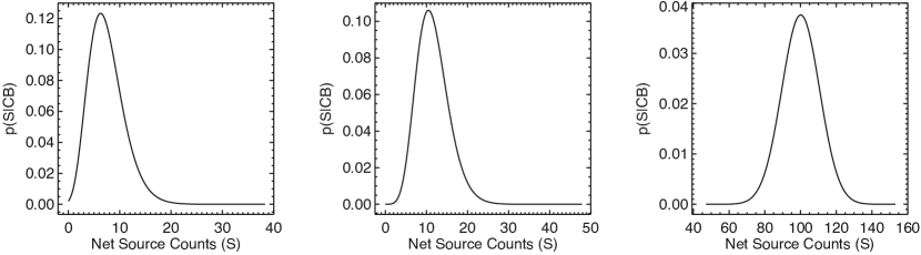
Figure 20.— Probability distributions $p(S|CB)$ for the number of net source counts $S$ in the ACIS broad (b) band for three different CSC source observations. $C$ and $B$ are the total counts in the source and background region apertures, respectively; $\alpha$ and $\beta$ are the fractions of the source counts expected in each aperture; and $r$ is the ratio of the background to source region aperture areas. $p(S|CB)$ is computed as described in the text. Left: $C=7$, $B=41$, $\alpha=0.83731$, $\beta=0.13587$, $r=23.41$ (b band flux significance = 1.94). Center: $C=11$, $B=26$, $\alpha=0.89741$, $\beta=0.08607$, $r=16.36$ (b band flux significance = 3.04). Right: $C=90$, $B=10$, $\alpha=0.89832$, $\beta=0.07743$, $r=24.02$ (b band flux significance = 9.4).

Confidence bounds are determined by numerically integrating $p(S|CB)$ in alternating steps above and below its mode until the desired confidence level is achieved. The values of $S$ at these points then determine the confidence bounds. If the value of $S=0$ is reached before summation is complete, or if the mode itself is 0, integration continues for $S$ above the mode, and the resulting bound is considered an upper limit.

We note that in our approach, photon flux and energy flux are determined somewhat differently. While average exposure map values are used when computing photon flux, in the case of energy flux the values $\langle F_{s}\rangle$ and $\langle F_{b}\rangle$ are determined by applying quantum efficiency and effective area corrections to individual event energies. For sources with few counts in either the source or background region, a single photon detected at an uncharacteristically low or high energy (where the Chandra effective area is small) can make a dominant contribution to the estimated energy flux. In such cases, the true uncertainty will be significantly larger than our estimated errors. A post facto comparison of energy flux estimates computed in this manner with energy fluxes calculated using an assumed canonical power-law spectral model (see § 3.10, below), indicates that fewer than 1% of ACIS broad energy band fluxes are affected by this problem. A more detailed analysis of the statistical accuracy of the energy flux determinations is provided by F. A. Primini et al. (2010, in preparation).

3.7.1 Determining Flux Significance

Significances for all aperture photometry quantities are determined directly from the probability densities $p(S|CB)$. Our goal is to provide a simple statistic that is robust to calculate, easily interpretable by non-expert users, and consistent with the classical SNR definition for high count sources. To this end, we compute the FWHM of $p(S|CB)$, since the latter has a well-defined width even for low-significance sources in the catalog, as shown in Figure 20. If $S=0$ is reached before the half-maximum point below the mode is found, the HWHM is computed from values above the mode and FWHM is set equal to $2\times\mbox{\rm HWHM}$. The FWHM is then used to compute the “equivalent $\sigma$” for a Gaussian probability density,

$$\sigma_{e}=\frac{\mbox{\rm FWHM}}{2\sqrt{2\ln 2}}.$$

The flux significance value that is reported in the catalog for a source is defined to be $\mbox{\rm SNR}=S/\sigma_{e}$, where $S$ is determined from equation (13). This value must be at least 3.0 in at least one energy band for an observation of a source to be included in the first release of the catalog.

The flux significance threshold that we use imposes a conservative limit on sources included in the CSC, which we deem necessary to reduce the number of spurious sources at low count levels to an acceptable value. Comparing our results to those of other large Chandra surveys whose source lists are derived from wavdetect, but whose detection procedures differ, is useful. In Figure 21, we compare the distribution of net counts for CSC sources detected in the ACIS broad ($0.5$–$7.0\rm\,keV$) energy band with distributions of similar quantities for four other Chandra catalogs derived from a range of ACIS exposures comparable to those in the CSC: AEGIS-X (Laird et al., 2009, $0.5$–$7.0\rm\,keV$), the Galactic Center catalog (Muno et al., 2009, $0.5$–$8.0\rm\,keV$), C-COSMOS (Elvis et al., 2009, $0.5$–$7.0\rm\,keV$), and ChaMP (Kim et al., 2007, $0.5$–$8.0\rm\,keV$). We note that while these other catalogs do include sources with fewer net counts than the CSC, the additions are in general not large, comprising $\sim\!5\%$, $\sim\!9\%$, $\sim\!9\%$, and $\sim\!24\%$, for AEGIS-X, the Galactic Center catalog, C-COSMOS, and ChaMP, respectively. We attribute the larger percentage in ChaMP to the restricted fields-of-view and the careful manual screening of source detections used when constructing that catalog. The CSC appears to fare worse in comparison to the XBootes survey (Kenter et al., 2005, $0.5$–$7.0\rm\,keV$), most of whose sources have fewer than 10 net counts. However, the XBootes survey is composed of many $5\rm\,ks$ non-overlapping observations for which the very low ACIS background allows a lower count threshold. In contrast, the CSC is constructed from observations comprising a wide range of exposures, $\sim\!70\%$ of which are greater than $5\rm\,ks$ and $\sim\!10\%$ of which are greater than $50\rm\,ks$. Finally, as mentioned in § 3.4, $\sim\!1/3$ of all sources detected by wavdetect in the ACIS broad energy band fall below the flux significance threshold. However, we expect that a substantial fraction of these sources are spurious.

3.7.2 Combining Aperture Photometry from Multiple Observations

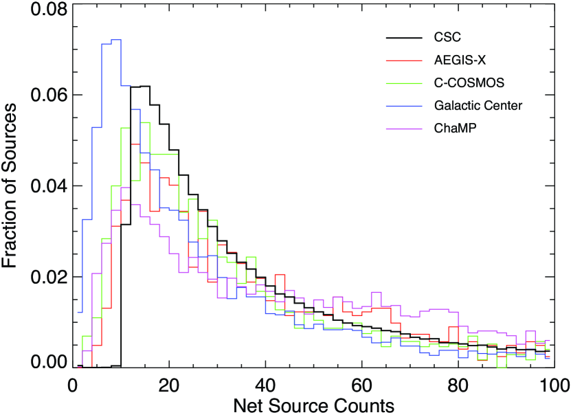
Figure 21.— Comparison of the distribution of net counts for CSC sources detected in the ACIS broad energy band with distributions of similar quantities for four other Chandra catalogs derived from a range of ACIS exposures comparable to those in the CSC.

Ideally, one should compute aperture photometry quantities for combined observations by computing a joint probability density, using $p(S|CB)$ from one observation as the prior for the next. However, this approach is difficult to implement and computationally expensive, especially when probability densities from individual observations do not overlap significantly. We have therefore chosen simply to combine aperture data from various observations and compute a single $p(S|CB)$ from those data. We compute

$$\sum_{i}C_{i}=S\sum_{i}f_{i}+\sum_{i}b_{i} \sum_{i}B_{i}=S\sum_{i}g_{i}+\sum_{i}r_{i}b_{i}.$$ ;

To cast these in the same form as equations (12), we define $r^{\prime}=\sum_{i}r_{i}b_{i}/\sum_{i}b_{i}$, where the $b_{i}$ are determined from the solutions to equations (12) for individual observations. One can then write

$$\sum_{i}C_{i}=S\sum_{i}f_{i}+\sum_{i}b_{i} \sum_{i}B_{i}=S\sum_{i}g_{i}+r^{\prime}\sum_{i}b_{i}.$$ ;

which are identical in form to equations (12). The combined aperture photometry quantities and bounds can then be determined as described earlier.

3.8. Computing Limiting Sensitivity

For the purposes of the catalog, “limiting sensitivity” is defined to be the flux of a point source that meets but does not exceed the flux significance threshold for inclusion in the catalog. Limiting sensitivity is a function of source position, background, and the algorithm used to calculate flux and flux significance. At any point within the field of view of an observation, the limiting sensitivity can be used as a simple X-ray flux limit for individual sources detected at other wavelengths. For the catalog, a full-field sensitivity map is provided for each observation and energy band as a file-based data product (see Table 3). These data are also required to calculate sky coverage histograms (solid angle surveyed as a function of limiting flux), which are themselves needed to calculate luminosity functions and source surface brightness versus number density relationship.

As described above, the flux significance of a catalog source is defined to be the ratio of the source flux to the equivalent $\sigma$ determined from the width of the flux’s posterior probability density. There is no equivalent quantity for sensitivity, and for simplicity and ease of computation, we use a technique similar to that developed by Maccacaro et al. (1982) for the Einstein Observatory Medium Sensitivity Survey, namely, we approximate significance using the aperture photometry relations of § 3.7, under the assumption of Gaussian statistics, and use the model background maps, randomized to provide statistics appropriate to the observation in question, to determine aperture counts.

Recall from equation (13) that the flux may be written as

$$S=(rC-B)/(rf-g).$$ (14)

Since $C$ and $B$ are independent random variables, the variance on $S$ may be written

$$\sigma_{S}^{2} = \frac{r^{2}\sigma_{C}^{2}+\sigma_{B}^{2}}{(rf-g)^{2}}=\frac{r^{2}C+B}{(rf-g)^{2}},$$

assuming Gaussian statistics. The significance, $S/\sigma_{S}$ may then be written as

$$S/\sigma_{S}=\frac{(rC-B)}{\sqrt{r^{2}C+B}}.$$ (15)

The limiting sensitivity is found by determining the minimum number of counts $C_{\rm min}$ in the source aperture that yields the flux significance threshold $\mathit{SNR}_{\rm min}$ in equation (15),

$$\mathit{SNR}_{\rm min}=\frac{(rC_{\rm min}-B)}{\sqrt{r^{2}C_{\rm min}+B}},$$

whose solution is

$$rC_{\rm min}=B+\frac{r\mathit{SNR}_{\rm min}^{2}}{2}\left\{1+\sqrt{1+\frac{4B}{r\mathit{SNR}_{\rm min}^{2}}\left(1+\frac{1}{r}\right)}\right\},$$

and the limiting sensitivity for that aperture is then given by equation (14),

$$\!\!\!\!\!\!\!\!\!\!\!S_{min} = (rC_{min}-B)/(rf-g)$$ (16)

$$= \frac{r\mathit{SNR}_{min}^{2}}{2}\left\{1+\sqrt{1+\frac{4B}{r\mathit{SNR}_{min}^{2}}\left(1+\frac{1}{r}\right)}\right\}$$

$${}\times(rf-g)^{-1}$$

$$= \frac{\mathit{SNR}_{min}^{2}}{2f}\left\{1+\sqrt{1+\frac{4B}{r\mathit{SNR}_{min}^{2}}\left(1+\frac{1}{r}\right)}\right\},$$

where we have approximated

$$(rf-g)^{-1}\approx(rf)^{-1}\left\{1+\frac{g}{rf}\right\}\approx(rf)^{-1}.$$

Since the limiting sensitivity maps are computed from background maps with no real sources, information about real source apertures is unavailable. Rather, for each element in the map, circular source and annular background apertures appropriate to the 90% ECF source aperture at that location are constructed, and used to determine $B$, $r$, and $f$ for use in equation (16).

The assumption of Gaussian statistics, and the subsequent simplification in the algorithm, is made of necessity, since limiting sensitivity must be computed not for each source but for each pixel in each of 5 energy band images. We have, however, verified the performance of the algorithm by comparing detected source fluxes with values of limiting sensitivity at the source locations, for thousands of catalog sources in all energy bands (F. A. Primini et al. 2010, in preparation), and find good agreement.

3.9. Spectral Model Fits

For observations of sources with at least 150 net counts in the energy band $0.5$–$7\rm\,keV$ obtained using the ACIS detector, we further characterize the intrinsic source properties by attempting to fit the observed counts spectrum with both an absorbed black-body spectral model and an absorbed power-law spectral model. These two models represent basic spectral shapes of thermal and non-thermal X-ray emission.

The standard forward fitting method used in X-ray spectral analysis computes the predicted counts produced by the spectral model with the observed counts in the detector channel space, and iteratively refines the model parameters to improve the quality of the fit.

Instrumental response functions (Davis, 2001a) define the mappings between physical (source) space and detector space. George et al. (2007) describe two of these calibration files, the detector redistribution matrix file (RMF) and the ancillary response file (ARF). The former specifies the energy dispersion relation $R(E^{\prime},\hat{p}^{\prime};E,\hat{p},t)$ that defines the probability that a photon of actual energy $E$, location $\hat{p}$, and arrival time $t$ will be observed with an apparent energy $E^{\prime}$ and location $\hat{p}^{\prime}$, while the instrumental effective area $A(\hat{p}^{\prime};E,\hat{p},t)$ is recorded in the latter. The final dispersion relation is the photon spatial dispersion $P(\hat{p}^{\prime};E,\hat{p},t)$ transfer function due to the instrumental point spread function.

With these definitions, the model $M(E^{\prime},\hat{p}^{\prime},t)$ that describes the expected distribution of counts arriving at the detector is then

$$\!\!M(E^{\prime},\hat{p}^{\prime},t)=$$

$$\int dE\,d\hat{p}\,R(E^{\prime};E,\hat{p},t)\,P(\hat{p}^{\prime};E,\hat{p},t)\,A(E,\hat{p}^{\prime},t)\,S(E,\hat{p},t),$$

where $S(E,\hat{p},t)$ is the physical model that defines the physical energy spectrum, spatial morphology, and temporal variability of the source.

We follow standard practice by ignoring the dependency on photon arrival time, and instead consider only the total number of photons that arrived during the observation in the forward fitting process. The source position and shape are taken as known, and we assume that the source photons are collected from the detector area containing an entire source region of interest. The latter assumption is valid provided that sources are spatially separated on scales of order the size of the PSF or larger. In crowded fields, or for sources that have a complex diffuse structure, the contribution from the other sources are important. With the assumptions listed above, equation (3.9) reduces to

$$M(E^{\prime})=\int dE\,R(E^{\prime};E)\,A(E)\,S(E),$$

where the source emitted spectrum $S(E)$ depends on the source physics. The forward fitting procedure solves for the best fit parameters for $S(E)$, assuming a pre-defined fit statistic. Since spectral fitting is only performed for sources with a minimum of 150 net counts, a $\chi^{2}$ fit statistic is used, but note that this assumes a Gaussian distribution for the source counts.

For all sources observed using the ACIS detector (i.e., not just those with at least 150 net counts in the broad energy band), the catalog processing pipelines extract the observed energy spectra of the photons included in the source and background regions of each detected source and store these in a standard format (PHA file; Arnaud & George, 2009). An appropriate associated ARF and RMF are computed by weighting the instrumental responses based on the history of how the source and background regions move over the surface of the detector due to the spacecraft dither motion. The extracted spectra, and associated ARF and RMF are stored as file-based data products (see Table 3) and can be retrieved by the user for further analysis such as low-count spectral fitting or spectral stacking.

To fit the background subtracted data, each PHA spectrum is grouped to a minimum of 16 counts per channel bin, and the source model parameters are varied to minimize the $\chi^{2}$ statistic (assuming data variance, $\sigma_{i}^{2}=N_{i,S}+(A_{S}/A_{B})^{2}N_{i,B}$). Two models are applied to the data in order to evaluate source properties: (1) an absorbed blackbody model $f(E)=\exp^{-N_{\rm H}\sigma_{E}}\,A(E^{2}/(\exp^{E/kT}-1))$; and (2) an absorbed power law model $f(E)=\exp^{-N_{\rm H}\sigma_{E}}\,A\,E^{-\Gamma}$. In these models, $N_{\rm H}$ is the equivalent Hydrogen column density, $\sigma_{E}$ is the photo-electric cross-section based on Balucinska-Church & McCammon (1992) and metal abundances from Anders & Grevesse (1989), $A$ is the model normalization at $E=1\,\rm keV$, $kT$ is the blackbody temperature, and $\Gamma$ is the power-law photon index. Forward fitting is performed using the Sherpa fitting engine (Freeman et al., 2001; Doe et al., 2007). Sherpa finds the best fit model parameters and calculates two-sided confidence intervals for each significant parameter. The model flux for the best fit parameters over the energy range $0.5$–$7\,\rm keV$ is also calculated.

The $68\%\,(1\,\sigma)$  confidence limits for each parameter are calculated using the “projection” method in Sherpa. This method finds the two-sided confidence bounds independently for each parameter. The algorithm assumes that the current model has been fitted, and that all of the parameters are at the values corresponding to a best fit which is at the minimum of the fit statistic ($\chi^{2}_{\rm min}$). For each parameter of interest, the search for the lower or upper bound starts at the best fit value, which is then varied along the parameter axis. At each new value, the parameter of interest is frozen and a new best fit model is determined by minimizing $\chi^{2}$ over the remaining thawed parameters. The new $\chi^{2}$ statistic, $\chi^{2}_{\rm new}$, is determined and the difference between the new and the minimum statistics, $\Delta\chi^{2}=\chi^{2}_{\rm new}-\chi^{2}_{\rm min}$, is calculated. A change in $\Delta\chi^{2}$ equal to 1 corresponds to a $68\%$ confidence bound (Avni, 1976), so the parameter of interest is varied until this value of $\Delta\chi^{2}$ is obtained.

We note here that energy-dependent aperture corrections are not applied when performing the spectral model fits. Since the Chandra PSF is somewhat more extended at higher energies, the lack of correction has the effect of slightly softening the calculated spectral slope. The correction in $\Gamma$ is approximately 0.03–0.05 for power-law spectra with a wide range of spectral indices. For sources included in release 1 of the CSC for which spectral fits have been performed, the error in $\Gamma$ introduced by not applying energy-dependent aperture corrections is roughly six times smaller than the median computed $1\,\sigma$ confidence limits. About 2.5% of sources with spectral fits have computed confidence limits $\lesssim 0.05$, and these cases appropriate caution should be exercised when using the spectral fit properties.

For most source properties, values recorded in the Master Sources Table are computed by combining the relevant data from the set of observations in which the source is detected. However, for simplicity, the spectral model fit parameter values recorded in the Master Sources Table are taken directly from the single observation of the source that has the highest significance, equation (15). In this case, data from multiple observations are not combined to compute the Master Source Table spectral fit properties.

3.10. Spectral Model Energy Fluxes

Spectral model fits are not performed for sources with $<150$ net counts. However, for all sources we estimate energy fluxes using canonical absorbed power-law and black-body spectral models.

For a canonical source model $S(E)$ whose integral over the energy band is $S^{\prime}$, an corresponding band count rate, $C^{\prime}$ in $\rm counts\,s^{-1}$, can be computed from the effective area calibration, $A(E)$, and the RMF, $R(E^{\prime},E)$. The count rate is $\int dE\,R(E^{\prime};E)\,A(E)\,S(E)$, where the integral is performed over the energy band. For HRC observations, a diagonal RMF is assumed. The actual flux of a source can be estimated from $S^{\prime}$ by scaling the latter by the ratio of the measured and modeled source aperture count rates in the energy band. Since the only free parameter in this case is the normalization of the model, the calculation can be performed for sources with too few counts for a reliable spectral fit.

The canonical power-law spectral model has a fixed photon index $\Gamma=1.7$, which falls in the range of values ($\Gamma\sim\!1.5$–2.5) that are typical of AGN spectra (Ishibashi & Courvoisier, 2010). The value chosen matches the photon index used to convert count rates to energy fluxes in the second XMM-Newton serendipitous source catalog (2XMM; Watson et al., 2008), to simplify comparison of CSC and 2XMM source fluxes. Since we anticipate that the majority of sources with spectra that are best fit by a power-law model are AGN, we fix the total neutral Hydrogen absorbing column $N_{\rm H}$ equal to the Galactic column, $N_{\rm H}({\rm Gal})$, under the assumption that this represents a lower limit to the true column density.

The canonical black-body spectral model has a fixed temperature $kT=1.0\rm\,keV$ and total neutral Hydrogen column density $N_{\rm H}=3\times 10^{20}\rm\,cm^{-2}$. The latter value matches the median column density identified by Saxton (2003), and also corresponds to the typical column density found within $1\rm\,kpc$ of the Sun (Liszt, 1983). As discussed by McCollough (2010), the choice of black-body temperature is a compromise between the possible ranges of values for different classes of thermal X-ray emitters. Sources for which a thermal model best represents the data will likely lie in our galaxy, and so in this case setting $N_{\rm H}=N_{\rm H}({\rm Gal})$ would overestimate the total neutral Hydrogen absorbing column.

Similar to spectral model fits, master source spectral model energy fluxes are taken directly from the single observation of the source that has the highest significance.

3.11. Spectral Hardness Ratios

While the spectral model fits described in § 3.9 provide detailed information about a source’s spectral properties, only about 10% of the source observations included in the CSC have sufficient net counts to perform the fitting process. As an aid to characterizing the spectral properties of the remaining catalog sources, hardness ratios are computed between the hard, medium, and soft energy bands for all sources observed with the ACIS detector.

The spectral hardness ratio for the pair of energy bands $x$ and $y$ is defined as

$$\mathcal{HR}_{xy}=\frac{F_{x}-F_{y}}{F_{b}},$$ (18)

where $F_{x}$ and $F_{y}$ are the photon fluxes measured in the energy bands $x$ and $y$ respectively ($x$ is always the higher-energy band of the pair), and $F_{b}$ is the photon flux in the ACIS broad energy band, $F_{b}=F_{h}+F_{m}+F_{s}$.

A catalog source may be readily detected in one or more energy bands, but remain undetected or include very few total counts in other bands. Since hardness ratios are cross-band measures, a technique that applies rigorous statistical methods in the Poisson regime is required to compute these values and their associated confidence limits robustly. The hardness ratios included in the CSC are computed using a Bayesian approach developed by Park et al. (2006), which should be consulted for a detailed description of the algorithm.

To ensure that the Poisson errors are propagated correctly, the conversion between counts and photon flux for each energy band is modeled as a linear process, with a scale factor that is determined from the effective area of the telescope/instrument combination computed at the monochromatic effective energy of the band. This implies that the photon fluxes in equation (18) may not match exactly the aperture photometry fluxes derived in § 3.7.

Specifically, we model the observed total and background counts, $C_{x}$ and $B_{x}$, in the hard, medium, and soft ACIS energy bands as

$$C_{x} \!\sim\! {\rm Poisson}[e_{x}(\lambda_{x}+\xi_{x})],$$

$$B_{x} \!\sim\! {\rm Poisson}[re_{x}\xi_{x}],$$

where $x$ represents the energy band (one of h, m, or s); $\lambda_{x}$ and $\xi_{x}$ are the expected source and background counts intensities, respectively; $e_{x}$ are the conversion factors that scale counts to photon fluxes; and $r$ is the ratio of the background aperture area to the source aperture area.

With these definitions, the spectral hardness ratio for the pair of energy bands $x$ and $y$ is determined by computing the expectation value

$$\mathcal{HR}_{xy}=\frac{\lambda_{x}-\lambda_{y}}{\lambda_{h}+\lambda_{m}+\lambda_{s}}.$$

Table 6Intra-Observation Variability Indices

Variability	Condition	Meaning
Index
0	$p_{\rm GL}\leq 0.5$	Definitely not variable
1	$0.5<p_{\rm GL}<0.667$ AND $f_{3}>0.997$ AND $f_{5}=1.0$	Not considered variable
2	$0.667\leq p_{\rm GL}<0.9$ AND $f_{3}>0.997$ AND $f_{5}=1.0$	Probably not variable
3	$0.5\leq p_{\rm GL}<0.6$ AND ($f_{3}\leq 0.997$ OR $f_{5}<1.0$)	May be variable
4	$0.6\leq p_{\rm GL}<0.667$ AND ($f_{3}\leq 0.997$ OR $f_{5}<1.0$)	Likely to be variable
5	$0.667\leq p_{\rm GL}<0.9$ AND ($f_{3}\leq 0.997$ OR $f_{5}<1.0$)	Considered variable
6	$0.9\leq p_{\rm GL}$ AND $O<2.0$	Definitely variable
7	$2.0\leq O<4.0$	Definitely variable
8	$4.0\leq O<10.0$	Definitely variable
9	$10.0\leq O<30.0$	Definitely variable
10	$30.0\leq O$	Definitely variable

Following the lead of Park et al. (2006), the joint posterior probability distribution can be written as

$$p(\lambda_{s},\lambda_{m},\lambda_{h} \!\!|C_{s},C_{m},C_{h},B_{s},B_{m},B_{h})=$$

$$p(\lambda_{s}|C_{s},B_{s})p(\lambda_{m}|C_{m},B_{m})p(\lambda_{h}|C_{h},B_{h}),$$

where we have made use of the fact that the $\lambda_{x}$ are independent. Marginalizing over nuisance variables yields the posterior distribution for the hardness ratios (equivalent to equation [14] of Park et al., 2006):

$$p(\mathcal{HR}_{xy} \!\!|C_{s},C_{m},C_{h},B_{s},B_{m},B_{h})\,d\mathcal{HR}_{xy}=$$

$$d\mathcal{HR}_{xy}\,\int_{\psi,\omega}\left[d\psi\,d\omega\,\left(\frac{2}{\omega}\right)\right.$$

$$\left.{}\times p(\mathcal{HR}_{xy},\psi,\omega|C_{s},C_{m},C_{h},B_{s},B_{m},B_{h})\vphantom{\left(\frac{2}{\omega}\right)}\right],$$

where $\psi=\lambda_{x}+\lambda_{y}$ and $\omega=\lambda_{s}+\lambda_{m}+\lambda_{h}$.

The spectral hardness ratios that are included in the CSC are determined separately for each observation in which a source is detected, and also from the ensemble of all observations of the source. The former quantities are recorded in the Source Observations Table, while the latter are recorded in the Master Sources Table. The prior probability distributions used to derive the Bayesian posterior probabilities are computed differently in these two cases.

For a single observation, non-informative conjugate $\gamma$-prior distributions (van Dyk et al., 2001) are used for the source and background intensities. These distributions ensure that the posterior probabilities conjugate to the expected Poisson distributions of counts with no other prior information. When multiple observations are combined, the ensemble hardness ratios are computed by stepping through all of the observations of a source in order of increasing net broad-band source counts. The posterior probability distribution computed from each observation is used as the prior probability distribution for the subsequent step. If the propagated prior probability distribution is not consistent with the observed counts in any step, then a conjugate $\gamma$-prior is used instead, and a catalog flag is set to indicate that the source spectrum is variable.

3.12. Estimating Source Variability

The CSC includes estimates of the probability that the flux from a source is temporally variable both within a single observation and between two or more observations in which the source was detected. These estimates are distinguished not only by the fact that they measure variability on different time scales, but also because their definitions differ fundamentally. Within an observation, we measure the probability that the source flux is not consistent with a constant level during a (largely) continuous observation, which is equivalent to estimating the probability that the source is variable, and is a positive statement with respect to variability. The inter-observation variability estimates measure the probability that the average flux levels during the different observations are consistent with a uniform source intensity. This provides only a lower limit to the probability of the source being variable, since we have no information about the source’s behavior during the gaps between the observations, which are often widely separated.

The intent of the various variability measures included in the CSC is to provide users a means to easily select potentially variable sources. The individual source light curves or event lists should be assessed to reveal the true nature of the source’s temporal characteristics. Moderately intense background flares that are not rejected as part of the enhanced background event screening (see § 3.2) may cause sources to be incorrectly identified as variable. This possibility can be evaluated by comparing the structure of the source and background light curves.

3.12.1 Intra-Observation Variability

The probability that a source is variable is estimated separately in each energy band using the Gregory-Loredo and Kolmogorov-Smirnov (K-S) algorithms, and Kuiper’s variation on the latter. A brief description of each of the three algorithms is provided below. Gregory-Loredo probabilities are used to construct intra-observation variability indices that provide a shorthand measure of variability.

All three algorithms directly use the photon event arrival times to compute the variability probabilities, and apply corrections for variations of the geometric areas of the source and background region apertures due to the spacecraft dither-induced motion during the observation. The latter corrections are necessary since a source region that is moving across the edge of the detector or over a bad detector region might otherwise be erroneously classified as variable. Optimal resolution light curves are generated as by-products of the Gregory-Loredo test, and their power spectra are evaluated for the presence of the fundamental spacecraft pitch and yaw dither frequencies or associated beat frequencies. If there is a peak in the power spectrum at one of these frequencies that is at least $5\times$ the RMS value, then a catalog warning flag is set for the source observation to indicate that the intra-observation variability properties are unreliable.

The K-S test (Massey, 1951) is a familiar and well established robust test for comparing two distributions that are a function of a single variable. In the simplest case we compare the cumulative sum of photon events, as a function of time, against a linearly increasing function that represents a constant flux. This null-hypothesis function is modified as necessary to account for data gaps and variations in effective area.

For an observation with $N$ events, let $S_{N}(t)$ be the cumulative sum of detected events as a function of time $t$, and $P(t)$ the cumulative function that represents a constant flux. The K-S statistic $D_{N}$ is defined as

$$D_{N}=\sup_{t}{|S_{N}(t)-P(t)|}.$$

The K-S derived probability that the two distributions $S_{N}(t)$ and $P(t)$ do not belong to the same population, and therefore that the source is variable, is given by

$$p_{\rm var}=Q_{\rm KS}(\sqrt{N}D_{N})$$ (19)

where

$$Q_{\rm KS}(\lambda)=2\sum_{j=1}^{\infty}{(-1)^{j-1}\,e^{-2j^{2}\lambda^{2}}}.$$

Equation (19) is strictly valid only in the asymptotic limit as $N\rightarrow\infty$. In practice $N\gtrsim 20$ is “large enough,” especially if conservative significance levels $\lesssim 0.01$ are required (e.g., Press et al., 1986).

Kuiper (1962) proposed a variation on the K-S test that involves replacing the expression for $D_{N}$ by the difference between the largest positive and negative deviations,

$$D_{N}=\sup_{t}[S_{N}(t)-P(t)]-\inf_{t}[S_{N}(t)-P(t)].$$

Folding this expression into equation (19) yields the Kuiper derived probability that the source is variable. While the K-S test is primarily sensitive to differences between the median values of the cumulative distribution functions, the Kuiper test statistic is as sensitive to differences in the tails of the distributions. In many cases, this makes the Kuiper test a more robust variation of the traditional K-S test for evaluating the probability that a source is variable.

The Gregory-Loredo test (Gregory & Loredo, 1992) is based on a Bayesian approach to detecting variability. The method works very well on photon event data and is capable of dealing with data gaps. We have incorporated the capability to include temporal variations in effective area. Although the algorithm was developed for detecting periodic signals, it is a perfectly suitable method for detecting random variability by forcing the period to equal the length of the observation.

Briefly, the Gregory-Loredo algorithm bins the $N$ observed photon events into a series of histograms containing $m$ bins, where $m$ runs from 2 to $m_{\rm max}$. If the observed distribution of events across the $m$ histogram bins is $n_{1},n_{2},\ldots,n_{m}$, then the probability that this distribution came about by chance can be determined from the ratio of the multiplicity of the distribution, $N!/(n_{1}!\cdot n_{2}!\cdots n_{m}!)$, to the total number, $m^{N}$, of possible distributions. The inverse of this ratio is a measure of the significance of the distribution. Following Gregory & Loredo (1992), we calculate an odds ratio $O_{m}$ for $m$ bins versus a flat light curve as

$$O_{m}=T\;\frac{N!\;(m-1)!}{(N+m-1)!}\ \frac{S_{m}\;m^{N}}{W_{m}},$$ (20)

where we have rewritten the multiplicity of the distribution, $W_{m}$, as

$$W_{m}=\frac{N!}{\prod_{j=1}^{m}{n_{j}!}}.$$

Data gaps are accounted for through the binning factor, $S_{m}$, which is (Appendix B of Gregory & Loredo, 1992)

$$S_{m}=\prod_{j=1}^{m}{s_{j}}^{-n_{j}},$$

where

$$s_{j}=\frac{t_{j}}{T/m},$$

$t_{j}$ is the amount of good exposure time in bin $j$, and $T$ is the total good exposure time for the observation. The odds are summed over all values of $m\geq 2$ to determine the odds that the source is time-variable. $m_{\rm max}$ is chosen for each case in such a way that the odds ratios corresponding to higher values of $m$ contribute negligibly to the total. The probability, $p_{m}$, of a particular binning, $m$, is simply

$$p_{m}=O_{m}/\sum_{j=1}^{m_{\rm max}}O_{j}.$$

Summing over bins $m\geq 2$ corresponding to a non-constant source flux yields the Gregory-Loredo variability probability

$$p_{\rm GL} = \sum_{j=2}^{m_{\rm max}}p_{j}$$ (21)

$$= \frac{O}{1+O},$$ (22)

where $O=\sum_{j=2}^{m_{\rm max}}O_{j}$, and we have made use of the fact that $O_{1}=1$.

Table 7Inter-Observation Variability Indices

Variability	Reduced $\chi^{2}$
Index	2 Observations		$>2$ Observations
0		$<0.4$		$<0.8$
3	$\geq 0.4$	$<0.7$	$\geq 0.8$	$<1.0$
4	$\geq 0.7$	$<1.0$	$\geq 1.0$	$<1.15$
5	$\geq 1.0$	$<2.7$	$\geq 1.15$	$<2.1$
6	$\geq 2.7$	$<7.0$	$\geq 2.1$	$<3.8$
7	$\geq 7.0$	$<12.0$	$\geq 3.8$	$<5.5$
8	$\geq 12.0$		$\geq 5.5$

The Gregory-Loredo algorithm bins the events into a series of light curves of varying resolution, corresponding to the number of bins, $m$, in the range 2 to $m_{\rm max}$. Using the definitions above, the bins that comprise the normalized light curve, $h_{m}$, associated with a specific value of $m$ are

$$h_{j,m}=\frac{n_{j}}{s_{j}N},$$

and the corresponding standard deviations derived from the posterior distribution are

$$\sigma_{j,m}=\frac{1}{s_{j}}\sqrt{\frac{s_{j}h_{j,m}(1-s_{j}h_{j,m})}{N+m+1}}.$$

As described by Gregory & Loredo (1992), an optimal resolution, light curve, $h$, can be obtained by combining the individual light curves, $h_{m}$, weighted by the probabilities, $p_{m}$:

$$h=(1-p_{\rm GL})h_{1}+\sum_{j=2}^{m_{\rm max}}p_{m}h_{m}.$$

The optimal resolution light curve computed from the events included in the source region aperture for each source is recorded as a file-based data product (see Table 3) that is accessible through the catalog. As well as the light curve, $h$, this data product includes the uncertainty, $\sigma$, and upper and lower confidence intervals, $h-3\,\sigma$, and $h+3\,\sigma$, respectively. To allow the users to verify the significance of features that may be present in the light curve, the file also includes the corresponding quantities derived from the events extracted from the background region aperture, using the same binning.

Careful judgement should be applied when assessing the reliability of source variability indicators using the source and background light curves. Since the background region aperture may contain up to $\sim\!10\%$ of the source flux (see § 3.4.1), the background and source light curves may appear similar for very bright sources. The PSF wings of unrelated but nearby strongly variable sources may contaminate both the source and background region apertures of the source being investigated. An observation may have experienced background variations intense enough to be noticeable when compared to the target source’s count rate, but not strong enough to have been removed by background screening during observation recalibration. In the first case the source is truly variable, but this is not necessarily so in the latter two examples. A helpful, though not definitive, test is to scale the amplitude of the flux variations in the source and background region apertures by their respective areas (recorded in the FITS keyword APERTURE). If the variations of the two scaled amplitudes are similar, then there is a good chance that a background problem is responsible. If the source region scaled amplitude is considerably larger than the background region scaled amplitude and the source is strong, then one is likely to have a truly variable source.

The Gregory-Loredo test appears to provide a more uniform and reliable measure of variability than either the K-S or Kuiper tests, although the Gregory-Loredo algorithm is more “conservative” than the other tests. In cases where the K-S and/or Kuiper tests detect variability, but the Gregory-Loredo test does not, close inspection of the light curve often, but not always, demonstrated that the level of variability does not exceed the $3\,\sigma$ bounds on the light curve. In cases where there are considerable data gaps, Gregory-Loredo is not always be able to detect variability on time scales comparable to those gaps.

To provide the user with a short-hand measure of variability that allows selection of sources on different degrees of confidence, the CSC includes a set of integer “variability index” values in the range $[0,10]$. These indices are based on a combination of the Gregory-Loredo probability, $p_{\rm GL}$, the logarithm of the odds ratio, $O$, and a secondary criterion that addresses the overall deviation of the light curve from the mean value. The latter criterion is based on the parameters $f_{3}$ and $f_{5}$, which are the fractions of the light curve that falls within $3\,\sigma$ and $5\,\sigma$ of the average rate, respectively. Table 6 defines the mapping of the test parameters to variability index values.

3.12.2 Inter-Observation Variability

Inter-observation variability is based on comparison of source region aperture photon fluxes, and their confidence intervals, from multiple observations in which the source is detected. The catalog provides a probability that the data are not consistent with a constant-flux source, as well as an inter-observation variability index that is similar to the index defined for intra-observation variability. These measures of variability are assessed for each spectral energy band independently, and consequently no cross-instrument comparison is performed. In the first release of the CSC, observations that cover the same region of the sky, but in which the source is not detected, are not considered when computing inter-observation variability. These observations should enter into the variability assessment as flux upper limits, since they could conceivably be inconsistent with a constant source flux. A future release of the catalog will address this limitation.

As mentioned above, the inter-observation variability probability must be interpreted differently from the intra-observation variability probability. Whereas the light curve can be used to declare a source to be variable or non-variable within the time range of a single observation, one can never conclude that a source does not vary between multiple observations. If inter-observation variability is detected, then the source is definitely variable; however the converse is not true.

Table 8Source Codes

Property	Bit Encoding
conf_code	0: Source is not confused
	1: Multiple source in source region
	2: Source region overlaps another source region
	4: Source region overlaps another background region
	8: Background region overlaps another source region
	16: Background region overlaps another background region
edge_code	0: Source does not dither off detector boundary
	1: Source position dithers off detector boundary
	2: Source region dithers off detector boundary
	4: Background dithers off detector boundary
multi_chip_code	0: Source does not dither between detector chips
	1: Source position dithers across 2 chips
	2: Source region dithers across 2 chips
	4: Background region dithers across 2 chips
	8: Source position dithers across $>2$ chips
	16: Source region dithers across $>2$ chips
	32: Background region dithers across $>2$ chips
var_code	0: Intra-observation source variability not detected in any band
	1: Intra-observation variability detected in the ACIS ultrasoft (u) energy band
	2: Intra-observation variability detected in the ACIS soft (s) energy band
	4: Intra-observation variability detected in the ACIS medium (m) energy band
	8: Intra-observation variability detected in the ACIS hard (h) energy band
	16: Intra-observation variability detected in the ACIS broad (b) energy band
	32: Intra-observation variability detected in the HRC wide (w) energy band

The inter-observation variability probability is simply based on the reduced $\chi^{2}$ of the distribution of the source region aperture photon fluxes of the individual observations and their confidence intervals. For a source detected in $n$ separate observations, we first use the source region aperture photon flux, $S_{i}$, and the associated lower and upper $1\,\sigma$ confidence limits, $S_{i}^{-}$ and $S_{i}^{+}$, respectively, to compute an initial estimate of the variance-weighted mean source region aperture photon flux

$$S_{0}=\sum_{i=1}^{n}\frac{S_{i}}{\sigma_{0,i}^{2}}/\sum_{i=1}^{n}\frac{1}{\sigma_{0,i}^{2}},$$

where we take $\sigma_{0,i}=(S_{i}^{+}-S_{i}^{-})/2$. Using this estimate of the mean flux, we define the “effective $\sigma$” for the $i$th observation of the source as

$$\sigma_{i}=\left\{\begin{array}[]{c l}S_{i}-S_{i}^{-}&\quad S_{i}>S_{0}\\ S_{i}^{+}-S_{i}&\quad S_{i}<S_{0}\\ (S_{i}^{+}-S_{i}^{-})/2&\quad S_{i}=S_{0}.\end{array}\right.$$

A refined estimate of the variance-weighted mean flux is then given by

$$S=\sum_{i=1}^{n}\frac{S_{i}}{\sigma_{i}^{2}}/\sum_{i=1}^{n}\frac{1}{\sigma_{i}^{2}}.$$

and the reduced $\chi^{2}$ is

$$\chi^{2}=\frac{1}{n-1}\sum_{i=1}^{n}\frac{(S_{i}-S)^{2}}{\sigma_{i}^{2}}.$$

The inter-observation variability index is assigned on the basis of the reduced $\chi^{2}$, according to Table 7. Note that the values 1, 2, 9, and 10 are not used.

3.13. Source Codes and Flags

Each entry in both the Master Sources Table and the Source Observations Table includes several source-specific flags and codes that identify specific circumstances that may be of relevance to the catalog user. Some flags and codes are used to encode source properties that are commonly searched for by users, as an aid to simplify catalog queries. However, in most cases flags and codes are intended to warn the user of conditions that may degrade the quality of measured source properties, or that may limit the usefulness of the source detection for some investigations.

The codes and flags included in the Source Observations Table are defined in Table 1. Flags are Boolean quantities that describe “yes/no” or “true/false” properties, whereas codes are multi-bit data values that encode several levels of information. Translations of the bit-encodings can be found in Table 8.

The extent and variability codes require additional explanation. The former encodes a conservative estimate of whether the intrinsic extent of a source, $a_{\rm rss}$ [equation (10)], is inconsistent with the extent of the local PSF in each energy band. Specifically, a source is considered extended in an energy band if $a_{\rm rss}>5\,\Delta a_{\rm rss}$ in that energy band, where $\Delta a_{\rm rss}$ is the uncertainty in $a_{\rm rss}$, given by equation (3.6.2). The variability code bit corresponding to a specific energy band is set if the intra-observation variability index (Table 6) $\geq 3$. A zero code therefore implies that the source is either definitely not variable, not considered variable, or probably not variable, depending on the value of the variability index. Similarly, a non-zero code implies that the source either may be variable, is likely to be variable, is considered variable, or is definitely variable.

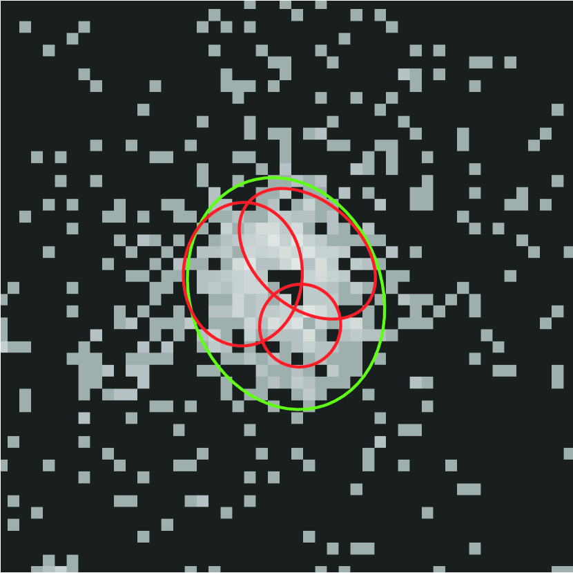
Figure 22.— Example of a highly piled-up source detected using ACIS. The core of the image has been eroded by photon pile-up, so that the source has a cratered appearance (i.e., the photon density has an apparent minimum at the source location). Bright spots on the ring are detected as distinct sources, shown in red. These source detections are manually adjusted to include only a single source centered on the crater, shown in green.

The remaining codes and flags all warn of conditions that may affect derived source properties to some extent. The streak source flag, if set, indicates that the source detection is located on an ACIS readout streak. If the readout streak is associated with a bright source, then there is a significant probability that the source properties may be compromised. This is particularly true of aperture photometry values. If the streak is especially intense, then the source detection may not be real. If the saturated source flag is set, then the source is definitely real, but is so bright that photon pile-up has eroded the core of the source image so that a single source has a “cratered” appearance (Fig. 22). All source properties are compromised.

The Master Sources Table includes only flags, and these are defined in Table 2. In most cases, Master Sources Table flags summarize the corresponding Source Observations Table flags and codes for all of the source detections that have “unique” linkages to the master source. The confusion flag is an exception to this, in that it is set for a master source if the confusion codes for any of the associated source detections indicate that multiple sources are present in the source region or that the source region overlaps another source region, or if there are any source detections that have “ambiguous” linkages to the current master source.

The master extent and variability flags are set if the corresponding codes for any uniquely matched source detections indicate that the source is extended or variable (as appropriate) in any energy band. The remaining master source flags are set only if the corresponding Source Observations Table flags are set for all uniquely associated source detections, indicating that the corresponding warning criteria are violated in all observations of the source.

3.14. Quality Assurance

Table 9ACIS Observation False Source Rate

Configuration	Livetime (ks)	False Source Rate
ACIS-012367	009	0.00
ACIS-235678	010	0.02
ACIS-012367	029	0.00
ACIS-235678	030	0.12
ACIS-235678	051	0.21
ACIS-012367	068	0.22
ACIS-235678	118	1.20
ACIS-012367	125	1.28

The scientific integrity of the CSC is guaranteed through a set of quality assurance steps that are performed as part of the catalog construction process (Evans et al., 2008). Many of these analyses are executed automatically at the completion of each stage of catalog pipeline processing, so that any issues can be identified and corrected before they can affect downstream processing. These mechanisms detect pipeline processing errors, and identify potential data quality issues by comparing key diagnostic output products with predefined standards. Each standard that is violated will either trigger a human review to determine how to proceed, or will initiate one or more automated actions. The latter typically result in termination of the processing thread for a subset of the input data.

The vast majority of violations that occur because of data quality issues address the reality of detected sources, and are typically resolved without human intervention. Following the source detection step, detected source regions that are either significantly smaller than the dimensions of the local PSF or significantly larger than the maximum expected source size, or which exceed a maximum ellipticity threshold, are deemed to be artifacts, and the processing thread for the source region is terminated immediately to avoid evaluating source properties unnecessarily. Sources that have too few counts, or that have a detection significance that is too low to pass the catalog SNR threshold are similarly discarded.

The cores of sources observed with ACIS that are sufficiently bright can be eroded by photon pile-up. The source detection algorithm incorrectly detects bright spots on the ring surrounding the dark center of the image as distinct sources. Saturated sources are identified using a sliding matched filter algorithm. The source detections are manually adjusted so that a single source centered on the crater is included in the Source Observations Table for the source, and the source properties are flagged as having been manually modified, so that the user can exclude such sources if they so wish. The tabulated source position errors are unreliable for sources whose regions have been manually modified.

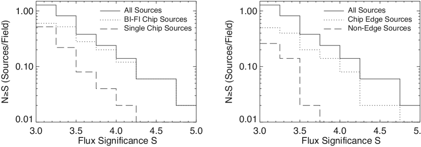
Figure 23.— False source rate as a function of flux significance for a simulated $125\rm\,ks$ observation. The maximum flux significance across all science energy bands is plotted. Left: BI-FI Chip Sources are those whose source regions dither across the CCD S2 (ACIS-6; back-illuminated)–S3 (ACIS-7; front-illuminated) boundary. Single Chip Sources are those whose source regions are completely contained on only a single chip. Right: Chip Edge Sources are those whose source regions dither off a chip edge during the observation. Non-Edge Sources are those whose source and background regions do not dither off a chip edge.

A more detailed comparison of the source dimensions with the local PSF is performed after the source properties are computed, to identify sources that are statistically smaller than the PSF in all energy bands. The fraction of the local PSF that is included within the modified source region aperture (as defined in § 3.4.1) must be sufficiently large that the source location and aperture photometry can be computed from the fraction of the aperture that is not contaminated by overlapping sources. Finally, the SNR of the source is evaluated and compared with the minimum required for inclusion in the catalog.

Human review is primarily required to address the occurrence of unexpected pipeline warnings or errors. Although an automated process performs the laborious task of scanning the log files associated with each processing pipeline to identify problems, the wide diversity of possible error conditions require human intelligence to assess the reason for the failure and determine how to proceed. The typical response is to terminate the current processing thread, perform any needed repairs, and initiate reprocessing of the thread.

Other conditions that trigger a human review are precautionary in nature, and include cases where the local spatial density of detected sources is too high, or the total number of sources detected in the field of view exceeds a predefined threshold. Although these conditions most likely arise because of field crowding, they could indicate an error in the source detection process. Errors that generate a large number of sources would require substantial cleanup if processing was allowed to continue incorrectly.

4. STATISTICAL PROPERTIES

A detailed characterization of the statistical properties of the CSC is beyond the scope of this paper, but is the subject of a comprehensive discussion by F. A. Primini et al. (2010, in preparation). Here, we merely present a summary of the principal statistical properties of the catalog for reference.

Statistical characterization of catalog source properties is accomplished primarily by using simulated and empty field (blank-sky) observations, together with datasets consisting of empty fields that have simulated sources with known properties added. These datasets are processed by the catalog pipelines in the same manner as real observations.

4.1. False Source Rate

To estimate false source rates, a series of blank-sky simulations with exposure times of $\sim\!10$, $30$, $60$, and $120\rm\,ks$ were constructed for typical ACIS imaging CCD configurations. For each simulation, a template background event list for each active CCD was used to define the overall spatial variation of the background, and the total number of background events was determined from the nominal field background rates (Chandra X-ray Center, 2009) and the simulated exposure time. For all CCDs except chip S4 (ACIS-8) the template background event lists recorded in the instrumental calibration database were used. Chip S4 is significantly affected by a variable pattern of linear streaks that appear to be caused by a flaw in the serial readout which randomly deposits significant amounts of charge along pixel rows as they are read out (Houck, 2000). Because of this issue, no adequate template is available for chip S4, and so one was constructed by combining several CSC event lists that do not include bright sources on that CCD. Each simulated blank-sky event list was then processed through the CSC pipeline source detection steps. The false source rates derived from these simulations are reported in Table 9. From these data we derive a simple linear relation for the number of false sources per field as a function of livetime, namely

$$\log(R_{\rm fs})=-3.345+1.6\times\log(t_{\rm live}),$$

where $R_{\rm fs}$ is the false source rate, and $t_{\rm live}$ is the exposure livetime in units of ks. Using this relation, we estimate that $\sim\!370$ sources ($\sim\!0.4\%$) included in the catalog are spurious.

As can be seen from the table, the false source rate is appreciable only for exposures longer than $\sim\!50\rm\,ks$. There is some evidence for a clustering of false source detections near chip edges and at the boundaries between the back- and front-illuminated CCDs. This should not be surprising since the low spatial frequency background is poorly constrained or changing rapidly in these locations. To investigate these effects further, the false source rates near the chip edges and interfaces were examined separately for the longest simulated exposures. Figure 23 demonstrates that false source rates are enhanced in these regions for the $125\rm\,ks$ simulation.

4.2. Source Detection Efficiency

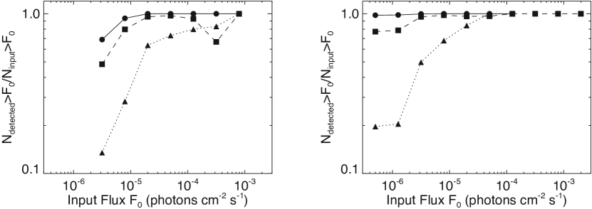
Figure 24.— Cumulative detection efficiency estimates from ACIS-012367 simulations of point sources with absorbed power-law spectral distributions ($\Gamma=1.7$, $N_{\rm H}=3\times 10^{20}\rm\,cm^{-2}$). Simulated source fluxes were drawn from a power-law $N>S$ distribution with index 1.5 and an overall normalization adjusted to yield a few hundred detectable sources per simulation. Thirty simulations per exposure time were calculated. Detection efficiency is computed by comparing the measured and input $N>S$ distributions in the ACIS broad energy band. The ratio of these two distributions represents the fraction of input sources of a given incident flux that are actually detected. Left: Detection efficiency for a $\sim\!9\rm\,ks$ exposure. The solid, dashed, and dotted lines plot the detection efficiencies for sources with $\theta<5^{\prime}$, $5^{\prime}\leq\theta<10^{\prime}$, and $10^{\prime}\leq\theta<15^{\prime}$, respectively. Because of the power-law $N>S$ distribution, relatively few bright sources were simulated and the plotted detection efficiency does not smoothly approach 100% for bright sources because of small number statistics. Right: As for the left panel, except for a $\sim\!125\rm\,ks$ exposure time.

Source detection efficiency is characterized using point source simulations. A spatially random distribution of point sources is added to the blank sky simulations described above using the MARX simulator (Wise et al., 2003) to generate the incident X-ray photons. Separate simulations were generated for non-thermal sources with a power-law spectral distribution $F_{E}\propto\!E^{-1.7}$, and for thermal black-body sources with temperature $kT=1.0\rm\,keV$, spectra. A neutral Hydrogen absorbing column $N_{\rm H}=3\times 10^{20}\rm\,cm^{-2}$ was assumed for all sources. Source fluxes were drawn from a power-law $N>S$ distribution with index 1.5. The overall normalization was adjusted to yield a few hundred detectable sources per simulation, a compromise aimed at reducing source confusion while limiting the total number of simulations required to obtain good statistics. The effects of photon pile-up (Davis, 2001b) and observation-specific bad pixels were included by post-processing each simulation with marxpileup and acis_process_events, respectively. The source events from the MARX simulations were then merged with the appropriate simulated blank-sky event lists, keeping only MARX-simulated source events that fell on active CCDs for the observation. As with the blank-sky simulations, simulated event lists were then processed through the CSC pipeline source detection and source properties extraction steps, and the resulting sources that would have been included in the catalog were tabulated. Finally, these sources were cross-referenced with the input source lists to allow a source-by-source comparison of input and derived properties.

Source detection efficiency is determined by comparing the measured $N>S$ and input $N>S$ distributions. The ratio of these two distributions represents the fraction of input sources of a given incident flux that are actually detected. Results of the comparison for the ACIS broad energy band detections from the shortest and longest ACIS-012367 power-law spectral distribution simulation sets are shown in Figure 24. The standard CSC processing pipeline further combines ACIS source detections from the broad, soft, medium, and hard energy bands to construct the final detected source list. This step was not performed as part of these simulations. However, since the simulated source spectra are homogenous and well detected in the broad energy band, the difference is not significant in this case.

4.3. Absolute Astrometric Accuracy

As mentioned in § 3.5.1, the absolute astrometric accuracy of release 1 of the CSC was evaluated post facto by cross-matching catalog sources with their counterparts from the SDSS DR7 (Abazajian et al., 2009). Like the CSC, the SDSS DR7 is referenced to the International Celestial Reference System (ICRS; Arias et al., 1995), and has statistical positional uncertainties $\sim\!45\rm\,milliarcseconds$ (mas) rms per coordinate for bright stars, with systematic errors $<20\rm\,mas$ (Abazajian et al., 2009). Only CSC-SDSS source pairs with more than 90% match probability, evaluated according to the Bayesian probabilistic formalism described by Budavári & Szalay (2008), were evaluated, resulting in 6,310 source pairs associated with 9,476 sources detected in individual observations. Full details of the analysis and results are presented by Rots (2009) and F. A. Primini et al. (2010, in preparation). Here we summarize the main result.

For each matching CSC-SDSS source pair, the separation, $\rho$, and the total $1\,\sigma$ positon error are computed, summing in quadrature the CSC and SDSS errors (and remembering that CSC position errors are reported as 95% uncertainties). We then examine the value of reduced $\chi^{2}=\sum(\rho/\sigma_{{\rm tot}})^{2}/(n-1)$ for bins in $\sigma_{{\rm tot}}$ covering the range $\sim\!0.1$–$2^{\prime\prime}$. The value of the reduced $\chi^{2}$ is reasonably close to 1, except for $\sigma_{{\rm tot}}\lesssim 0.3^{\prime\prime}$ (indicating that the errors are underestimated in that range). Adding a systematic astrometric error component of $0\farcs 16\pm 0\farcs 0.01$ to $\sigma_{{\rm tot}}$ yields reduced $\chi^{2}$ near 1 for all values of $\sigma_{tot}$. We therefore adopt that value as the systematic astrometric error present in release 1 of the CSC.

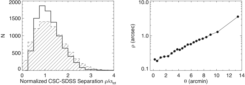
Figure 25.— Left: Distribution of the normalized separations for matching CSC-SDSS source pairs (solid line). The theoretical Rayleigh distribution for the same number of sources is shown hatched. Right: Average CSC-SDSS source pair separation with $0\farcs 16$ systematic astrometric error included, as a function of off-axis angle, $\theta$.

The distribution of the normalized separations for the CSC-SDSS source match pairs is shown in the left panel of Figure 25, together with the theoretical Rayleigh distribution for the same number of sources. The overall shape of the curve agrees with the Rayleigh distribution, although there is a slight deficit at high values of normalized separation, suggesting that the overall error may be overestimated for sources at large off-axis angles. In the right panel of Figure 25, we present the average CSC-SDSS separation as a function of off-axis angle, with the systematic astrometric error included. The average CSC $1\,\sigma$ positional error ranges from $0\farcs 2$ on-axis to $\sim\!3\farcs 5$ at $\sim\!14^{\prime}$ off-axis.

4.4. Photometric Accuracy

To assess the accuracy of CSC source fluxes, the measured source region aperture photon fluxes are compared with the input photon fluxes of the simulated point sources. Figure 26 presents the comparison of ACIS broad energy band photon fluxes for simulated sources with a power-law spectrum. Inspection of the figure reveals good agreement for sources with off-axis angles within $10^{\prime}$ of the aimpoint. For sources beyond $10^{\prime}$, photon fluxes appear to be systematically overestimated by a factor of $\sim\!2$ for sources fainter than $\sim\!3\times 10^{-6}\rm\,photons\,cm^{-2}\,s^{-1}$.

The systematic error in the faint flux bins is more prominent in the ACIS soft energy band, in which the measured fluxes appear under-estimated for all simulated input flux levels. Further investigation of this effect will be reported by F. A. Primini et al. (2010, in preparation). Preliminary analysis suggests that the effect results from the use of a monochromatic exposure map (computed at the effective energy of the band) when determining source fluxes. Models based on this assumption reproduce the general features of the apparent systematic errors, and for the assumed model power-law spectrum the error is $\sim\!10\%$ in the broad, medium, and hard energy bands, $\sim\!20$–$30\%$ in the soft energy band, and $\sim\!30\%$ in the ultra-soft energy band.

5. CONCLUSIONS

The Chandra Source Catalog is a general purpose virtual X-ray astrophysics facility that provides access to a carefully crafted set of scientifically useful quantities for individual X-ray sources observed by the Chandra X-ray Observatory. The first release of the catalog was published to the astronomical community in March 2009, and includes source properties for 94,676 point and compact X-ray sources detected in a subset of public ACIS imaging observations from roughly the first eight years of the Chandra mission. This release of the catalog includes sources with observed spatial extents are $\lesssim 30^{\prime\prime}$, and whose flux estimates are at least 3 times their estimated $1\,\sigma$ uncertainties. Observations that include substantially extended sources are not included in the first release of the catalog. For each X-ray source, the catalog tabulates about 60 distinct measured and derived source properties, generally with associated lower and upper confidence limits, in several energy bands. These properties are generally derived from all of the observations in which a source is detected. However, in the first catalog release, multiple observations are not combined prior to source detection, so the depth of the catalog is limited by the duration of the longest single exposure of a field. The catalog further tabulates roughly 120 observation-specific properties for each observation of a source, again with associated lower and upper confidence limits, and in several energy bands.

Tabulated source properties include source position, spatial extent, multi-band aperture fluxes computed in several different ways, X-ray hardness ratios and spectral model fits, and intra- and inter-observation variability measures. In addition to these “traditional” catalog elements, for each source detection the catalog includes an extensive set of FITS format file-based data products that can be manipulated interactively by the user, including source images, event lists, light curves, and spectra from each observation in which a source is detected.

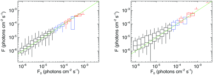
Figure 26.— Comparison of input ($\rm F_{0}$) and measured ($\rm F$) ACIS broad (b) band fluxes for simulated sources with power-law spectra and off-axis angles $\theta\leq 10^{\prime}$ (left) and $\theta>10^{\prime}$ (right). For each bin, the horizontal line indicates the median measured flux value. The boxes include 90% of the measurements in each bin, and the vertical lines indicate the extreme values. Bins colored red include fewer than 100 measurements; bins colored blue include 100–400 measurements; bins colored black include more than 400 measurements. The green line has a slope of 1.

Looking towards the future, release 1.1 of the catalog, scheduled for spring 2010, will include data from public HRC-I imaging observations and newly public ACIS imaging observations, but will otherwise retain the same limitations as release 1. In release 2, we plan to co-add multiple observations of the same field that use the same or similar instrument configurations, and that have similar spacecraft pointings (within $\sim\!30^{\prime\prime}$) prior to source detection, to achieve fainter limiting sensitivities in many fields. We anticipate that new algorithms will allow this release to have a significantly fainter source detection threshold than release 1. This release should also provide limited improvements in the area of extended source handling (for example allowing for the inclusion of exposures containing moderately extended emission from galaxy cores up to $\sim\!60^{\prime\prime}$ spatial scale), as well as numerous algorithm enhancements that will refine field and source property calculations.

Appendix A MASTER SOURCE MATCHING ALGORITHM

The procedure, referenced in § 3.4.2, for matching source detections from multiple observations that overlap the same region of the sky, is described here. These steps must be executed for each observation, but the outcome does not depend on the order in which the observations are processed.

The algorithm defines the overlap ellipse of a source detection to be the PSF 90% ECF aperture in the energy band that has the highest number of aperture source counts. The following two assumptions are made: (a) if a source detection in one observation is resolved into multiple source detections in a second observation, then the overlap ellipse corresponding to the former detection will overlap all of the overlap ellipses corresponding to the latter detections, and (b) multiple source detections in a single observation correspond to distinct sources on the sky, even if the overlap ellipses intersect spatially.

For the set ${\mathcal{S}}$ of source detections identified in the current observation, the following 9 steps are performed.

(1) Identify the sets ${\mathcal{M}}_{i},{\mathcal{M}}_{j},\ldots$ of candidate matching source detections in observations $i,j,\ldots$ that overlap the current observation. Candidate matching source detections are those source detections that have radial separations on the sky from any member of the set ${\mathcal{S}}$ that are smaller than some predefined radius, $r$. For convenience, we designate the union ${\mathcal{M}}_{i}\cup{\mathcal{M}}_{j}\cup\ldots$ as the set ${\mathcal{M}}$.

(2) Compute the overlap ellipses, defined above, for each member of the sets ${\mathcal{S}}$ and ${\mathcal{M}}$.

Two source detections $a$ and $b$ in observations ${\mathit{1}}$ and ${\mathit{2}}$, respectively, are deemed to overlap if and only if

$$A[a\cap b]/A[a]>0.15 {\it or\/} A[a\cap b]/A[b]>0.15,$$

where $A[a]$ is the area of the overlap ellipse of source detection $a$, and $A[a\cap b]$ is the area of the spatial intersection of the overlap ellipses of $a$ and $b$. This has the effect of dismissing very small overlaps.

Figure 27.— Example “confused match” source detections. Source detection $a$ from observation ${\mathit{1}}$, overlaps source detections $b_{1}$ and $c$ from observations ${\mathit{2}}$ and ${\mathit{3}}$, respectively. Source detection $c$ also comprises a partial unambiguous match with source detection $b_{2}$ from observation ${\mathit{2}}$. The latter connection implies that source detections $a$ and $c$ are confused matches with the pair of sources $b_{1}$ and $b_{2}$ from observation ${\mathit{2}}$.

In addition, if a source detection $a$ in observation ${\mathit{1}}$ overlaps multiple source detections $b_{1},b_{2},\ldots,b_{n}$ ($n>{\mathit{1}}$) in observation ${\mathit{2}}$, and

$$A[a\cap b_{i}]/A[a]>0.67 {\it and\/} A[a\cap b_{j}]/A[a\cap b_{i}]<0.33$$

for all $j\neq i$, then only the overlap between source detections $a$ and $b_{i}$ is recognized. The remaining source detections $b_{j}$ included in observation ${\mathit{2}}$ are deemed not to overlap source detection $a$. This has the effect of recognizing only a single dominant overlap and ignoring additional smaller overlaps from the same observation.

(3) Compute the subset ${\mathcal{N}}\subseteq{\mathcal{S}}$ of source detections that do not overlap any member of the set ${\mathcal{M}}$ of candidate matching source detections. ${\mathcal{N}}$ comprises the set of source detections that must be added to the Master Sources Table as newly identified master sources.

(4) Compute the set ${\mathcal{P}}$ of members of ${\mathcal{S}}\cup{\mathcal{M}}$ that comprise partial unambiguous matches. A source detection $a$ included in observation ${\mathit{1}}$ is a partial unambiguous match to a source detection $b$ included in a different observation ${\mathit{2}}$ if and only if (a) $a$ overlaps $b$, (b) $a$ does not overlap any other source detection included in observation ${\mathit{2}}$, and (c) $b$ does not overlap any other source detection included in observation ${\mathit{1}}$. Sources included in ${\mathcal{P}}$ are uniquely matched between pairs of overlapping observations, but are not necessarily uniquely matched between all overlapping observations.

(5) Compute the subset ${\mathcal{U}}\subseteq{\mathcal{P}}$ of unambiguous matches. An unambiguous match between source detections $a,b,c,\ldots$ included in observations ${\mathit{1}},{\mathit{2}},{\mathit{3}},\ldots$ occurs when all pairs $([a,b],[a,c],[a,\ldots],[b,c],[b,\ldots],\ldots)$ of source detections individually form partial unambiguous matches. ${\mathcal{U}}$ comprises the set of source detections that are uniquely matched to existing master sources in the Master Sources Table.

Figure 15, Left is an example of an unambiguous match.

(6) Compute the set ${\mathcal{C}}$ of members of ${\mathcal{S}}\cup{\mathcal{M}}$ that comprise confused matches. A confused match results when a source detection $a$ included in observation ${\mathit{1}}$ overlaps multiple source detections $b,c,\ldots$ that either (a)(i) are included in a single observation ${\mathit{2}}$ and (ii) overlap no other source detection in observation ${\mathit{1}}$ than $a$, or (b) consist of partial unambiguous matches such that there is at least one observation that is common amongst the partial unambiguous matches for all of the sources $b,c,\ldots$. ${\mathcal{C}}$ comprises the set of confused source detections that must be flagged as confused, and linked ambiguously to the corresponding master sources in the Master Sources Table.

An example of case (a) above is shown in Figure 15, Center. In the case (b) above, note that source detection $a$ is not required to overlap all of the individual source detections that comprise each of the partial unambiguous matches (e.g., Fig. 27).

(7) Once the set ${\mathcal{C}}$ of confused matches is determined, steps (2)–(5) should be re-applied to the set $\{{\mathcal{S}}\cup{\mathcal{M}}\}\backslash\{{\mathcal{N}}\cup{\mathcal{U}}\cup{\mathcal{C}}\}$ to identify additional members of the sets ${\mathcal{N}}$ and ${\mathcal{U}}$ that were previously missed because they were overlapped by one or more confused source detections.

(8) After all members of the sets ${\mathcal{N}}$ and ${\mathcal{U}}$ have been identified, re-examine members of the set ${\mathcal{C}}$ to verify that the overlaps of source detections that caused each member to become assigned to set ${\mathcal{C}}$ are overlaps with members of ${\mathcal{N}}$ and ${\mathcal{U}}$. If any source detection which is not a member of ${\mathcal{N}}$ or ${\mathcal{U}}$ overlaps a member of ${\mathcal{C}}$, and that overlap was relied on to assign the member to ${\mathcal{C}}$, then remove the member from set ${\mathcal{C}}$. The removed member will revert to an uncategorized source detection.

(9) At this point, the set $\{{\mathcal{S}}\cup{\mathcal{M}}\}\backslash\{{\mathcal{N}}\cup{\mathcal{U}}\cup{\mathcal{C}}\}$ consists of source detections that cannot be merged or linked to master sources using the above rules. These source detections typically (but not exclusively) overlap at least two other sources that were observed in different observations and that do not overlap each other. We designate members of this set ${\mathcal{H}}$ as human-review matches. Manual review is required to disambiguate the source matches.

Figure 15, Right is an example of a human-review match.

Appendix B COMBINING SOURCE POSITIONS

As described in § 3.5.2, a multivariate optimal weighting formalism is used to improve the estimates of the position and positional uncertainty of each X-ray source by combining the statistically independent source detections included in the set of individual observations. The source position error uncertainties are expressed in the form of error ellipses centered upon the estimated source positions. Details of the derivations can be found in Davis (2007b).

The improved estimates of the source position, $X$, and associated covariance matrix, $\sigma^{2}$, are

$$X=\sigma^{2}\sum_{i}\frac{X_{i}}{\sigma_{i}^{2}} \sigma^{2}=\left[\sum_{i}\frac{1}{\sigma_{i}^{2}}\right]^{-1},$$ ; (B1)

where $X_{i}$ represents the $i$th estimate of the mean of the two-dimensional source position, and $\sigma_{i}^{2}$ denotes the $2\times 2$ covariance matrix, equation (B7) below, associated with this estimate.

Before the covariance matrix $\sigma^{2}$ can be computed, the individual error ellipses must be mapped from the celestial sphere onto a common tangent plane. The $i$th estimate of the source position is specified as a confidence-ellipse centered upon the celestial coordinates $(\alpha_{i},\delta_{i})$, with the major axis of the ellipse making an angle $\theta_{i}$ ($-\pi\leq\theta_{i}<\pi$) with respect to the local line of declination at the center of the ellipse. The celestial coordinates $(\alpha_{i},\delta_{i})$ correspond to a unit vector

$$\hat{p}_{i}=\hat{x}\cos\alpha_{i}\cos\delta_{i}+\hat{y}\sin\alpha_{i}\cos\delta_{i}+\hat{z}\sin\delta_{i}$$

on the celestial sphere, where $(\hat{x},\hat{y},\hat{z})$ are orthonormal basis vectors oriented such that $\hat{x}$ points to the origin of right ascension on the celestial equator, $\hat{z}$ points to the North celestial pole, and $\hat{y}$ completes the right-hand Cartesian system.

The common tangent plane is constructed on the celestial sphere at the position $\hat{p}_{0}$, which is taken to be the arithmetic mean of the ellipse centers $\hat{p}_{i}$:

$$\hat{p}_{0}=\sum_{i}\hat{p_{i}}/\left|\sum_{i}\hat{p_{i}}\right|.$$ (B2)

The tangent plane coordinates ($x_{i}$, $y_{i}$) corresponding to $(\alpha_{i},\delta_{i})$ are

$$x_{i} = (\hat{p}_{i}\cdot\hat{e}_{x})/(\hat{p}_{i}\cdot\hat{p}_{0})$$

$$y_{i} = (\hat{p}_{i}\cdot\hat{e}_{y})/(\hat{p}_{i}\cdot\hat{p}_{0}),$$ (B3)

where $\hat{e}_{x}$ and $\hat{e}_{y}$ are orthonormal basis vectors parallel to the local lines of right ascension and declination at $\hat{p}_{0}$, i.e.,

$$\hat{e}_{x} = -\hat{x}\sin\alpha_{0}+\hat{y}\cos\alpha_{0}$$

$$\hat{e}_{y} = -\hat{x}\sin\delta_{0}\cos\alpha_{0}-\hat{y}\sin\delta_{0}\sin\alpha_{0}+\hat{z}\cos\delta_{0},$$

where $(\alpha_{0},\delta_{0})$ are the celestial coordinates that correspond to $\hat{p}_{0}$.

Similarly, the unit vectors on the celestial sphere corresponding to the end-point positions of the semi-minor and semi-major axes of the ellipse are given by

$$\hat{p}_{i}^{\rm minor} = \hat{p}_{i}\cos\phi_{i}^{\rm minor}+\hat{\alpha}_{i}\sin\phi_{i}^{\rm minor}\cos\theta_{i}-\hat{\delta}_{i}\sin\phi_{i}^{\rm minor}\sin\theta_{i}$$

$$\hat{p}_{i}^{\rm major} = \hat{p}_{i}\cos\phi_{i}^{\rm major}+\hat{\alpha}_{i}\sin\phi_{i}^{\rm major}\sin\theta_{i}+\hat{\delta}_{i}\sin\phi_{i}^{\rm major}\cos\theta_{i},$$ (B4)

where $\phi_{i}^{\rm minor}$ and $\phi_{i}^{\rm major}$ are the arc-lengths of the semi-minor and semi-major axes, respectively, and $\hat{\alpha}_{i}$ and $\hat{\delta}_{i}$ are unit vectors that point along the directions of increasing right ascension and declination, respectively, at the position $\hat{p}_{i}$.

The lengths of the semi-minor and semi-major axes on the tangent plane are given by

$$\sigma^{\prime}_{1,i} = \sqrt{(x_{i}^{\rm minor}-x_{i})^{2}+(y_{i}^{\rm minor}-y_{i})^{2}}$$

$$\sigma^{\prime}_{2,i} = \sqrt{(x_{i}^{\rm major}-x_{i})^{2}+(y_{i}^{\rm major}-y_{i})^{2}},$$ (B5)

respectively, where we have denoted the tangent plane coordinates of $\hat{p}_{i}^{\rm minor}$ and $\hat{p}_{i}^{\rm major}$ as ($x_{i}^{\rm minor}$, $y_{i}^{\rm minor}$) and ($x_{i}^{\rm major}$, $y_{i}^{\rm major}$), respectively. The angle that the semi-major axis makes with respect to the local line of declination is

$$\vartheta^{\prime}_{i}=\tan^{-1}\left(\frac{x_{i}^{\rm major}-x_{i}}{y_{i}^{\rm major}-y_{i}}\right).$$ (B6)

Armed with the projections of the individual error ellipses projected on the common tangent plane, equations (B)–(B6), covariance matrices can be computed as follows.

The three parameters that specify the geometry of each projected error ellipse are the lengths of the semi-major and semi-minor axes, and the position angle $\vartheta$ that the major axis of the ellipse makes with respect to the tangent plane $y$ axis. The semi-major and semi-minor axis lengths correspond to the $1\,\sigma$ confidence intervals along these axes. In a basis whose origin is at the center of the ellipse, and whose $y$ axis is along the major axis of the ellipse, the covariance matrix is

$$\sigma_{i}^{\prime 2}=\left(\begin{array}[]{cc}\sigma^{\prime 2}_{1,i}&0\\ 0&\sigma^{\prime 2}_{2,i}\end{array}\right),$$

where $\sigma^{\prime}_{1,i}$ and $\sigma^{\prime}_{2,i}$ are the $1\sigma$ confidence values along the minor axis and major axis of the ellipse, respectively ($\sigma^{\prime}_{2,i}\geq\sigma^{\prime}_{1,i}$). The form of the covariance matrix in the unrotated system is

$$\sigma_{i}^{2}=\left(\begin{array}[]{cc}\sigma^{\prime 2}_{1,i}\cos^{2}\vartheta_{i}+\sigma^{\prime 2}_{2,i}\sin^{2}\vartheta_{i}&(\sigma^{\prime 2}_{2,i}-\sigma^{\prime 2}_{1,i})\cos\vartheta_{i}\sin\vartheta_{i}\\ (\sigma^{\prime 2}_{2,i}-\sigma^{\prime 2}_{1,i})\cos\vartheta_{i}\sin\vartheta_{i}&\sigma^{\prime 2}_{1,i}\sin^{2}\vartheta_{i}+\sigma^{\prime 2}_{2,i}\cos^{2}\vartheta_{i}\end{array}\right),$$ (B7)

where $\vartheta_{i}$ is the angle that the major axis of the ellipse makes with respect to the tangent plane $y$ axis.

At this point, equation (B7) can be used to compute the covariance matrices from the lengths of the semi-minor and semi-major axes of the source position error ellipses in the tangent plane, equations (B). The error ellipses for the individual source observations are then combined using equation (B1) to compute the optimally weighted source position and position error ellipses on the tangent plane for the combined set of observations. The mapping of the optimally weighted error ellipse from the tangent plane to the celestial sphere can be performed using the inverse relations of equations (B), (B), (B), and (B6).

References

- Abazajian et al. (2009) Abazajian, K. N., et al. 2009, ApJS, 182, 543
- Aldcroft et al. (2000) Aldcroft, T. L., Karovska, M., Cresitello-Dittmar, M. L., Cameron, R. A., & Markevitch, M. L. 2000, Proc. SPIE, 4012, 650
- Alexander et al. (2003) Alexander, D. M., et al. 2003, AJ, 126, 539
- Anders & Grevesse (1989) Anders, E., & Grevesse, N. 1989, Geochimica et Cosmochimica Acta, 53, 197
- Arias et al. (1995) Arias, E. F., Charlot, P., Feissel, M., & Lestrade, J.-F. 1995, A&A, 303, 604
- Arnaud & George (2009) Arnaud, K. A., George, I. M., & Tennant, A. F. 2009, The OGIP Spectral File Format, OGIP Memo OGIP/92-007, http://heasarc.gsfc.nasa.gov/docs/heasarc/ofwg/docs/ summary/ogip_92_007_summary.html
- Avni (1976) Avni, Y. 1976, ApJ, 210, 642
- Balucinska-Church & McCammon (1992) Balucinska-Church, M., & McCammon, D. 1992, ApJ, 400, 699
- Bautz et al. (1998) Bautz, M. W., et al. 1998, Proc. SPIE, 3444, 210
- Bertin & Arnouts (1996) Bertin, E., & Arnouts, S. 1996, A&A, 117, 393
- Brandt et al. (2001) Brandt, W. N., et al. 2001, AJ, 122, 2810
- Brassington et al. (2008) Brassington, N. J., et al. 2008, ApJS, 179, 142
- Broos et al. (2007) Broos, P. S., et al. 2007, ApJS, 169, 353
- Budavári & Szalay (2008) Budavári, T., & Szalay, A. S. 2008, ApJ, 679, 301
- Calderwood et al. (2001) Calderwood, T., Dobrzycki, A., Jessop, H., & Harris, D. E. 2001, in ASP Conf. Ser. 238, Astronomical Data Analysis Software and Systems X, ed. F. R. Harnden, Jr., F. A. Primini, & H. E. Payne (San Francisco, CA: ASP), 443
- Chandra X-ray Center (2009) Chandra X-ray Center. 2009, The Chandra Proposers’ Observatory Guide, Version 11.0 (Cambridge, MA: CXC), http://cxc.cfa.harvard.edu/proposer/POG/
- Conroy (1992) Conroy, M. A., Garcia, M. R., Mandel, E. G., Roll, J., & Worrall, D. M. 1992, in ASP Conf. Ser. 325, Astronomical Data Analysis Software and Systems I, ed. D. M. Worrall, C. Biemesderfer, & J. Barnes (San Francisco, CA: ASP), 17
- Damiani et al. (1997) Damiani, F., Maggio, A., Micela, G., & Sciortino, S. 1997, ApJ, 483, 350
- Davis (2001a) Davis, J. E. 2001a, ApJ, 548, 1010
- Davis (2001b) Davis, J. E. 2001b, ApJ, 562, 575
- Davis (2007a) Davis, J. E. 2007a, Pile-up Fractions and Count Rates, http://cxc.cfa.harvard.edu/csc/memos/files/Davis_pileup.pdf
- Davis (2007b) Davis, J. E. 2007b, Combining Error Ellipses, http://cxc.cfa.harvard.edu/csc/memos/files/Davis_ellipse.pdf
- Devereux et al. (2005) Devereux, D., Abel, D. J., Power, R. A., & Lamb, P. R. 2005, in ASP Conf. Ser. 347, Astronomical Data Analysis Software and Systems XIV, ed. P. Shopbell, M. Britton, & R. Ebert (San Francisco, CA: ASP), 346
- Dickey & Lockman (1990) Dickey, J. M., & Lockman, F. J. 1990, ARA&A, 28, 215
- Doe et al. (2007) Doe, S., et al. 2007, in ASP Conf. Ser. 376, Astronomical Data Analysis Software and Systems XVI, ed. R. A. Shaw, F. Hill, & D. J. Bell (San Francisco, CA: ASP), 543
- Ebeling & Wiedenmann (1993) Ebeling, H., & Wiedenmann, G. 1993, Phys. Rev. E, 47, 704
- Elvis et al. (1992) Elvis, M., Plummer, D., Schachter, J., & Fabbiano, G. 1992, ApJS, 80, 257
- Elvis et al. (2009) Elvis, M., et al. 2009, ApJS, 184, 158
- Evans et al. (2008) Evans, I. N., Evans, J. D., Glotfelty, K. J., Hall, D. M., Plummer, D. A., & Zografou, P. 2008, in ASP Conf. Ser. 394, Astronomical Data Analysis Software and Systems XVII, ed. R. W. Argyle, P. S. Bunclark, & J. R. Lewis (San Francisco, CA: ASP), 414
- Evans et al. (2006a) Evans, I. N., et al. 2006, Proc. SPIE, 6270, 62701U
- Evans et al. (2006b) Evans, J. D., et al. 2006, Proc. SPIE, 6270, 62700N
- Forman et al. (1978) Forman, W., Jones, C., Cominsky, L., Julien, P., Murray, S., Peters, G., Tananbaum, H., & Giacconi, R. 1978, ApJS, 38, 357
- Freeman et al. (2001) Freeman, P., Doe, S., & Siemiginowska, A. 2001, Proc. SPIE, 4477, 76
- Freeman et al. (2002) Freeman, P. E., Kashyap, V., Rosner, R., & Lamb, D. Q. 2002, ApJS, 138, 185
- Fruscione et al. (2006) Fruscione, A., et al. 2006, Proc. SPIE, 6270, 62701V
- Garmire et al. (2003) Garmire, G. P., Bautz, M. W., Ford, P. G., Nousek, J. A., & Ricker, G. R., Jr. 2003, Proc. SPIE, 4851, 28
- George et al. (2007) George, I. M., Arnaud, K. A., Pence, B., & Corcoran, M. F. 2007, The Calibration Requirements for Spectral Analysis, OGIP Calibration Memo CAL/GEN/92-002, http://heasarc.gsfc.nasa.gov/docs/heasarc/caldb/docs/memos/ cal_gen_92_002/
- George & Corcoran (2005) George, I. M., & Corcoran, M. F. 2005, The HEASARC Calibration Database, OGIP Calibration Memo CAL/GEN/91-001, http://heasarc.gsfc.nasa.gov/docs/heasarc/caldb/docs/memos/ cal_gen_91_001/
- Giacconi et al. (1971) Giacconi, R., Kellogg, E., Gorenstein, P., Gursky, H., & Tananbaum, H. 1971, ApJ, 165, L27
- Giacconi et al. (1972) Giacconi, R., Murray, S., Gursky, H., Kellogg, E., Schreier, E., & Tananbaum, H. 1972, ApJ, 178, 281
- Giaconni et al. (2002) Giacconi, R., et al. 2002, ApJS, 139, 369
- Gioia et al. (1990) Gioia, I. M., et al. 1990, ApJS, 72, 567
- Graessle et al. (2006) Graessle, D. E., Evans, I. N., Glotfelty, K. J., He, X. (Helen), Evans, J. D., Rots, A. H., Fabbiano, G., & Brissenden, R. J. Proc. SPIE, 6270, 62701X
- Gray et al. (2006) Gray, J., Szalay, A., Budavári, T., Lupton, R., Nieto-Santisteban, M., & Thakar, A. 2006, Cross-Matching Multiple Spatial Observations and Dealing with Missing Data, Microsoft Research Technical Report MSR TR 2006-175, arxiv.org/cs/0701172
- Gregory & Loredo (1992) Gregory, P. C., & Loredo, T. J. 1992, ApJ, 398, 146
- Grimm et al. (2009) Grimm, H.-J., McDowell, J., Fabbiano, G., & Elvis, M. 2009, ApJ, 690, 142
- Hain et al. (2004) Hain, R., et al. 2004, in ASP Conf. Ser. 314, Astronomical Data Analysis Software and Systems XIII, ed. F. Ochsenbein, M. Allen, & D. Egret (San Francisco, CA: ASP), 420
- Harnden et al. (1984) Harnden, F. R., Jr., Fabricant, D. G., Harris, D. E., & Schwartz, J. 1984, SAO Report No. 393
- Harris et al. (1990) Harris, D. E. 1990, The Einstein Observatory Catalog of IPC X-ray Sources (Cambridge, MA: Smithsonian Astrophys. Obs.)
- Houck (2000) Houck, J. C. 2000, Removing Streaks from ACIS-S4, CXC Memorandum, http://cxc.cfa.harvard.edu/ciao/download/doc/destreak.ps
- Ishibashi & Courvoisier (2010) Ishibashi, W., & Courvoisier, T. J.-L. 2010, A&A, 512, 58
- Jerius (2005) Jerius, D. H. 2005, Effect of Contamination of the HRMA on the Optics’ , http://cxc.cfa.harvard.edu/cdo/cuc/cuc_file05/jan05/ jeriusCUC-20050125.pdf
- Jerius et al. (1995) Jerius, D. H., Freeman, M., Gaetz, T., Hughes, J. P., & Podgorski, W. 1995, in ASP Conf. Ser. 77, Astronomical Data Analysis Software and Systems IV, ed. R. A. Shaw, H. E. Payne, & J. J. E. Hayes (San Francisco, CA: ASP), 357
- Jerius et al. (2004) Jerius, D. H., et al. 2004, Proc. SPIE, 5165, 402
- Kenter et al. (2005) Kenter, A., et al. 2005, ApJS, 161, 9
- Kim et al. (2007) Kim, M., et al. 2007, ApJS, 169, 401
- Kuiper (1962) Kuiper, N. H. 1962, Proc. Koninklijke Nederlandse Akademie van Wetenschappen, Series A, 63, 38
- Laird et al. (2009) Laird, E. S., et al. 2009, ApJS, 180, 102
- Lehmer et al. (2005) Lehmer, B. D., et al. 2005, ApJS, 161, 21
- Liszt (1983) Liszt, H. S. 1983, ApJ, 275, 163
- Luo et al. (2008) Luo, B., et al. 2008, ApJS, 179, 19
- Maccacaro et al. (1982) Maccacaro, T., et al. 1982, ApJ, 253, 504
- Markevitch (2001a) Markevitch, M. 2001a, ACIS Background, http://cxc.cfa.harvard.edu/contrib/maxim/bg/index.html
- Markevitch (2001b) Markevitch, M. 2001b, Plate scale and relative chip (plate) positions, http://cxc.cfa.harvard.edu/cal/Hrma/focal_length/ geom_public.html
- Marshall et al. (2004) Marshall, H. L., Tennant, A., Grant, C. E., Hitchcock, A. P., O’Dell, S. L., & Plucinsky, P. P. 2004, Proc. SPIE, 5165, 497
- Massey (1951) Massey, F. J., Jr. 1951, J. Amer. Statist. Ass., 46, 68
- McCollough (2007) McCollough, M. L. 2007, Chandra Source Catalog Energy Bands, http://cxc.cfa.harvard.edu/csc/memos/files/ McCollough_CSC_ebands.pdf
- McCollough & Rots (2005) McCollough, M. L., & Rots, A. 2005, in ASP Conf. Ser. 347, Astronomical Data Analysis Software and Systems XIV, ed. P. Shopbell, M. Britton, & R. Ebert (San Francisco, CA: ASP), 478
- McCollough & Rots (2008) McCollough, M. L., & Rots, A. 2008, in ASP Conf. Ser. 394, Astronomical Data Analysis Software and Systems XVII, ed. R. W. Argyle, P. S. Bunclark, & J. R. Lewis (San Francisco, CA: ASP), 559
- McCollough (2010) McCollough, M. L. 2010, Default Spectral Fit Parameters for the Chandra Source Catalog, http://cxc.cfa.harvard.edu/csc/memos/files/ McCollough_Def_Spec_Parm_CSC.pdf
- McDowell (2001) McDowell, J. 2001, Coordinate Systems for Analysis of On-Orbit Chandra Data Paper I: Imaging, http://cxc.cfa.harvard.edu/contrib/jcm/ncoords.ps
- Mewe et al. (1995) Mewe, R., Kaastra, J. S., & Liedahl, D. A. 1995, Legacy, 6, 16
- Mukai (2009) Mukai, K. 2009, Portable, Interactive Multi-Mission Simulator, http://heasarc.gsfc.nasa.gov/docs/software/tools/pimms.html
- Muno et al. (2009) Muno, M. P., et al. 2009, ApJS, 181, 110
- Murray et al. (2000) Murray, S. S., et al. 2000, Proc. SPIE, 4012, 467
- Orechovesky (1996) Orechovesky, J. R., Jr. 1996, Single Source Error Ellipse Combination, Master’s Thesis (Monterey, CA: Naval Postgrad. School)
- Ortiz et al. (2008) Ortiz, I., et al. 2008, IVOA Astronomical Data Query Language (Int. Virt. Obs. Alliance), http://www.ivoa.net/Documents/latest/ADQL.html
- Ochsenbein (2009) Ochsenbein, F., & Williams, R. 2009, VOTable Format Definition (Int. Virt. Obs. Alliance), http://www.ivoa.net/Documents/latest/VOT.html
- Park et al. (2006) Park, T., Kashyap, V. L., Siemiginowska, A., van Dyk, D. A., Zezas, A., Heinke, C., & Wargelin, B. J. 2006, ApJ, 652, 610
- Press et al. (1986) Press, W. H., Flannery, B. P., Teukolsky, S. A., & Vetterlin, W. T. 1986, Numerical Recipes The Art of Scientific Computing (1st ed.; Cambridge: Cambridge Univ. Press)
- Raymond & Smith (1977) Raymond, J. C., & Smith, B. W. 1977, ApJS, 35, 419
- Romano et al. (2008) Romano, P., Campana, S., Mignano, R. P., Moretti, A., Mottino, M., Panzera, M. R. & Tagliaferri, G. 2008, A&A, 488, 1221
- Rots & McDowell (2008) Rots, A., & McDowell, J. 2008, FITS REGION Binary Table Design ASC-FITS-REGION-1.2, http://fits.gsfc.nasa.gov/registry/region.html
- Rots (2009) Rots, A. 2009, Determining the Astrometric Error in CSC Source Positions, http://cxc.cfa.harvard.edu/csc/memos/files/ Rots_CSCAstrometricError.pdf
- Saxton (2003) Saxton, R. D. 2003, A statistical evaluation of the EPIX flux calibration, XMM-SOC-CAL-TN-0023, http://xmm.vilspa.esa.es/docs/documents/ CAL-TN-0023-2-1.ps.gz
- Schmidt & Green (2003) Schmidt, D., & Green, P. 2003, in ASP Conf. Ser. 295, Astronomical Data Analysis Software and Systems XII, ed. H. E. Payne, R. I. Jedrzejewski, & R. N. Hook (San Francisco, CA: ASP), 81
- Smith et al. (2001) Smith, R. K., Brickhouse, N. S., Liedahl, D. A., & Raymond, J. C. 2001, ApJ, 556, L91
- Tody & Plante (2009) Tody, D., & Plante, R. 2009, Simple Image Access Specification (Int. Virt. Obs. Alliance), http://www.ivoa.net/Documents/latest/SIA.html
- Ueda et al. (2005) Ueda, Y., Ishisaki, Y., Takahashi, T., Makishima, K., & Ohashi, T. 2005, ApJS, 161, 185
- Valtchanov et al. (2001) Valtchanov, I., Pierre, M., & Gastaud, R. 2001, A&A, 370, 689
- van Dyk et al. (2001) van Dyk, D. A., Connors, A., Kashyap, V. L., & Siemiginowska, A. 2001, ApJ, 548, 224
- Voges (1993) Voges, W. 1990, Adv. Space Res., 13, 391
- Voges et al. (1999) Voges, W., et al. 1999, A&A, 349, 389
- Watson et al. (2008) Watson, M. G., et al. 2008, A&A, 493, 339
- Weisskopf et al. (2002) Weisskopf, M. C., Brinkman, B., Canizares, C., Garmire, G., Murray, S., & Van Speybroeck, L. P. 2002, PASP, 114, 1
- Weisskopf et al. (2000) Weisskopf, M. C., Tananbaum, H. D., Van Speybroeck, L. P, & O’Dell, S. L. 2000, Proc. SPIE, 4012, 2
- White et al. (1994) White, N. E., Giommi, P., & Angelini, L. 1994, BAAS, 185, 4111
- Williams et al. (2008) Williams, R., Hanisch, R., Szalay, A., & Plante, R. 2008, Simple Cone Search (Int. Virt. Obs. Alliance), http://www.ivoa.net/Documents/latest/ConeSearch.html
- Wise et al. (2003) Wise, M. W., Davis, J. E., Huenemoerder, D. P., Houck, J. C., & Dewey, D. 2003, MARX 4.0 Technical Manual, Revision 3.0 (Cambridge, MA: CXC), http://space.mit.edu/CXC/MARX/
- Zezas et al. (2006) Zezas, A., Fabbiano, G., Baldi, A., Schweizer, F., King, A. R., Ponman, T. J., & Rots, A. H. 2006, ApJS, 166, 211
- Zografou et al. (2008) Zografou, P., Van Stone, D., Harbo, P., & Tibbetts, M. 2008, in ASP Conf. Ser. 394, Astronomical Data Analysis Software and Systems XVII, ed. R. W. Argyle, P. S. Bunclark, & J. R. Lewis (San Francisco, CA: ASP), 365