Fluctuation relations and rare realizations of transport observables

Abstract

Fluctuation relations establish rigorous identities for the nonequilibrium averages of observables. Starting from a general transport master equation with time-dependent rates, we employ the stochastic path integral approach to study statistical fluctuations around such averages. We show how under nonequilibrium conditions, rare realizations of transport observables are crucial and imply massive fluctuations that may completely mask such identities. Quantitative estimates for these fluctuations are provided. We illustrate our results on the paradigmatic example of a mesoscopic RC circuit.

In the past decade, the concept of fluctuation relations has become a powerful new paradigm in statistical physics. Generalizing the celebrated fluctuation-dissipation theorem, fluctuation relations establish connections between the nonequilibrium stochastic fluctuations of a system and its dissipative properties. The ensuing theoretical and experimental perspectives have sparked a wave of research activity ritort ; schutz ; sevick ; marconi ; esposito .

Fluctuation relations generally relate to observables carrying thermodynamic significance, such as work, heat, entropy, or currents. By way of example, consider the Jarzynski relation jar

$$\left\langle e^{-\beta W}\right\rangle=e^{-\beta\Delta F},$$ (1)

where $W$ is the work done on a system during a nonequilibrium process in which driving forces act according to some prescribed ’protocol’. The averaging $\langle\dots\rangle$ is over all realizations of the process, $\Delta F$ is the free energy difference between equilibrium states with forces fixed at the initial and final value, and $\beta=T^{-1}$ is the inverse temperature ($k_{B}=e=1$ throughout). Relations (’theorems’) of this type are usually proven with an incentive to establish rigorous bounds on thermodynamic quantities.

However, considerably less efforts grosberg ; morriss have been put into quantitatively exploring the fluctuations of observables around the constraints imposed by fluctuation relations. For example, for protocols returning to the initial configuration, $\Delta F=0$, the Jarzynski relation has the status of a sum rule, $\langle X\rangle=1$, for the average of the statistical variable $X=e^{-\beta W}$. Since the average growth of entropy demands $\langle W\rangle\geq 0$, the sum rule quantifies the presence of exceptional process realizations with $W<0$ jar ; jarRareEvents . The exponential dependence of the variable $X$ on $W$ implies that this variable acts as a ’filter’ whose fluctuations around the unit average contain specific information on rare processes. The statistics of $X$ is also vital to the applied relevance of Eq. (1): as we demonstrate below, even modest departures off thermal equilibrium tend to amplify fluctuations to the extent that the average $\langle X\rangle=1$ cannot be resolved in practice. Conversely, observables like $X$ may serve as diagnostic tool detecting how far away from equilibrium the system has been driven, and what physical processes are responsible.

In this work, we provide a theoretical approach to the rare event statistics of fluctuation relations in transport. The motivation for emphasizing transport lies in the applied importance of ’particle current flow’ to the nonequilibrium dynamics of stochastic systems. (To give just two examples, let us mention charge currents in electronic circuits and the migration of species in biological systems.) Conceptually, the current flow through a system acts as a source of noise on account of the discrete nature of particle exchange. Off equilibrium, this ’shot noise’, rather than thermal noise, is often the dominant source of stochasticity, and a consistent theory must account for the ensuing feedback cycle of current into noise and back. To this end, we will employ Markovian transport master equations VanKampen ; nazarov ; alex as a minimal framework resolving the statistics of individual particle transmission events. We analyze the master equation in terms of a stochastic path integral kubo ; alex , an approach tailor-made to the description of rare events in analytic terms. In applications to ’mesoscopic’ systems, the path integral affords an interpretation as the semiclassical limit of a quantum nonequilibrium Keldysh theory alex ; pilgram , thus establishing connections between classical and quantum fluctuations.

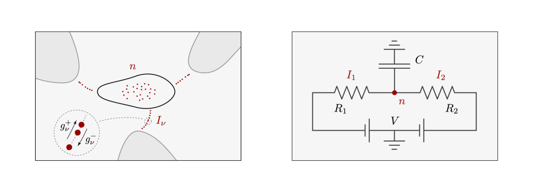
Figure 1: (Color online) Left panel: Schematic illustration of a generic system exchanging particles with $M$ reservoirs. Right panel: Realization in terms of an electric RC circuit.

Generally speaking, we are interested in the statistical properties of particle currents, $I_{\nu=1,\dots,M}$, flowing from some ‘system’ to $M$ connected ‘reservoirs’, see Fig. 1. Assuming particle number conservation, the instantaneous number of particles in the system $n$ is subject to a continuity equation, $\langle\dot{n}\rangle+\sum_{\nu}\langle I_{\nu}\rangle=0$. The system exchanges particles with the $\nu$th reservoir at time-dependent rates $g_{\nu,t}^{\pm}$, see Fig. 1. We require a detailed balance condition to hold,

$$\frac{g^{+}_{\nu,t}}{g^{-}_{\nu,t}}=e^{-\beta\kappa_{\nu,t}(n)},\quad\kappa_{\nu,t}(n)=\partial_{n}U(n)-f_{\nu,t},$$ (2)

stating that the logarithmic ratio of rates is governed by a cost function measuring the difference in ’energies’ $E_{\nu}(n)=U(n)-nf_{\nu}$ before and after a particle has entered the system through the $\nu$th terminal, $T\ln(g^{+}_{\nu}/g^{-}_{\nu})=-[E_{\nu}(n+1)-E_{\nu}(n)]$. Here, $f_{\nu}$ is a time-dependent driving force due to reservoir $\nu$, and $U(n)$ measures the system’s internal energy, where nonlinearities in $U(n)$ describe particle interactions and $\partial_{n}U(n)\equiv U(n+1)-U(n)$. The probability $P_{t}(n)$ to find $n$ particles at time $t$ is then governed by the one-step master equation VanKampen ; nazarov ; alex

$$\partial_{t}P_{t}(n)=-\hat{H}_{g}P_{t}(n),$$ (3)

with ’Hamiltonian’ $\hat{H}_{g}(n,\hat{p})=\sum_{\nu,\pm}\left(1-e^{\mp\hat{p}}\right)g^{\pm}_{\nu}(n)$, where $e^{\hat{p}}$ ($e^{-\hat{p}}$) raises (lowers) $n$ by one unit. At the initial time $t=-\tau$, the system is assumed to be in equilibrium, $f_{\nu,-\tau}=0$ and $P_{-\tau}(n)=\rho(n)=e^{-\beta(U(n)-F)}$ with free energy $F=-T\ln\sum_{n}\exp(-\beta U)$. During the time interval $[-\tau,\tau]$, the external forces $f_{\nu,t}$ then evolve according to a prescribed cyclic protocol, returning to $f_{\nu,\tau}=0$ at the final time $t=\tau$. Equations (2) and (3) describe a large spectrum of transport processes in and outside physics foot . Examples include charge transport in mesoscopic devices nazarov , molecular motors KolomeiskyFisher , chemical reaction networks SchmiedlSeifert , and evolution in biological quasispecies models MustonenLassig .

The master equation (3) deliberately emphasizes the analogy to an imaginary-time Schrödinger equation with Hamiltonian $\hat{H}_{g}$. This formal correspondence implies that the time evolution of $P_{t}(n)$ can be represented in terms of a path integral kubo ; alex . Applying a standard Trotter decomposition to the unit-normalized ’partition function’, $Z\equiv\sum_{n}P_{\tau}(n)=1$, one obtains $Z=\int D(n,p)\,e^{\int_{-\tau}^{\tau}dt\left(p\dot{n}-H_{g}(n,p)\right)}\rho(n_{-\tau})$, where the integration is over smooth paths $\{(n_{t},p_{t})\}$ and the ’momentum’ $p_{t}\in i\mathbb{R}$ conjugate to the particle number is integrated over the imaginary axis. For technical details concerning discretization and normalization issues, see also Ref. new . To extract information on the current profiles $\{I_{\nu,t}\}$, we introduce sources, $Z\to Z[\chi]$, by coupling $H_{g}$ to ’vector potentials’ (counting fields) $\chi=\{\chi_{\nu,t}\}$,

$$H_{g}(n,p)\to H_{g}(n,p,\chi)\equiv\sum_{\nu,\pm}\left(1-e^{\mp(p-i\chi_{\nu})}\right)g^{\pm}_{\nu}(n).$$

Much like in ordinary quantum mechanics, moments of the currents can then be generated by functional differentiation,

$$\langle I_{\nu_{1},t_{1}}I_{\nu_{2},t_{2}}\dots\rangle = \frac{i\delta}{\delta\chi_{\nu_{1},t_{1}}}\frac{i\delta}{\delta\chi_{\nu_{2},t_{2}}}\dots\Big{|}_{\chi=0}Z[\chi]$$

$$\Leftrightarrow Z[\chi] = \left\langle e^{-i\sum_{\nu}\int_{-\tau}^{\tau}dt\,\chi_{\nu}I_{\nu}}\right\rangle.$$ (4)

This identifies the sourceful partition function

$$Z[\chi] = \int D(n,p)\,e^{-S_{g}[n,p,\chi]}\rho(n_{-\tau}),$$ (5)

$$S_{g}[n,p,\chi] = -\int_{-\tau}^{\tau}dt\left(p\dot{n}-H_{g}(n,p,\chi)\right)$$

as generating functional. The current probability distribution function, $P[I]\equiv P[I_{1},\dots,I_{M}]$, follows by functional integration,

$$P[I]=\int D\chi\ e^{i\sum_{\nu}\int_{-\tau}^{\tau}dt\ \chi_{\nu}I_{\nu}}Z[\chi].$$ (6)

Following general principles bochkov1 , we now aim to relate the functional $Z$, describing evolution governed by rates $g=\{g_{\nu,t}\}$, to the functional $Z_{b}$ computed for time-reversed rates $(\hat{T}g)_{t}=g_{-t}$, i.e., $Z_{b}=Z\big{|}_{g\leftrightarrow\hat{T}g}$. Here we have defined a time reversal operator $\hat{T}$ acting on ’scalar’ functions $x=(n,g,f)$ as $(\hat{T}x)_{t}=x_{-t}$, while ’vectorial’ functions $v=(I,p,\chi)$ transform as $(\hat{T}v)_{t}=-v_{-t}$. Using Eq. (2), it is straightforward to verify that the action in Eq. (5) exhibits the invariance property

$$S_{g}[n,p,\chi] = S_{\hat{T}g}[\hat{T}n,\hat{T}(p-\beta\partial_{n}U),\hat{T}(\chi+i\beta f)]+$$ (7)

$$+ \beta[U(n_{\tau})-U(n_{-\tau})].$$

Inserting Eq. (7) into Eq. (5), and changing the integration variables $(n,p)\to(\hat{T}n,\hat{T}p)$, we obtain the symmetry relation $Z[\chi]=Z_{b}[\hat{T}(\chi+i\beta f)].$ Substituting this into Eq. (6), we arrive at a variant of the Crooks relation crooks ,

$$\frac{P[I]}{P_{b}[\hat{T}I]}=e^{-\beta\int_{-\tau}^{\tau}dt\,\sum_{\nu}f_{\nu}I_{\nu}},$$ (8)

where $P_{b}$ is the current probability distribution computed for time-inverted rates $\hat{T}g$. Equation (8) was first derived in Ref. bochkov1 by considering the symmetry of the operator $\hat{H}_{g}$ generating the system’s Markovian dynamics. Our present derivation has the advantage that it is based on a path integral representation. This gives us the option to explore the fluctuation statistics of currents beyond the rigorous bound imposed by Eq. (8). To elucidate this point, let us integrate Eq. (8) over $I$ and use normalization, $\int DIP_{b}[\hat{T}I]=1$, to obtain a variant of the Jarzynski relation

$$\langle X\rangle=1,\quad X=e^{\beta\int_{-\tau}^{\tau}dt\,\sum_{\nu}f_{\nu}I_{\nu}}.$$ (9)

On average, the currents $\langle I_{\nu}\rangle\sim-\beta g_{\nu}f_{\nu}$ follow the driving forces, which means that typically $X\sim e^{-2\tau\beta^{2}\sum_{\nu}g_{\nu}f_{\nu}^{2}}$ is an exponentially small quantity. The average value $\langle X\rangle=1$ is due to exceptional processes where currents fluctuate against the driving forces jarRareEvents . In this sense, $X$ acts as a selective observable filtering rare events. Note that the exponent in $X$ has a clear physical meaning: it refers to the work done on the system during the process.

Figure 2: (Color online) Fluctuations of the variable $X$, Eq. (9), in the RC circuit over 1000 simulated process runs. For $t_{V}/t_{T}=100$ (upper panel), the average $\langle X\rangle=1$ remains visible. However, for $t_{V}/t_{T}=1$ (lower panel), fluctuations dominate and conceal the unit average.

Before discussing the statistics of the variable $X$ in general terms, let us consider the example of a mesoscopic RC circuit biased by an external voltage, $f_{1/2,t}=\pm V_{t}/2$, see Fig. 1. While in earlier theoretical zon1 and experimental garnier studies, fluctuation relations for circuits of this type have been discussed for the thermal-noise dominated regime, we here consider the more general case of noise self-generated by transport out of equilibrium. The circuit’s stochastic evolution is described by the path integral (5) with $M=2$ and sequential tunneling rates nazarov ,

$$g_{\nu,t}^{\pm}(n)=\frac{1}{R_{\nu}}\frac{\pm\kappa_{\nu,t}(n)}{e^{\pm\beta\kappa_{\nu,t}(n)}-1},\quad\kappa_{\nu,t}=\partial_{n}U+(-)^{\nu}\frac{V_{t}}{2},$$ (10)

where $U(n)=\frac{e^{2}}{2C}(n-1/2)^{2}$ is the charging energy (assuming Coulomb blockade peak conditions). We have performed numerical simulations of Eq. (3) to compare with the analytical estimates described below. Assuming $R_{1}=R_{2}=R$, the dynamics is characterized by a number of time scales, including the $RC$ relaxation time $t_{RC}=RC/2$, the inverse of the mean rate at which charges enter the central island $t_{V}=R/V$, the scale at which thermal fluctuations lead to system-reservoir particle exchange, $t_{T}=R/T$, and the typical scale $t_{\gamma}$ of variation of the external voltage protocol. For $t_{V}/t_{T}\gg 1$, we are in a thermal regime where noise is of Johnson-Nyquist type and fluctuations are comparatively benign. However, the opposite shot noise regime, $t_{V}/t_{T}\lesssim 1$, is governed by much more aggressive fluctuations, as illustrated by the simulation results in Fig. 2. Figure 3 shows results for the ensuing changes in the probability distribution $P(X)$. Comparing the two profiles, one notices the massive broadening of $P(X)$ upon entering the shot-noise dominated regime. The near linearity of $P(X)$ on a double-logarithmic scale suggests a crossover to a power-law distribution. This indicates a divergence of all moments of $X$ except for the first, $\langle X^{l=1}\rangle=1$.

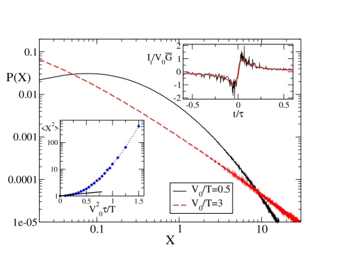
Figure 3: (Color online) Main panel: Probability distribution of $X$ in Eq. (9) obtained from $2\times 10^{6}$ simulation runs for the asymmetric voltage pulse $V_{t}=V_{0}t_{\gamma}t/(t^{2}+t_{\gamma}^{2})$, with $t_{\gamma}=0.01\tau,V_{0}\tau=250$, $\tau/t_{RC}=2\times 10^{4}$. The solid black curve ($V_{0}/T=0.5$) and the dashed red curve ($V_{0}/T=3$) probe the thermal and the near shot-noise regime, respectively. Lower inset: Simulation results for $\langle X^{2}\rangle$ vs $V_{0}^{2}\tau/T$ for $t_{\gamma}=0.01\tau,V_{0}\tau=5,\tau/t_{RC}=2\times 10^{4}$. The straight black line is a fit to Eq. (11) with $l=2$. Upper inset: The black curve gives a typical current profile for $t_{\gamma}=0.04\tau$, $V_{0}\tau=500$, $\tau/t_{RC}=2\times 10^{3}$, $\bar{G}=(2R)^{-1}$, and $V_{0}/T=10^{3}$. The red curve denotes the averaged profile.

To make these observations more quantitative, we next consider the moments $\langle X^{l\geq 1}\rangle$ within the path integral approach. While details of the discussion are adjusted to the above circuit example with $M=2$ terminals, the overall strategy is general and can readily be adapted. Equations (4) and (9) imply that $\langle X^{l}\rangle=Z[i\beta lf]$. The introduction of sources renders the minimum of the action $S_{g}[n,p,i\beta lf]$ non-vanishing. For sufficiently large observation time $2\tau$, the action is large and stationary-phase methods apply. We solve the corresponding Hamilton equations, $\dot{n}=\partial_{p}H_{g}$ and $\dot{p}=-\partial_{n}H_{g}$, under the assumption that the driving forces vary over time scales $t_{\gamma}$ larger than the intrinsic relaxation times. Again, we start from an equilibrium state and assume a cyclic force protocol, $f_{\pm\tau}=0$. Under these conditions, there exist quasistationary solutions $\dot{n},\dot{p}\simeq 0$, and the equations become algebraic. The further procedure sensitively depends on whether we are in the thermal regime defined by $\beta\tilde{f}<1$ for all times, where $\tilde{f}_{t}=|f_{1}-f_{2}|$, or in the off-equilibrium case realized otherwise.

In the thermal regime, fluctuations around the averages $\langle n\rangle$ and $\langle I_{\nu}\rangle$ are moderate, and the path integral can be expanded to second order in the variables $p+\beta lf_{\nu}$. This expansion, equivalent to the Kramers-Moyal expansion of the master equation VanKampen , reduces the path integral to the Martin-Siggia-Rose functional corresponding to the Fokker-Planck equation alex . In this regime, we may employ the high-temperature expansion of Eq. (2), $g^{\pm}_{\nu}\approx g_{\nu}(1\mp\frac{\beta\kappa_{\nu}}{2})$. While the ensuing equations, quadratic in $p$, afford straightforward solutions, details depend on the $n$-dependence of the rates. We here consider the prototypical situation of $n$-independent equilibrium rates $g_{\nu}$. It is then straightforward to show that $p=-l\beta\sum_{\nu}f_{\nu}g_{\nu}/\sum_{\nu}g_{\nu}$, while $n$ is determined implicitly by the condition $\dot{n}=-\langle I_{1}\rangle-\langle I_{2}\rangle=0\Rightarrow\sum_{\nu}g_{\nu}\kappa_{\nu}=0$. Substituting this configuration into the action, we obtain

$$\langle X^{l}\rangle\sim\exp\left[l(l-1)\beta\int dt\ \langle I\rangle\tilde{f}\right],$$ (11)

where $\langle I\rangle=-\langle I_{1}\rangle=\beta\frac{g_{1}g_{2}}{g_{1}+g_{2}}\tilde{f}$ is the average time-dependent linear-response current (we assume $f_{1}>f_{2}$).

In the nonequilibrium regime, however, the shift $\chi=i\beta lf$ represents a massive (exponential) intrusion into the action. The stationary phase equations are then solved by the optimal $p$-configuration $p=\frac{1}{2}\ln\left(\frac{\sum_{\nu}e^{-l\beta f_{\nu}}g_{\nu}^{+}}{\sum_{\nu}e^{+l\beta f_{\nu}}g_{\nu}^{-}}\right),$ while the sub-exponential action dependence on $n$ is less important. Substitution of $(n,p)$ into the action leads to a super-exponential scaling with the driving force fn_mismatch ,

$$\langle X^{l}\rangle\sim\exp\left[2\int dt\langle I\rangle\left(-1+e^{\frac{\beta}{2}(l-1)\tilde{f}}\right)\right].$$ (12)

This result shows that the moments do not diverge but become extraordinarily large upon entering the nonequilibrium regime. Once the condition $\beta\tilde{f}_{t}\ll 1$ is violated, the unit average $\langle X\rangle=1$ is completely masked and the fluctuation relation (9) looses its practical meaning.

Equations (11) and (12) exemplify how the fluctuation statistics of $X$ changes dramatically upon departing from equilibrium and how these changes contain telling information on the relevant nonequilibrium processes. For example, Eqs. (11) and (12) have been derived for the rates (10), which in turn rely on the assumption of a uniform temperature $T$ (generally established by external cooling.) In the complementary case of thermal isolation, the system will heat up by the very currents the FRs are probing. In this case, the statistics of $X$ – which should be straightforward to measure experimentally – couples to the effective particle distributions building up in the system. Comparison to analytic results may then probe the validity of models for nonequilibrium transport and the ensuing theoretical descriptions. It is in this sense that we believe the fluctuations of $X$ (and other variables entering FRs) to contain far-reaching information beyond the rigorous FRs themselves.

This work was supported by the SFB TR 12 of the DFG and by the Humboldt foundation.

References

- (1) C. Bustamante, J. Liphardt and F. Ritort, Physics Today 58, 43 (2005).
- (2) R.J. Harris and G. Schütz, J. Stat. Mech. P07020 (2007).
- (3) E.M. Sevick, R. Prabhakar, S.R. Williams, and D.J. Searles, Annu. Rev. Phys. Chem. 59, 603 (2008).
- (4) U.M.B. Marconi, A. Puglisi, L. Rondoni, and A. Vulpiani, Phys. Rep. 461, 111 (2008).
- (5) M. Esposito, U. Harbola, and S. Mukamel, Rev. Mod. Phys. 81, 1665 (2009).
- (6) C. Jarzynski, Phys. Rev. Lett. 78, 2690 (1997).
- (7) D.M. Carberry, S.R. Williams, G.M. Wang, E.M. Sevick, and D.J. Evans, J. Chem. Phys. 121, 8179 (2004); R.C. Lua and A.Y. Grosberg, J. Phys. Chem. B 109, 6805 (2005); G.E. Crooks and C. Jarzynski, Phys. Rev. E 75, 021116 (2007).
- (8) G.P. Morriss and D.J. Evans, Phys. Rev. A 37, 3605 (1988).
- (9) C. Jarzynski, Phys. Rev. E 73, 046105 (2006).
- (10) N.G. Van Kampen, Stochastic Processes in Physics and Chemistry, 3rd edition (Elsevier, Amsterdam, 2007).
- (11) Yu.V. Nazarov and Ya.M. Blanter, Quantum Transport: Introduction to Nanoscience (Cambridge University Press, Cambridge, 2009).
- (12) A. Altland and B.D. Simons, Condensed matter field theory, 2nd edition (Cambridge University Press, Cambridge, 2010).
- (13) R. Kubo, K. Matsuo, and K. Kitahara, J. Stat. Phys. 9, 51 (1973); P. Hänggi, Z. Phys. B 31, 407 (1978).
- (14) S. Pilgram, A.N. Jordan, E.V. Sukhorukov, and M. Büttiker, Phys. Rev. Lett. 90, 206801 (2003).
- (15) The generalization to reservoir-specific temperatures, several types of particles, or to multiple-step master equations is straightforward.
- (16) A. Kolomeisky and M.E. Fisher, Annu. Rev. Phys. Chem. 58, 675 (2007).
- (17) T. Schmiedl and U. Seifert, J. Chem. Phys. 126, 044101 (2007).
- (18) V. Mustonen and M. Lässig, PNAS 107, 4248 (2010).
- (19) F. Langouche, D. Roekaerts, and E. Tirapegui, Functional integration and semiclassical expansions (Reidel, Dordrecht, The Netherlands, 1982).
- (20) G.N. Bochkov and Yu.E. Kuzovlev, Zh. Eksp. Teor. Fiz. 72, 238 (1977) [Sov. Phys. JETP 45, 125 (1977)]; Zh. Eksp. Teor. Fiz. 76, 1071 (1979) [Sov. Phys. JETP 49, 543 (1979)]; Physica 106A, 443 (1981); M. Campisi, P. Talkner, and P. Hänggi, arXiv:1003.1052.
- (21) G.E. Crooks, Phys. Rev. E 60, 2721 (1999); ibid. 61, 2361 (2000). See also: M. Campisi, P. Talkner, and P. Hänggi, Phys. Rev. Lett. 102, 210401 (2009).
- (22) R. van Zon and E.G.D. Cohen, Phys. Rev. Lett. 91, 110601 (2003); R. van Zon, S. Ciliberto, and E.G.D. Cohen, ibid. 92, 130601 (2004).
- (23) N. Garnier and S. Ciliberto, Phys. Rev. E 71, 060101 (2005); S. Nakamura et al., Phys. Rev. Lett. 104, 080602 (2010); Y. Utsumi et al., Phys. Rev. B 81, 125331 (2010).
- (24) The derivation of Eq. (12) neglects terms of . Therefore the exponents in Eqs. (11) and (12) do not numerically match at borderline values .