Network–wide Statistical Modeling and Prediction of Computer Traffic

Abstract

In order to maintain consistent quality of service, computer network engineers face the task of monitoring the traffic fluctuations on the individual links making up the network. However, due to resource constraints and limited access, it is not possible to directly measure all the links. Starting with a physically interpretable probabilistic model of network–wide traffic, we demonstrate how an expensively obtained set of measurements may be used to develop a network–specific model of the traffic across the network. This model may then be used in conjunction with easily obtainable measurements to provide more accurate prediction than is possible with only the inexpensive measurements. We show that the model, once learned may be used for the same network for many different periods of traffic. Finally, we show an application of the prediction technique to create relevant control charts for detection and isolation of shifts in network traffic.

, and

t1The authors were partially funded by the NSF grant DMS–0806094.

1 Introduction and Preliminaries

Computer networks consist of nodes (routers and switches) connected by physical links (optical or copper wires). Data from one node (called a source) to another (destination) is sent over the network on predetermined paths, or routes. We will call the stream of data between a particular source/destination pair a flow. The so–called flow–level traffic may traverse only a single link, if the source and destination nodes are directly connected, or several links, if they are not. Also of interest is the aggregate data traversing each link. The traffic on a given link is the sum of the traffic of the various flows using the link.

Both the flow–level and link–level traffic have been studied in the literature. Flow level data is expensive to obtain and process, but provides information directly about the flows. Data, especially that involving packet delays from source to destination, has been used to do something. See some references. On the other hand, the link level data is less expensive to obtain, but provides less information about the underlying flows. These data have been studied extensively by the field of network tomography.

This work examines the problem of predicting the traffic level on an unobserved link via measurements on a subset of the other links in the network. Rather than focusing solely on the inexpensive link level data, we also employ flow–level measurements to inform a model that can then be utilized to make solve the prediction problem. We demonstrate that this model, although initially requiring the expensive flow–level data, may be used with a large range of link level data from the same network. Thus, this work is the first to combine both flow and link level data in an efficient and feasible way.

The remainder of the paper is laid out as follows. Section 2 discusses the computer network framework and the link–level prediction problem in detail. Section 3 describes the proposed model that utilizes the flow–level traffic. Section 4 demonstrates the robustness of the resulting model, while Section 5 illustrates a potential application of the methodologies described herein in the case when all links may be observed.

2 Network Modeling and Prediction

Here, we introduce some notation and motivate our modeling framework in the context of network prediction.

2.1 Global Traffic Modeling in Computer Networks

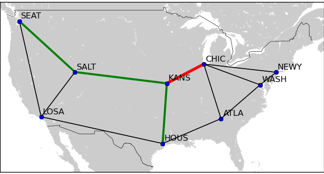
Computer networks consist of collections of nodes (routers and switches) connected by physical links (optical or copper wires). The networks may be viewed as connected directed or undirected graphs. Figure 1 illustrates, for example, the topology of the Internet2 backbone network I2 , comprised of 9 nodes (routers) and 26 unidirectional links.

Let $n$, $L$ and ${\cal J}$ denote the number of nodes, links, and routes, respectively, of a given network. Typically, every node can serve both as a source and a destination of traffic and thus there are ${\cal J}=n(n-1)$ different routes corresponding to all ordered $(source,destination)$ pairs. Computer traffic from one node to another is routed over predetermined sets of links called paths or routes. These paths are best described in terms of the routing matrix $A=(a_{\ell j})_{L\times{\cal J}}$, where

$$a_{\ell j}=\left\{\begin{array}[]{rl}1&\mbox{link $\ell$ used in route $j$}\\ 0&\mbox{link $\ell$ not used in route $j$ }\end{array}\right.\ \ \ 1\leq\ell\leq L,\ 1\leq j\leq{\cal J}.$$

The rows of the matrix $A$ correspond to the $L$ links and the columns to the ${\cal J}$ routes. In the Internet2 network, for example, the route $j$ from Chicago to Kansas City involves only one link, and thus the $j$–th column of $A$ has a single ’$1$’ on corresponding to the link connecting the two nodes; similarly, the $k$–hop routes correspond to columns of $A$ with precisely $k$ $1$’s.

Figure 1: The Internet2 topology, with prediction scenario 7 highlighted (see Table 5).

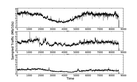
We are interested in the statistical modeling of the traffic on the entire network. Let $X(t)=(X_{j}(t))_{1\leq j\leq{\cal J}}$ be the vector of the traffic flows at time $t$ on all ${\cal J}$ routes, i.e. between all source–destination pairs. That is, $X_{j}(t),\ t=1,2,\cdots,$ is the number of bytes transmitted over route $j$ during the time interval $((t-1)h,th]$, for some fixed $h>0$. Depending on the context, the time units ($h$) can range from a few milliseconds up to several seconds or even minutes. Similarly, let $Y(t)=(Y_{\ell}(t))_{1\leq\ell\leq L}$ be the vector of the traffic loads at time $t$ over all $L$ links. Figures 2 and 3 illustrate flow– and link–level traffic over the Internet2 network.

Assuming that traffic propagates instantaneously through the network, the load $Y_{\ell}(t)$ on link $\ell$ at time $t$ equals the cumulative traffic of all routes using this link:

$$Y_{\ell}(t)=\sum_{j=1}^{\mathcal{J}}a_{\ell j}X_{j}(t)=\sum_{j\in A_{\ell}}X_{j}(t),$$

where $A_{\ell}\subset\{1,\dots,\mathcal{J}\}$ is the set of routes that involve link $\ell$. In matrix notation, we obtain

$$Y(t)=AX(t).$$ (2.1)

We shall refer to (2.1) as to the routing equation. In practice, this relationship between the flow–level traffic $X(t)$ and the link–level traffic $Y(t)$ is essentially exact, provided that the time scale of measurement $h$ is comparable or greater than the maximum round trip time (RTT) for packets in the network. In this paper, we consider aggregate data over 10 second intervals, a time substantially greater the the RTT of a packet over the Internet2 backbone.

Figure 2: Sampled traffic flow ($X_{j}(t)$) time series for high, medium, and low volume flows on the Internet2 network, recovered from NetFlow data (see Appendix 6.2, for technical details).

The statistical behavior of the network traffic traces over individual links or flows has been studied extensively in the past 20 years. An important burstiness phenomenon was observed, which rendered the classical telephone traffic models based on Poisson and Markov processes inapplicable. Mechanistic and physically interpretable models were developed that explain and relate the observed burstiness to the notions of long–range dependence and self–similarity. For more details, see eg Willinger et al. (1995), Taqqu, Willinger and Sherman (1997), Park and Willinger (2000), Mikosch et al. (2002), Stoev, Michailidis and Vaughan (2010), and the references therein.

Under general conditions, limit theorems show that the cumulative fluctuations of the traffic about its mean can be naturally modeled with fractional Brownian motions (fBm). The fBm’s are zero mean Gaussian processes, which have stationary increments and are self–similar. For more details, see Willinger et al. (2003) or Section 5 below. Other limit regimes are also possible, which lead to stable infinite variance models. These models, however, are less robust to network configurations than the fractional Brownian motion and are encountered less frequently in practice (see eg Mikosch and Samorodnitsky (2007)).

Here, our focus is not on the temporal dependence of traffic, which has been studied extensively. Rather, our goal is to model the global structural relationship between all links on the network at a fixed instant of time, $t_{0}$. Motivated by existing single–flow models, we shall suppose that the vector $X(t)$ representing the traffic on all flows of the network is multivariate normal:

$$X(t)\sim N(\mu_{X}(t),\Sigma_{X}(t)).$$ (2.2)

As discussed in Stoev, Michailidis and Vaughan (2010), the link–level, as well as flow–level traffic can be well–modeled by using multivariate long–range dependent Gaussian processes. The routing equation (2.1) yields:

$$Y(t)\sim N(A\mu_{X}(t),A\Sigma_{X}(t)A^{t}).$$ (2.3)

A first natural application and in fact our motivation to develop global network traffic models comes from the network prediction problem. The performance of our models will be explored and illustrated in this context.

Network Prediction (Kriging): Observed are the traffic traces on a subset of links ${\cal O}\subset\{1,\cdots,L\}$:

$${\cal D}(t_{0},m):=\{Y_{\ell}(t),\ t_{0}-m+1\leq t\leq t_{0},\ \ell\in{\cal O}\}.$$ (2.4)

over the time window $t_{0}-m+1\leq t\leq t_{0}$ of size $m$.

Obtain estimators $\widehat{Y}_{\ell}(t_{0})$ for the traffic $Y_{\ell}(t_{0})$, for all unobserved links $\ell\in{\cal U}:=\{1,\cdots,L\}\setminus{\cal O}$ at time $t_{0}$ in terms of the data ${\cal D}(t_{0},m)$.

In view of the Gaussianity of our global traffic model, we focus on linear predictors. In the next section, we start by adapting the classical ordinary kriging methodology from Geostatistics to the networking context. This is perhaps the best that one can do given no prior statistical information about the network other than its topology and routing. Even in such a limited setting it turns out that one can sometimes obtain useful predictors.

In many $({\cal O},{\cal U})$–scenarios, however, ordinary network kriging does not provide helpful results. The main problem is the lack of information about the traffic means (and to a lesser degree covariances) on the unobserved links. This issue can only be resolved by incorporating additional, network–specific information about the traffic. We do so, in Section 3, where by exploring (off–line) large NetFlow data sets, we recover estimates of all flows $X_{j}(t)$’s in the network. These data are used to build a flexible network–specific model that can be estimated on–line from link–level measurements. The resulting model will be shown to substantially outperform the ordinary network kriging methodology.

2.2 General Theory

If the means and covariances are known, then the network prediction problem in the previous section becomes the simple kriging problem from Spatial Statistics. The best linear unbiased predictor (BLUP) for $Y_{u}=Y_{u}(t)$ in terms of $Y_{o}=Y_{o}(t)$ is then given by:

$$\widehat{Y}_{u}={\mu}_{u}+\Sigma_{uo}\Sigma^{-1}_{oo}({Y}_{o}-{\mu}_{o}),$$ (2.5)

where

$$Y=\left(\begin{array}[]{l}Y_{o}\\ Y_{u}\end{array}\right),\ \mu_{Y}=\left(\begin{array}[]{l}\mu_{o}\\ \mu_{u}\end{array}\right),\ \mbox{ and }\ \Sigma_{Y}=\left(\begin{array}[]{ll}\Sigma_{oo}&\Sigma_{ou}\\ \Sigma_{uo}&\Sigma_{uu}\end{array}\right).$$

Here ${\mathbb{E}}Y(t)=\mu_{Y}(t)$ and $\Sigma_{Y}=\Sigma_{Y}(t)$ are the mean and the covariance matrix of the vector $Y(t)$, which is partitioned into an observed and unobserved components $Y_{o}(t)$ and $Y_{u}(t)$, respectively. For simplicity, we omit the argument ‘$t$’ in (2.5), but it is implicitly present in all quantities therein. The (conditional) covariance matrix of prediction errors $Y_{u}-\widehat{Y}_{u}$ is given by:

$${\mathbb{E}}{\Big{(}}({Y}_{u}-\widehat{Y}_{u})({Y}_{u}-\widehat{Y}_{u})^{t}|Y_{o}{\Big{)}}=\Sigma_{uu}-\Sigma_{uo}\Sigma^{-1}_{oo}\Sigma_{ou}.$$ (2.6)

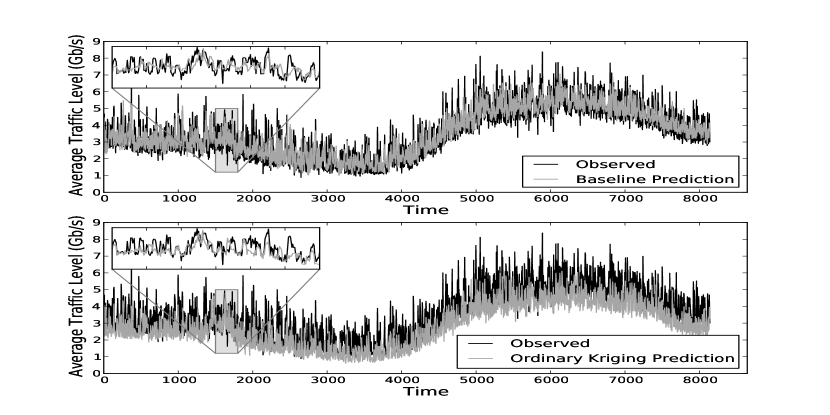
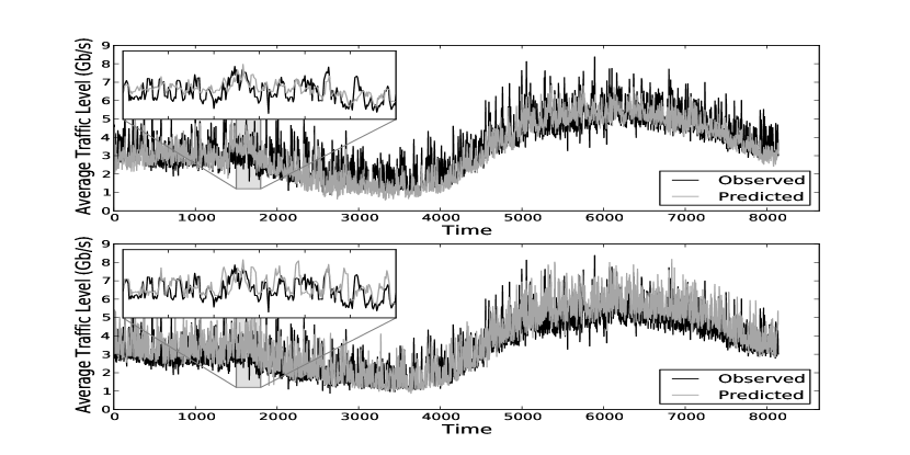
The performance of the simple kriging predictor is illustrated in Figure 3 (top), and Table 1 ($2$nd column). In these cases, $\mu_{Y}(t)$ and $\Sigma_{Y}(t)$ are estimated from moving windows of past observations, where data on all links is available (see Appendix 6.3). In the context of our network prediction problem, however, not all links are observed, the means and covariances are unknown, and the simple kriging methodology is not practical. Nevertheless, it provides a theoretically optimal benchmark that we will be used to evaluate all methods developed in the sequel.

Figure 3: Top: the standard kriging estimator based on past empirical means and covariances. This baseline estimator is not available in practice when only a subset of links is observed. Bottom: the ordinary kriging estimator. Both plots represent Scenario 7: the prediction of link 13 via links 3, 9, and 12, depicted in Figure 1.

The relative mean squared errors (ReMSE) of the predictors reported in Table 1, and in the sequel, are computed as follows:

$${\rm ReMSE}(\widehat{Y})=\sum_{t=1}^{T}\|\widehat{Y}(t)-Y(t)\|^{2}/\sum_{t=1}^{T}\|Y(t)\|^{2}.$$ (2.7)

Here $\widehat{Y}(t)$ is a predictor for the true value $Y(t)$ and $\|\cdot\|$ stands for the Euclidean norm. The ReMSE’s quantify empirically the prediction error relative to the energy of the true signal $Y(t)$, over the duration $T$. In a controlled setting where $Y(t)$ is available, the ReMSE’s allow us to objectively compare the performance of various estimators.

A first practical solution to the network prediction problem may be obtained by using the ordinary kriging methodology. Namely, suppose that we have no prior information about the statistical behavior of the traffic over the network, but the routing matrix is available. Then reasonable working assumptions are that ${\mathbb{E}}Y(t)=\mu(t)\vec{1}$ and $\Sigma_{X}(t)=\sigma_{X}^{2}(t)\mathbb{I}_{{\cal J}}$, where $\mu(t)\in\mathbb{R}$ and $\sigma_{X}(t)>0$ are unknown constant parameters, which vary slowly with time $t$. That is, the traffic means of all links are equal to $\mu(t)$, and the covariance matrix of the flow–level traffic is scalar. Using these assumptions together with the routing equation (2.1), one can obtain the best linear unbiased predictor of $Y_{u}(t)$ (see Appendix 6.3 and Cressie (1993) for more details).

Scenario	Baseline	2009-02-19	2009-02-18	2009-02-20	2009-02-26	2009-03-12
1	0.0305	0.4052	0.4212	0.4250	0.4383	0.3708
2	0.0287	0.1266	0.1194	0.1292	0.1072	0.1068
3	0.0288	0.3279	0.3315	0.3432	0.3151	0.3368
4	0.0290	0.4193	0.4342	0.4391	0.3922	0.4460
5	0.0314	0.1209	0.0807	0.0958	0.0962	0.1122
6	0.0285	1.0241	0.8644	0.9323	0.8897	0.6881
7	0.0262	0.1129	0.1225	0.1241	0.1330	0.1435
8	0.0216	0.0614	0.0585	0.0628	0.0805	0.0880
9	0.0242	0.1079	0.1011	0.1059	0.1463	0.1294
10	0.0766	12.6471	10.5816	10.2204	10.6031	10.1767
11	0.0727	0.8423	0.7394	0.6346	0.6182	0.7268
12	0.0723	0.2649	0.2338	0.2274	0.2132	0.2486

Table 1: Columns 2 and 3: ReMSE’s (see (2.7)) of the baseline (simple kriging) and ordinary kriging estimators for February 19, 2009, in 12 prediction scenarios (Tables 4 and 5). Columns 4 to 7: ReMSE’s for the ordinary kriging estimators over 4 additional days in each scenario.

Figure 3 (bottom) and Table 1 demonstrate the performance of this ordinary kriging methodology. It is certainly uniformly inferior to the benchmark estimator in Figure 3 (top) and Table 1 (column 2), which involves data on the unobserved links. Nevertheless, ordinary kriging may be useful in cases when no structural information about the network is available.

In the following section, we will develop a model that improves substantially upon the ordinary kriging methodology. This can be done, however, only by utilizing further information about the network.

3 Network Specific Modeling via NetFlow Data

3.1 Modeling Traffic Means

Direct measurements of the flow–level traffic $X(t)$ are very expensive to obtain because this would involve examining the entire traffic load of the network, i.e. storing and then processing 95–170 Gigabytes of data per day. Modern routers, however, implement a mechanism called “NetFlow”, which allow for random (Bernoulli) sampling of the flow of traversing packets. The routers store important information such as the ports, source and destination IP addresses, etc. from a sample of packet headers. Even though in fast backbone networks (eg Internet2) the practical sampling rates are eg 1 out of 100 packets, the NetFlow mechanism provides unique information about the traffic loads in the network. Using a careful mapping procedure, we assigned the sampled packets to one of the 72 source/destination flows. We thus constructed an estimate $\{\widetilde{X}(t)\}\approx\{X(t)\}$ of the flow–level traffic. Unfortunately, this method is computationally expensive to implement, which makes it impractical to use repeatedly, and it is difficult to apply in an on–line fashion. Therefore, the information derived from NetFlow can only be viewed as auxiliary data in the context of network prediction. We shall use this information to build a flexible network–specific model that can be estimated on–line.

(a) Windowed Means

(b) Energy

Figure 4: Left: The columns correspond to local sample means over consecutive windows of 2000 seconds for each of the ${\cal J}=72$ flows. Darker shades indicate higher values. The data were reconstructed from NetFlow measurements of the Internet2 network for Feb 19, 2009. Right: cumulative energy captured by the $F$ matrix for increasing values of $p$ (see (3.1) and Proposition 1 below.)

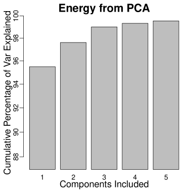
Figure 4a illustrates the local means of the source/destination flows as a function of time, where the data were derived from an extensive analysis of NetFlow measurements. This suggests that a linear model for $\mu_{X}(t)$ with a few constant factors can capture much of the variability in the local means. We therefore posit the model

$$\mu_{X}(t)=F\beta(t),$$ (3.1)

where $F$ is a suitably chosen $\mathcal{J}\times p$ matrix and $\beta=\beta(t)\in\mathbb{R}^{p}$ is a parameter. Observe that

$$\mu_{Y}=A\mu_{X}=AF\beta\ \ \mbox{ and also }\ \ \mu_{Y_{\rm o}}=A_{o}F\beta.$$

Provided $p$ equals ${\rm rank}(A_{o}F)$ the parameter $\beta$ can be successfully estimated by using linear regression from the available data on the observed links. We will see that this essentially means that $p$ is no greater than the number of observed links $|{\cal O}|$.

Now, our goal is, given $p$, to choose $F$ optimally so that $F\beta$ can approximate best $\mu_{X}$ with a suitable $\beta$. Consider the sample $\widetilde{X}(t),\ 1\leq t\leq n$, of the flow–level data derived from the NetFlow mapping, where $n=w\times n_{w}$. Partition the data into $n_{w}$ windows of size $w$, and let

$$\overline{X}(k)=\frac{1}{w}\sum_{i=1}^{w}\widetilde{X}((k-1)w+i)\$$

$(1\leq k\leq n),$ be the sample mean the $\widetilde{X}(t)$’s in the $k$–th window.

Consider first the set of $n_{w}$ points $\{\overline{X}(k),\ 1\leq k\leq n_{w}\}$ in ${\mathbb{R}}^{L}$ and observe that the model in (3.1) postulates that $\mu_{X}$ belongs to ${\rm range}(F)$ (the linear space spanned by the columns of $F$). Thus, given the $\overline{X}(k)$’s, a least squares optimal choice of $F$ corresponds to minimizing the sum of the squared distances from the $\overline{X}(k)$’s to the $p-$dimensional subspace $W:={\rm range}(F).$ That is, we want to find

$$W^{*}=\mathop{{\rm Argmin}}_{W\leq{\mathbb{R}}^{L},\ {\rm dim}(W)=p}\sum_{k=1}^{n_{w}}\|\overline{X}(k)-P_{W}(\overline{X}(k))\|^{2},$$

where $P_{W}$ denotes the orthogonal projection onto the subspace $W$. The following result shows that this problem has a simple solution, which corresponds precisely to performing principal component analysis (PCA) on a certain matrix.

Proposition 1.

Let $x(k)\in{\mathbb{R}}^{m},\ 1\leq k\leq n$. Consider the positive semidefinite $m\times m$ matrix $B=\sum_{k=1}^{n}x(k)x(k)^{t}$ and let $B=\sum_{j=1}^{m}\lambda_{j}b_{j}{b}_{j}^{t},$ be its spectral decomposition, where $b_{j},\ 1\leq j\leq m$ are orthonormal and $\lambda_{1}\geq\lambda_{2}\geq\cdots\geq\lambda_{m}\geq 0$.

Set $W^{*}={\rm span}\{{b}_{1},\dots,{b}_{p}\}$, $1\leq p\leq m$. Then, for all $W\leq{\mathbb{R}}^{m}$ with ${\rm dim}(W)=p$, we have that

$$\sum_{k=1}^{m}\|x(k)-P_{W^{*}}(x(k))\|^{2}\equiv\sum_{j=p+1}^{m}\lambda_{j}\leq\sum_{k=1}^{n}\|x(k)-P_{W}(x(k))\|^{2},$$ (3.2)

where $P_{W}$ denotes the orthogonal projection onto the subspace $W$.

The proof is given in Appendix6.4. This result implies that the least square optimal choice of the matrix $F$ is $F=({b}_{1},\cdots,{b}_{p})_{{\cal J}\times p}$, where the $b_{i}$’s, $1\leq i\leq p$ are the eigenvectors of the largest $p$ eigenvalues of the matrix $B=\sum_{k=1}^{n_{w}}\overline{X}(k)\overline{X}(k)^{t}.$ Figure 4b shows that just a few PCA factors $p$ are enough to capture a large percentage of the local variability of the mean vectors $\overline{X}(t)$. Figure 5 (top) illustrates the prediction performance of this model when the covariance matrix is known, but the unobserved means are estimated from the model.

Figure 5: Top: Prediction in Scenario 7 (Table 5 and Figure 1) using the PCA–mean model (with $p=2$) and the sample covariance matrix. In reality, the sample covariances for unobserved links are not available, and this plot merely illustrates that the model (3.1) successfully captures the structure of the means. See also Figure 3. Bottom: Prediction in Scenario 7 using the complete mean–variance model with $p=2$.

3.2 Modeling the Covariances

The physical nature of network protocols, the mechanisms of transmission, and the user behavior imply strong relationship between the means and the variances of traffic traces. This relationship was shown to be ubiquitous over different types of computer networks. In the field of network tomography, for example, the mean–variance models have been successfully used to resolve challenging identifiability questions (See eg Vardi (1996); Xi, Michailidis and Nair (2006); Lawrence et al. (2006); Singhal and Michailidis (2007)). In our context, we also encountered a strong relationship between the means and the variances of traffic flows. More precisely, by exploring the sample means $\overline{X}_{j}(t)$ and standard errors $S_{j}(t)$, calculated over a window of traffic data, we observed that

$$S_{j}(t)\approx C(\overline{X}_{j}(t))^{\gamma},\ \ 1\leq j\leq{\cal J}$$ (3.3)

with $\gamma\approx 3/4$. Namely, the standard error of a source–destination flow $X_{j}(t)$ is proportional to a power of its mean.

We estimated $\gamma$ (as a function of $t$) by performing log–linear regression of $S_{j}(t)$ versus $\overline{X}_{j}(t)$ over $j,\ 1\leq j\leq{\cal J}$. The resulting estimates remained approximately constant in $t$ and close to $3/4$ regardless of the time window used. The power–law relationship is remarkably consistent in time and the regression diagnostics $R^{2}\approx 80\%$ indicate strong agreement with the model. For more details, see Figure 7a and the discussion in Section 4.3.

Singhal and Michailidis (2007) have shown that the components of the vector of $X(t)$ are, in practice, uncorrelated or at most weakly correlated. The principal exception are pairs of forward and reverse flows, eg the Chicago–Los Angeles and Los Angeles–Chicago. This correlation is arguably due to the feedback mechanism built in the TCP protocol. Our experience with NetFlow on Internet2 (eg Fig. 2 in Stoev, Michailidis and Vaughan (2010)) and limited NS2–simulations (NS2 ) confirm that this correlation is negligible at our time scales of interest, provided that the network is not congested. The study of heavy traffic scenarios beyond the operating characteristics of the network is interesting but it is outside the scope of the present work. Therefore, in this paper we shall model $\Sigma_{X}(t)$ as a diagonal matrix.

In view of this analysis, we shall impose the following structure on the flow covariances:

$$\Sigma_{X}=\sigma^{2}\mbox{diag}(|F\beta|^{2\gamma}),$$ (3.4)

where $|a|^{2\gamma}$ denotes $(|a_{i}|^{2\gamma})_{i=1}^{\cal J},$ for $a=(a_{i})_{i=1}^{\cal J}\in\mathbb{R}^{\cal J}$, and where $\mu_{X}=F\beta$.

We will show below that the parameter $\sigma$ can be estimated on–line from link–level data ($Y_{\ell}$’s). On the other hand, $\gamma$ is a structural parameter, obtained from the off–line analysis of NetFlow data. (See Section 4.3 for more details.)

3.3 The Joint Model

Combining the mean and covariance models from the previous two sections, we obtain the following complete model:

$$Y(t)=AF\beta+\sigma A{\rm diag}(|F\beta|^{\gamma})Z(t),$$ (3.5)

where $Z(t)\sim{\mathcal{N}}(0,I_{\cal J})$ is a standard normal vector in $\mathbb{R}^{\cal J}$ and where $\beta\in\mathbb{R}^{p}$ and $\sigma>0$ are unknown parameters. In this section, we will show how this model can be estimated from on–line measurements on a limited set of observed links ${\cal O}$. We will also establish asymptotic properties of the proposed estimators.

In the framework of the Network Prediction Problem (see Section 2.1), we obtain

$$\overline{Y}_{o}(t_{0})=A_{o}F\beta+\epsilon_{\overline{Y}_{o}}(t_{0}),$$

where

$$\overline{Y}_{o}(t_{0})=\frac{1}{m}\sum_{k=0}^{m-1}Y_{o}(t_{0}-k).$$ (3.6)

To establish the covariance structure of the noise $\epsilon_{\overline{Y}_{o}}$, we introduce the mild assumption that the flow–level traffic is stationary (in practice, traffic is locally stationary on the time scales of interest) and its temporal correlation structure is the same across all routes. Namely, that ${\rm Corr}(X_{j}(t),X_{j}(t+i))=\rho(i),\ 1\leq i\leq m-1,\ (1\leq j\leq{\cal J}).$ This yields

$${\rm Corr}(Y_{\ell}(t+i),Y_{\ell}(t))=\rho(i),\ 1\leq i\leq m-1,\ \ \mbox{ for all }1\leq\ell\leq L,$$

and consequently

$$\epsilon_{\overline{Y}_{o}}(t_{0})\sim{\cal N}(0,\sigma_{m}^{2}A_{o}{\rm diag}(|F\beta|^{2\gamma})A_{o}^{t}),$$ (3.7)

where

$$\sigma_{m}^{2}=\frac{\sigma^{2}}{m}{\Big{(}}1+2\sum_{i=1}^{m-1}(1-i/m)\rho(i){\Big{)}}.$$ (3.8)

The structure of the noise variance suggests a natural iterated generalized least squares (iGLS) scheme for the estimation of $\beta$.

Algorithm: (Iterated GLS)

(i) Set $\widehat{\beta}_{1}=[(A_{o}F)^{t}A_{o}F]^{-1}(A_{o}F)^{t}\overline{Y}_{o}(t_{0})$ to be the OLS (ordinary least squares) estimate of $\beta$ and let $k:=1$.

(ii) Set

$$\widehat{\beta}_{k+1}=[(A_{o}F)^{t}G(\widehat{\beta}_{k})A_{o}F]^{-1}(A_{o}F)^{t}G(\widehat{\beta}_{k})\overline{Y}_{o}(t_{0}),$$ (3.9)

where

$$G(\beta):=[A_{o}{\rm diag}(|F\beta|^{2\gamma})A_{o}^{t}]^{-1}.$$ (3.10)

(iii) Set $k:=k+1$ and repeat step (ii). Iterate until $\|\widehat{\beta}_{k+1}-\widehat{\beta}_{k}\|$ falls below a certain “convergence” threshold.

Observe that the temporal correlation structure does not need to be estimated here since it appears only in the scalar coefficient $\sigma_{m}^{2}$ of the noise variance, which cancels in (3.9). The above iGLS scheme requires that the matrices involved in steps (i) and (ii) be invertible. The following result ensures that this is indeed the case under mild natural conditions.

Proposition 2.

Suppose that $F\beta>\vec{0}$ and let $A_{o}$ be of full row–rank. Then:

(i) The inverse $G(\beta)$ in (3.10) exists, for all $\gamma>0$.

(ii) If $A_{o}F$ is of full column–rank, then the inverses

$$\Sigma_{GLS}(\beta):=[(A_{o}F)^{t}G(\beta)A_{o}F]^{-1},$$ (3.11)

and $[(A_{o}F)^{t}A_{o}F]^{-1}$ exist and are positive definite.

The proof is given in the Appendix and the assumptions are discussed in the remarks below.

Now, if the true parameter $\beta$ is known, then as shown in Chapter 3 of Cressie (1993), the minimum variance unbiased predictor (MVUP) of $Y_{u}(t_{0})$ given the data ${\cal D}$ is the standard kriging estimate

$$\widetilde{Y}_{u}:=A_{u}F\beta+\Sigma_{uo}(\beta)\Sigma_{oo}^{-1}(\beta)(Y_{o}(t_{0})-A_{o}F\beta)=:f(\beta,Y_{o}).$$

By (2.6) and (3.5), the covariance matrix of the prediction error $Y_{u}-\widetilde{Y}_{u}$ equals:

$${\rm m.s.e.}(\widetilde{Y}_{u})=\sigma^{2}{\Big{(}}\Sigma_{uu}(\beta)-\Sigma_{uo}(\beta)\Sigma_{oo}^{-1}(\beta)\Sigma_{ou}(\beta){\Big{)}},$$ (3.12)

where

$$\Sigma(\beta)=A{\rm diag}(|F\beta|^{2\gamma})A^{t}=\left(\begin{array}[]{ll}\Sigma_{oo}(\beta)&\Sigma_{ou}(\beta)\\ \Sigma_{uo}(\beta)&\Sigma_{uu}(\beta)\end{array}\right).$$ (3.13)

In practice, consider the plug–in predictor $\widehat{Y}_{u}$, where $\widehat{\beta}$ is some estimate of $\beta$. Namely,

$$\widehat{Y}_{u}:=f(\widehat{\beta},Y_{o}).$$

Since the function $f$ is continuous, the consistency of $\widehat{\beta}$ would then imply that the plug–in predictor is a consistent estimator of the MVUP $\widetilde{Y}_{u}$. The following result establishes the strong consistency of the iterated GLS estimators $\widehat{\beta}_{k}$’s, even in the presence of long–range dependence. It also shows that the $\widehat{\beta}_{k}$’s are asymptotically equivalent to the (unavailable) GLS estimator $\widehat{\beta}_{GLS}$, provided $k\geq 2$.

Theorem 1.

Suppose that $A_{o}$ and $A_{o}F$ are of full row and column ranks, respectively, and let $F\beta>\vec{0}$. Then:

(i) For all $k\geq 1,$ we have $F\widehat{\beta}_{k}>\vec{0},a.s.$ as $m\to\infty$. Hence, the estimates $\widehat{\beta}_{k},\ k\geq 1$ are well–defined, almost surely, as $m\to\infty$.

(ii) If $\rho(\tau)\to 0,$ as $\tau\to\infty$, then for any fixed $k\geq 1$, we have

$$\widehat{\beta}_{k}\stackrel{{\scriptstyle a.s.}}{{\longrightarrow}}\beta,\ \ \mbox{ as }m\to\infty.$$ (3.14)

(iii) For all $k\geq 2$, we have that,

$$\widehat{\beta}_{k}-\widehat{\beta}_{GLS}=o_{P}(\sigma_{m}),\ \mbox{ as }m\to\infty,$$

where $\widehat{\beta}_{GLS}$ is the GLS estimate of $\beta$ in the model (3.5), and $\sigma_{m}^{2}$ is given in (3.8). Moreover, ${\rm Var}(\widehat{\beta}_{GLS})=\sigma_{m}^{2}\Sigma_{GLS}(\beta)$ with $\Sigma_{GLS}$ as in (3.11).

The proof is given in Appendix 6.4. The asymptotic variance of $\widehat{\beta}_{k},\ k\geq 2$ is discussed in the remarks below.

As mentioned above, the scale parameter $\sigma$ of the covariance structure in (3.5) is not involved in the formula for the predictors $\widehat{Y}_{u}=f(\widehat{\beta}_{k},Y_{o})$ (see eg (3.9)). The parameter $\sigma$ is involved, however, in the expression of the prediction error (3.12). Therefore, to gauge the accuracy of prediction, and to be able to use our estimators for detection of anomalies (see Section 5 below), one needs an estimate of $\sigma$.

As in the case of the ordinary kriging estimator (see (6.1) below), a natural estimate of $\sigma$ is obtained as follows:

$$\widehat{\sigma}^{2}:={\mbox{vec}(\widehat{\Sigma}_{Y_{o}})^{t}\mbox{vec}(\Sigma_{oo}(\widehat{\beta}))/\mbox{vec}(\Sigma_{oo}(\widehat{\beta}))^{t}\mbox{vec}(\Sigma_{oo}(\widehat{\beta}))},$$ (3.15)

where $\Sigma_{oo}(\beta)$ is as in (3.13), $\widehat{\Sigma}_{Y_{o}}=\widehat{\Sigma}_{Y_{o}}(t_{0})$ is the sample covariance matrix of the vector $Y_{o}$, calculated from past $m$ observations $\{Y_{o}(t_{0}-k),\ 0\leq k\leq m-1\}$, and $\widehat{\beta}$ is an estimate of $\beta$.

Proposition 3.

Assume the conditions of Theorem 1(ii). Then, with $\widehat{\beta}=\beta_{k},\ k\geq 1$, for $\widehat{\sigma}^{2}$ as in (3.15), we have $\widehat{\sigma}^{2}\stackrel{{\scriptstyle a.s.}}{{\to}}\sigma^{2}$, as $m\to\infty$.

The proof is given in the Appendix.

In the following section, we will address the estimation, validation and the applications of the complete model (3.5) by using real and simulated data. We conclude this section with a few technical comments.

Remarks:

1. The model in (3.5) is realistic only if $F\beta>\vec{0}$. In our experience, the estimates $\widehat{\beta}_{k}$ obtained from real network data always satisfy $F\widehat{\beta}_{k}>\vec{0}$. This is perhaps due to the careful (optimal) choice of the matrix $F$ discussed in Section 3.1.

2. The assumption that $A_{o}$ is of full row–rank is natural since for prediction purposes, one need not include in the set of observed links ones that are perfect linear combination of other observed links. In practice, such a redundant scenario can arise only in the trivial case when some nodes do not generate traffic.

3. The full column–rank condition on $A_{o}F$ is required for the identifiability of $\beta$. If the dimension of $\beta$ is greater than the number of observed links, then the model parameters cannot be identified (see also Section 4.3 and Figure 8a). In practice, we implement the iGLS procedure by using the Moore–Penroze generalized inverse.

4. Under the assumptions of Theorem 1, one can show that for all $k\geq 2$,

   $${\mathbb{E}}[(\widehat{\beta}_{k}-\beta)(\widehat{\beta}_{k}-\beta)^{t}1_{K}(\widehat{\beta}_{k-1})]=\sigma_{m}^{2}\Sigma_{GLS}(\beta)+o(\sigma_{m}^{2}),$$ (3.16)

   as $m\to\infty$, where $K\subset\mathbb{R}^{p}$ is an arbitrary compact set containing $\beta$ in its interior and such that $F\widetilde{\beta}>\vec{0},\ \forall\widetilde{\beta}\in K$. Thus, the variance of the estimators $\widehat{\beta}_{k},\ k\geq 2$ obtained in practice is essentially asymptotically optimal.

4 Model Validation and Calibration

In this section, we evaluate our model in the context of traffic prediction. We focus on 12 representative scenarios described in Tables 4, 5 and the Appendix 6.1, below.

4.1 Performance

Tables 1 and 2 provide ReMSE’s (2.7) for the optimal baseline estimator, the ordinary kriging estimator, and our network–specific model (with $p=2$), respectively.

Scenarios 1–9 represent situations where the observed links share sufficiently many flows with the unobserved ones and thus there is enough information for relatively accurate prediction. In all these cases, the network–specific model outperforms the more naive ordinary kriging method, with an average improvement of the ReMSE by $0.1887$ points or $18.87\%$. The difference is as high as $78\%$ and as low as $0.8\%$ in favor of the network specific model. In most cases and across different days our model yields useful predictions with ReMSE’s of about $5\%$. Note that the optimal ReMSE’s (Table 1, baseline) are about $2.5\%$ in these scenarios.

In Scenarios 10–12, however, fewer flows are shared by the observed and unobserved links and hence the accurate prediction is objectively more difficult. Note that the baseline predictor (Table 1) has over twice the ReMSE’s in these cases as compared to cases 1–9. In Scenarios 11 and 12, the ordinary kriging estimator outperforms the network specific model with differences in the ReMSE’s between $19\%$ and $105\%$. The ReMSE’s of the ordinary kriging estimator, however, are greater than $21.32\%$. In Scenario 10, our model is superior to ordinary kriging for all five days, but the large ReMSE’s indicate that neither approach is particularly useful in this case.

This initial comparison shows that the network–specific model improves significantly upon the naive ordinary kriging approach and comes close to the optimal ReMSE lower bound. This is so in the cases where the prediction problem is well–posed. Scenarios 10–12 illustrate that the accuracy of prediction has natural limitations, inherent to the routing of the network, that none of the two models can overcome.

4.2 Robustness over Time

One apparent limitation of the network specific approach is that it relies on expensive flow–level data ($X_{j}$’s) to build the matrix $F$. Surprisingly, it turns out that once the matrix $F$ is obtained from flow–level measurements during a single day, it can be successfully used to model the link–level traffic for many days in the future. That is, even though the model requires the extensive off–line analysis of NetFlow data, once it is built, it can be readily estimated on–line using only link–level data and used for several days before it has to be updated. It is remarkable that all results in Table 2 are based on a model (i.e. a matrix $F$) learned from Feb 19, 2009 flow–level data. Then, the same model was used to predict $Y_{\ell}$’s in all 12 scenarios for 5 different days. Even a month later, this model continues to outperform the ordinary kriging in the first nine scenarios. Figure 6 shows also that in only one of the $6$ scenarios therein we have an appreciable increase in the prediction ReMSE’s due perhaps to an outdated model. These results may be attributed to the fact that the structure of the traffic means across all flows in the network, although complex, is relatively constant, and is therefore well–captured by the principal components involved in the matrix $F$. The model must be updated should structural changes in the network occur.

Scenario	2009-02-19	2009-02-18	2009-02-20	2009-02-26	2009-03-12
1	0.2476	0.2342	0.2363	0.2629	0.2209
2	0.0517	0.0461	0.0550	0.0424	0.0746
3	0.0514	0.0459	0.0549	0.0425	0.0750
4	0.0521	0.0465	0.0552	0.0427	0.0740
5	0.0512	0.0696	0.0658	0.0694	0.0596
6	0.2414	0.2651	0.2864	0.3344	0.2722
7	0.0468	0.0619	0.0587	0.0684	0.0462
8	0.0388	0.0501	0.0495	0.0564	0.0384
9	0.0395	0.0510	0.0504	0.0567	0.0398
10	3.6668	3.9110	3.8143	5.0877	5.5161
11	1.0322	1.1060	1.0687	1.4335	1.7803
12	0.6277	0.7618	0.6875	0.7792	0.7449

Table 2: ReMSE’s of the network–specific model. The matrix $F$ was obtained from Feb 19, 2009 NetFlow data ($X_{j}$’s), and then used to fit the model and perform prediction based on link data ($Y_{l}$’s) for five different days.

Figure 6: ReMSE of network–specific model over time. The model was learned on Feb 19, 2009 (1). The matrix is then used to predict the previous day (2), the next day (3), a day one week later (4), and a day 4 weeks later (5). Each line corresponds to one of the first six scenarios described in Table 5.

4.3 Calibration

Applying the model to real data relies on the choice of several parameters, such as $p$, $\gamma$, and $m$, as described in Section 3. The prediction performance is remarkably robust to the choice of these parameters, as discussed in detail below.

$\bullet$ The role of $\gamma$: This parameter controls the mean/variance relationship in the model (see (3.1) and (3.4)). We observed the relationship (3.3), between the sample means $\overline{X}_{j}(t)$ and standard deviations $S_{j}(t)$’s obtained from windows of the flow–level data. The parameter $\gamma$ was estimated by using a log–linear regression of $\overline{X}_{j}(t)$ versus $S_{j}(t)$, over $j,\ 1\leq j\leq{\cal J}$. This was done for a range of window sizes and times $t$, and the estimates were found to be stable and $\widehat{\gamma}\approx 3/4$, as can be clearly seen in Figure 7a. Independently, we explored the sensitivity of the model to the choice of $\gamma$ and found that the ReMSE’s are robust to all choices $\gamma\in[0.5,2]$. See Figure 7b the effect of the choice of $\gamma$ for several of the prediction scenarios. Small values of $\gamma\approx 0.5$ lead generally to slightly better ReMSE as compared to larger $\gamma$’s. This may be due to the fact that the small powers $\gamma$ lead to a ’smoother’ covariance matrix and hence have a regularizing effect. In practice, however, we need not only accurate prediction but also adequate models for the variance, in order to have reliable estimates of the prediction error. Therefore, we recommend using $\gamma\approx 3/4$ as inferred from the data.

(a) Estimating $\gamma$

(b) Effect of $\gamma$ on Prediction

Figure 7: Left: Estimates of $\gamma$ over windows of the data (top) and their $R^{2}$ values (bottom), obtained from log–linear regression of the sample standard deviations against the means across all source–destination routes. Right: ReMSE of scenarios 1-9 for choices of $\gamma$. Note that the choice of this parameter does not significantly alter the performance of the predictor for the values tested.

$\bullet$ The role of p: The parameter $p$ equals the number of principal components (columns of the matrix $F$) used to model the traffic means in (3.1). The prediction performance is robust to the choice of $p$, provided that $p$ is less than the number of observed links used in prediction. Figure 8a shows the ReMSE’s for 3 prediction scenarios as a function of $p$. In Scenarios 6, 7, and 8 the same link is predicted via two, three, and seven other links, respectively (see Table 5). If $p$ exceeds the number of observed links, then the parameter $\beta$ in (3.5) is not identifiable, potentially resulting in poor performance. This explains the peaks in the ReMSE’s at $p=2,\ 4,$ and $7$ in Scenarios 6–8. Surprisingly, in the first two cases the ReMSE’s recover as $p$ grows, even in the presence of non–identifiability. Similar patterns are seen in the other 9 prediction scenarios (omitted, for simplicity). The performance of the model remains stable for all choices of $p$ less than the number of predictors.

In light of these results, we advocate using a relatively small value of $p$, such as $2$. While a larger value of $p$ can slightly improve prediction errors when many links are observed, having small value of $p$ allows one to fit the model in a wide variety of prediction scenarios, without sacrificing the overall performance. Recall also Figure 4b.

(a) Role of $p$

(b) Mean Window

Figure 8: Left: ReMSE of scenarios 6, 7, and 8 as a function of $p$. Performance suffers when $p$ exceeds the number of observed links, but is otherwise robust to the choice of $p$. Right: ReMSE of scenarios 1–9, as a function of window size $m$ used to estimate the means. We used $p=2$ in these cases.

$\bullet$ The role of the window size $m$: In practice, at each time point $t$, the model (3.5) is estimated from a window of past $m$ data $\{Y_{o}(t-k),\ 0\leq k\leq m-1\}$. Namely, $\beta$ is obtained by using the iGLS algorithm and $\sigma$ from (3.15) (see Section 3.3). Figure 8b illustrates the effect of the window size $m$ on the quality of prediction. Note that in all scenarios therein the prediction performance is rather robust to the choice of $m$, provided that $m\geq 10$. It is remarkable that with the exception of 2 out of the 9 shown prediction scenarios the model works well even when $m$ is less than $10$.

Recall that the scalar $\sigma$ does not affect the prediction and the ReMSE’s in Figure 8b depend only on the quality of estimation of $\beta$. The parameter $\sigma$ is involved in the prediction error. Our experiments with simulated data (not shown here, for simplicity) show that the estimates of $\sigma$ are also robust to the window size $m$.

$\bullet$ Convergence of $\widehat{\beta}_{iGLS}$: In practice, the estimates of $\widehat{\beta}_{GLS}$ stabilize after a few iterations. Here we assume the convergence criterion $\|\widehat{\beta}_{k}-\widehat{\beta}_{k+1}\|<\epsilon$, with $\epsilon=0.001$, for example. In the figures and tables, however, the algorithm was allowed to run for at least 20 iterations to be conservative.

4.4 Model Misspecification

Here, we apply our model (3.5) to simulated data that violates the assumption of stationarity. Our goal is to understand the limitations of model, when applied to network traffic with slowly changing trend. Network flows are simulated using independent fractional Gaussian noise (fGn) time series with self–similarity parameter $H=0.8$ (see Section 5.1, below). This value of $H$ is typical for several real network flows that we examined.

We compare the mean squared prediction errors in the stationary and non–stationary regimes. In the stationary case, constant means are added to the simulated fGn’s to produce realistic traffic flows with constant positive means. Non–stationary traffic traces were obtained by adding a sinusoidal trend to all simulated stationary flows. In both cases (stationary and non– stationary), link–level data was obtained from the simulated flow–level data through the routing equation (2.1).

We focused on prediction Scenario 8 (see Table 5). We computed the baseline ‘simple kriging’ predictor $\widetilde{Y}$ by using the known means and covariances of the simulated data. We also estimated our model and used it to obtain a predictor $\widehat{Y}$ of the unobserved link.

Table 3 shows the resulting prediction errors as a function of the window size used to estimate the parameter $\beta$.

The empirical error of our estimators are comparable to the optimal MSE’s for the baseline estimator. This is so even in the presence of non–stationarity. The major exception is when in the non–stationary case the window size becomes close to the half–period (50) of the sinusoidal trend. This limited experiment shows that our model adapts well and it is essentially robust to non–stationary trends provided that relatively small window sizes $m$ are used.

	Baseline	Network Specific Model
Window		5	10	25	30	50	75	100	200
Stationary	2.61	2.93	2.88	2.83	2.82	2.80	2.78	2.77	2.75
Non–Stationary	2.61	4.15	4.15	4.50	4.71	5.42	6.19	4.99	4.98

Table 3: Empirical mean squared errors for the baseline (simple kriging) predictor $\widetilde{Y}$ and the predictor $\widehat{Y}$, based on our network–specific model with $p=2$. Time series of 20,000 observations were used.

5 Statistical Detection of Anomalies

In this section, we present an application of the above methodology to the case when all links on the network are observed. In this case, for each link $\ell$, one can compare the observed $Y_{\ell}(t)$ and the predicted $\widehat{Y}_{\ell}(t)$ traffic. If statistically significant deviations are encountered, then this can serve as a flag of an anomaly or some structural change in the network traffic.

To illustrate and detect such differences, we use a modified exponentially weighted moving average (EWMA) control chart on the differences $Y_{\ell}-\widehat{Y}_{\ell}$. The latter have zero means and variances equal to the prediction error, which can be estimated from (3.12) and (3.15).

Although EWMA control charts are widely used and well–studied (see, e.g, Box, Luceno and del Carmen Paniagua-Quinones (2009)), they rely on an assumption of independent or weakly dependent (in $t$) observations. Computer network traffic is long–range dependent (LRD) and the usual variance formula used in the EWMA charts does not apply. We show next how these charts can be adjusted to account for the presence such dependence.

5.1 Control charts for long–range dependent data

Consider the EWMA with discount factor $\phi\in(0,1)$ of the time series $\{Z_{k}\}_{k\geq 0}$:

$$\widetilde{Z}_{t}:=(1-\phi)(Z_{t}+\phi Z_{t-1}+\phi^{2}Z_{t-2}+\cdots)$$ (5.1)

Letting $\lambda=1-\phi$, this moving average may be efficiently updated via $\widetilde{Z}_{t}=\lambda Z_{t}+(1-\lambda)\widetilde{Z}_{t-1}$. For independent $Z_{t}$’s, for ${\rm Var}(\widetilde{Z}_{t})=\sigma_{\widetilde{Z}}^{2}$, we have $\sigma_{\widetilde{Z}}^{2}=\frac{\lambda}{2-\lambda}\sigma_{Z}^{2}.$ When the $Z_{t}$’s are long–range dependent, however, the latter formula underestimates the variance $\sigma_{\widetilde{Z}}^{2}$, which can lead to frequent false positive alarms.

Internet traffic traces are well known to exhibit long–range dependence, which can be well–modeled by using fractional Gaussian noise (fGn) (see, eg Willinger et al. (2003)). Recall that the zero mean Gaussian time series $\{Z_{k}\}$ is said to be fGn if $Z_{k}=B_{H}(k)-B_{H}(k-1),k\geq 1$, where $\{B_{H}(t)\}_{t\geq 0}$ is a fractional Brownian motion with self–similarity parameter $H\in(0,1)$. The process $\{B_{H}(t)\}_{t\geq 0}$ is self–similar and has stationary increments. Its covariance function is

$${\mathbb{E}}B_{H}(t)B_{H}(s)=\frac{\sigma^{2}}{2}{\Big{(}}|t|^{2H}+|s|^{2H}-|t-s|^{2H}{\Big{)}},\ t,s>0,$$

where $\sigma^{2}={\mathbb{E}}B_{H}(1)^{2}=\mbox{Var}(B_{H}(1))$. Thus, the fGn $\{Z_{k}\}$ is a stationary time series with auto–covariance

$$\gamma_{H}(k)={\mathbb{E}}(Z_{k}Z_{0})=\frac{\sigma^{2}}{2}{\Big{(}}|k+1|^{2H}+|k-1|^{2H}-2k^{2H}{\Big{)}}.$$ (5.2)

For more details, see, eg Taqqu (2003).

The following result provides an expression for the variance $\sigma_{\widetilde{Z}}^{2}$ of the EWMA control chart corresponding to LRD fGn data.

Proposition 4.

For $\widetilde{Z}_{t}$ as in (5.1) with $Z_{t}$’s an fGn with self–similarity parameter $H\in(0,1)$ and variance $\sigma^{2}$, we have:

$${\rm{Var}}(\widetilde{Z}_{t})=\frac{\lambda^{2}\sigma^{2}}{C_{2}(H)^{2}}\int_{-\infty}^{\infty}\frac{2(1-\cos(\theta))|\theta|^{-2H-1}}{\lambda^{2}-2\lambda(1-\cos\theta)+2(1-\cos\theta)}d\theta,$$ (5.3)

where $C_{2}(H)^{2}:=\pi/(H\Gamma(2H)\sin(H\pi))$.

The proof is given in the Appendix. In practice, the expression in (5.3) is readily evaluated by using numerical integration.

5.2 Simulated Anomalies in Observed Network Traffic

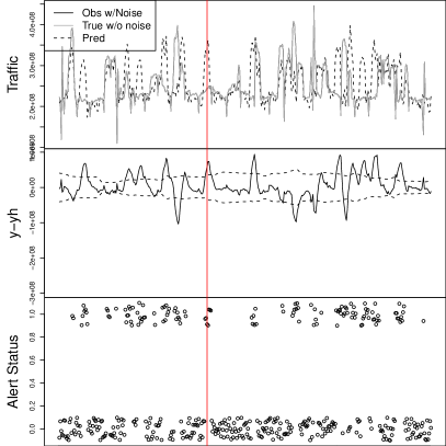
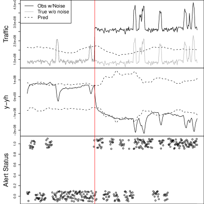
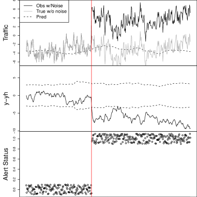
We now present some examples of using the adjusted EWMA control chart for real network data, applied to the differences $Y_{\ell}(t)-\widehat{Y}_{\ell}(t)$. The mean is taken to be $0$ for the duration of the control chart, since the predictor $\widehat{Y}_{\ell}(t)$ is unbiased under the model. The variance of the control chart is calculated using (5.3), with $\sigma^{2}$ replaced by $\widehat{\sigma}_{Y}^{2}$ (estimated in the prediction procedure). The Hurst LRD parameter $H$ of the traffic is obtained by using the wavelet–based methods described in Stoev and Taqqu (2003). In each of the examples, a simple mean–shift anomaly is added to one source–destination flow . Each figure in this section shows a plot of the observed, predicted, and true traffic (top panels); the control chart of $|Y_{\ell}-\widehat{Y}_{\ell}|$ (middle panels), and an indicator of whether the process is identified as out of control (bottom panels). The vertical line indicates the onset of the simulated anomaly.

(a) Standard EWMA Control Chart

(b) LRD–adjusted EWMA Control Chart

Figure 9: Performance of the standard EWMA control chart for i.i.d. data (left plot) and that of the LRD–adjusted chart (right plot).

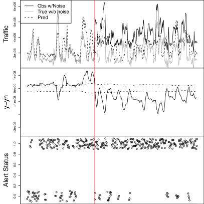
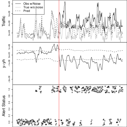
Figure 9 demonstrates the importance of the LRD–adjustment for the control limits of the EWMA charts. Here, we examine link 13 (Kansas City to Chicago), which is predicted using all links sharing at least one flow with it (Scenario 8 in Table 5). A simulated anomaly is added to flow 20, which traverses only link 13. The standard chart results in far too many false positives, making it difficult to see when the anomaly is added. While the adjusted chart still has several false positives (due to high traffic variability), the onset of the anomaly is essentially detected.

The second example shows how one can use the chart to determine which flow is behaving anomalously. The mean shift was added to flow 6 (Kansas City to Atlanta), which traverses two links: 13 (Kansas City to Chicago) and 17 (Chicago-Atlanta) (see Figure 1). The LRD–adjusted control charts for Links 13 (Figure 10a) and 17 (not shown), clearly indicate the onset of the anomaly. The charts of the other links, not carrying the anomalous flow, (eg link 7 in Figure 10b) involve just a few false alarms and detect no anomaly. This suggests that the flow using links 13 and 17 (that is, flow 6) is experiencing the anomaly.

(a) Link Carrying Anomalous Flow (13)

(b) Link Not Carrying Anomalous Flow (7)

Figure 10: Detecting an anomalous multi–link flow. The simulated anomaly is added to a two–link flow. The links carrying the flow show anomalous behavior (left plot), while the rest behave as in the figure on right.

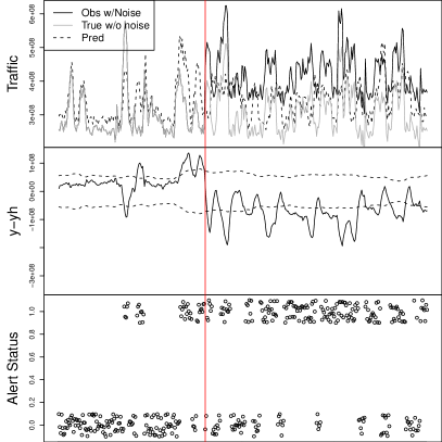
In the last example, we illustrate a case where the anomaly detection is inherently more challenging. We add a mean shift to the relatively long flow 14 (Seattle to Atlanta), which traverses four links: 3 (Seattle to Salt Lake City), 9 (Salt Lake City to Kansas City), 13 (Kansas City to Chicago), and 17 (Chicago to Atlanta) (see Figure 1). In Figure 11a, the control chart is based on predicting Link 17 by using all links that do not carry the anomalous flow. Unfortunately, these links do not provide sufficient information to predict Link 17, hence the predictor is a relatively ‘smooth curve’ as compared to the true traffic trace, and the error is relatively large. Nevertheless, we can pick up the anomaly. The segment with false positive alerts can be explained by the presence of ”bias” in our model. That is, the model $F\beta$ is not capturing the fine dynamics of the means. Indeed, if we repeat the exercise using simulated traffic (Figure 11b), it shows that again the predictor is not particularly useful i.e. it yields a smooth curve that tracks only the local means. In this situation, however, there is no bias and the control chart accurately identifies the onset of the anomaly.

(a) Real Traffic

(b) Simulated Traffic

Figure 11: An anomaly is added to flow 14 (Seattle to Atlanta), and a control chart is constructed on the Chicago–Atlanta Link (17), where all ’non–anomalous’ links are used in the prediction. These links, however, do not provide enough information and the predictor is a relatively smooth curve.

6 Appendix

6.1 Internet2 Network Description and Prediction Scenarios

Link ID	Source $\to$ Destination	Capacity
1,2	Los Angeles $\to$ Seattle	10 Gb/s
3,4	Seattle $\to$ Salt Lake City	10 Gb/s
5,6	Los Angeles $\to$ Salt Lake City	10 Gb/s
7,8	Los Angeles $\to$ Houston	10 Gb/s
9, 10	Salt Lake City $\to$ Kansas City	10 Gb/s
11, 12	Kansas City $\to$ Houston	10 Gb/s
13, 14	Kansas City $\to$ Chicago	20 Gb/s
15, 16	Houston $\to$ Atlanta	10 Gb/s
17, 18	Chicago $\to$ Atlanta	10 Gb/s
19, 20	Chicago $\to$ New York	10 Gb/s
21, 22	Chicago $\to$ Washington	10 Gb/s
23, 23	Atlanta $\to$ Washington	10 Gb/s
25, 26	Washington $\to$ New York	20 Gb/s

Table 4: ID’s of the 26 links of the Internet2 backbone. Odd Link ID’s correspond to the forward and the even to the reverse; i.e. Link 15 is the Houston to Atlanta link and Link 16 is the Atlanta to Houston link.

This appendix provides details concerning the Internet2 network, as well as the 12 prediction scenarios that were investigated earlier.

The Internet2 network consists of 26 unidirectional links. In order to simplify notation, each link was assigned an id number. Table 4 provides the mapping from the link id numbers to the source and destination of each link, as well as the link capacities at the time of data collection. At the time of the data collection, all links had a 10 Gb/s capacity, with the exception of 4 links: Chicago to Kansas City, Kansas City to Chicago, New York to Washington, and Washington to New York. These four links actually were comprised of two 10 Gb/s capacity cables, for a total capacity of 20 Gb/s. Similar upgrades have been made to other links since the data presented in this work was collected.

In the preceding analysis, estimators are compared for 12 different prediction scenarios. These scenarios are summarized in Table 5. In the scenarios, a total of three links are treated as unobserved, and a subset of the remaining links are used as predictors. The choice of these links was not entirely arbitrary. Recall that the traffic on any single link is equal to the sum of the traffic of the flows that utilize the link. The three unobserved links were chosen to represent a range in the utilization level of the links (in terms of number of flows). Link 7, predicted in scenarios 1-4, is used by a medium number of flows. Link 13, predicted in scenarios 5-9, is used by 14 flows, the most of any link. Finally, link 19 is utilized by a small number of flows.

The links used as predictors were also chosen based on the number of source/destination flows shared with the unobserved link. Namely, for each unobserved link, the predictors were selected so that they share at least one source/destination flow with the unobserved link. The exceptions are scenarios 4, 9, and 12, which involve the same set of predictors. In these three scenarios, our goal is to better understand the effect of utilization on the performance of the model.

Case	Predicted	Observed Links
1	7	2,12
2	7	2,12,13,15
3	7	2,12,13,15,23,25
4	7	2,3,9,12,15,21,23,25
5	13	3,7
6	13	3,9
7	13	3,9,12
8	13	3,7,9,12,17,19,21
9	13	2,3,9,12,15,21,23,25
10	19	3,9
11	19	3,9,13
12	19	2,3,9,12,15,21,23,25

Table 5: Description of 12 Scenarios (cases) used to evaluate the model. The choice of predictors is based on the number of shared traffic flows. The link id’s are given in Table 4.

6.2 Constructing Sampled Flow–Level Data

In this section, we briefly describe how the $X$ traffic series were created from NetFlow data. Rather than provide a complete technical description, we seek to provide intuition for how the data were constructed. NetFlow records consist of individual records, each that group a sequence of packets sharing several common characteristics including: source and destination IP address, protocol, source and destination port, and type of service. These records also include as the number of packets, number of bytes, the start, and end time of the group. The input and output interfaces were of particular importance in the mapping procedure, since they allow us to identify, for each record, the physical address from where that stream of packets arrived at the router, and the physical address of the next step on the network. In particular, it allows one to determine whether or not the series of packets arrived from the Internet2 backbone and whether it was sent out on the backbone, or to a different network. In the first pass over the data, we create a careful mapping from each (source IP, destination IP) pair to a (Source Router, Destination Router) pair. Then we pass through the data a second time, using our mapping to assign each observed flow to Source Router and Destination Router, and thereby assign each observed packet to one of the 72 source/destination flows present on the backbone.

6.3 On the implementation of simple and ordinary kriging

The baseline estimator in Section 2.2 is essentially the simple kriging predictor, which assumes knowledge of the mean and covariance of $Y$ ($\mu_{Y}(t)$ and $\Sigma_{Y}(t)$). In practice, we estimate these quantities from moving windows of past data: $\mu_{Y}(t)\approx\widehat{\mu}_{Y}(t):=\frac{1}{m}\sum_{j=1}^{m}Y(t-j)$ and

$$\Sigma_{Y}(t)\approx\widehat{\Sigma}_{Y}(t):=\frac{1}{m-1}\sum_{j=1}^{m}(Y(t-j)-\widehat{\mu}_{Y}(t))(Y(t-j)-\widehat{\mu}_{Y}(t))^{t}.$$

The ordinary kriging methodology is used in our first solution of the prediction problem in Section 2.2. In this case, $\Sigma_{Y}$ is modeled by $\sigma_{X}^{2}AA^{t}$, where the scale $\sigma_{X}$ is unknown. The means ${\mathbb{E}}Y_{\ell}=\mu_{Y}$ are unknown but assumed to be constant across the links $1\leq\ell\leq L$. Here $\sigma_{X}$ and $\mu_{Y}$ are allowed to vary slowly with time $t$. In contract, to the baseline estimator, we can no longer use $\widehat{\mu}_{Y}(t)$ and $\widehat{\Sigma}_{Y}(t)$ above since only some links are observed. Under these assumptions, the least squares optimal linear predictor of a link $Y_{u}(t)$ from $Y_{o}(t)$ becomes

$$\widehat{Y}_{u}(t)=\Lambda Y_{o}(t),\ \mbox{ where }\ \Lambda=\left(\begin{array}[]{ll}\Gamma_{oo}&\vec{1}\\ \vec{1}^{t}&0\end{array}\right)^{-1}\vec{\gamma}_{ou},$$

where $\Gamma_{oo}=({\mathbb{E}}(Y_{\ell_{i}}-Y_{\ell_{j}})^{2})_{\ell_{i},\ell_{j}\in{\cal O}}$ is a matrix of the variograms for the set of observed links ${\cal O}$ and $\vec{\gamma}_{ou}=({\mathbb{E}}(Y_{u}-Y_{\ell})^{2})_{\ell\in{\cal O}}$ is a vector of cross–variograms between the unobserved link and observed links. For more details, see Cressie (1993). The resulting ordinary kriging coefficients are such that $\vec{1}^{t}\Lambda=1$ so that the predictor is unbiased. In our application, we calculated the variograms by estimating the unknown parameter $\sigma_{X}$ from a window of past data from the observed links $Y_{o}(t)$. Namely, since $\Sigma_{Y_{o}}=\sigma_{X}^{2}A_{o}A_{o}^{t},$ we obtain the linear regression estimate

$$\widehat{\sigma}_{X}^{2}=[\mbox{vec}(A_{o}A_{o}^{t})^{t}\mbox{vec}(A_{o}A_{o}^{t})]^{-1}\mbox{vec}(\widehat{\Sigma}_{Y_{o}})^{t}\mbox{vec}(A_{o}A_{o}^{t}),$$ (6.1)

where $\mbox{vec}(B)$ stands for the vectorized matrix $B$. The estimator $\widehat{\sigma}_{X}^{2}$ corresponds to minimizing $\|\mbox{vec}(\widehat{\Sigma}_{Y_{o}})-\sigma^{2}\mbox{vec}(A_{o}A_{o}^{t})\|$ with respect to $\sigma^{2}$.

6.4 Proofs

Proof of Proposition 1.

Let $W={\rm span}\{\vec{f}_{1},\cdots,\vec{f}_{p}\}$, where $\{\vec{f}_{1},\cdots,\vec{f}_{m}\}$ is an orthonormal basis of ${\mathbb{R}}^{m}$. Observe that, for all $1\leq k\leq n$:

$$\|x(k)-P_{W}(x(k))\|^{2}=\sum_{j=p+1}^{m}\langle x(k),\vec{f}_{j}\rangle^{2}=\sum_{j=p+1}^{m}\vec{f}_{j}^{t}(x(k)x(k)^{t})\vec{f}_{j}.$$

Now, by summing over $w$, we have that the right–hand side of (3.2) equals:

$$\sum_{j=p+1}^{m}\vec{f}_{j}^{t}{\Big{(}}\sum_{k=1}^{n}x(k)x(k)^{t}{\Big{)}}\vec{f}_{j}=\sum_{j=p+1}^{m}\vec{f}_{j}^{t}B\vec{f}_{j}.$$

Clearly, the last sum is minimized when ${\rm span}\{\vec{f}_{p+1},\cdots,\vec{f}_{m}\}=(W^{*})^{\perp}\equiv{\rm span}\{\vec{b}_{p+1},\cdots,\vec{b}_{m}\}$. In this case, this sum equals $\sum_{j=p+1}^{m}\lambda_{j}$. ∎

Proof of Proposition 2.

Since $F\beta>\vec{0}$, the matrix ${\rm diag}(|F\beta|^{2\gamma})$ is positive definite. Thus, the fact that $A_{o}$ is of full row–rank, implies that the square matrix $A_{o}{\rm diag}(|F\beta|^{2\gamma})A_{o}^{t}$ is of full row–rank and hence invertible. This proves (i).

To show (ii), let $x\in\mathbb{R}^{p}$ and suppose that $x^{t}(A_{o}F)^{t}G(\beta)A_{o}Fx=0$. Thus, for the vector $y=A_{o}Fx$, we have $y^{t}G(\beta)y=0$. This, since $G(\beta)$ is positive definite, implies that $y=A_{o}Fx=\vec{0}$, which in turn yields $x=\vec{0}$, because $A_{o}F$ has a trivial null–space. We have thus shown that $(A_{o}F)^{t}G(\beta)A_{o}F$ is a positive definite matrix. ∎

Proof of Theorem 1.

Note that

$$\overline{Y}_{o}(t_{0})=A_{o}F\beta+\sigma A_{o}{\rm diag}(|F\beta|^{\gamma})\overline{Z}(t_{0}),$$

where $\overline{Z}(t_{0})=\frac{1}{m}\sum_{t=t_{0}-m+1}^{t_{0}}Z(t).$ Since $\rho(\tau)\to 0,\ \tau\to\infty$, the Maruyama’s Theorem implies that the Gaussian process $Z=\{Z(t)\}_{t\in\mathbb{Z}}$ is mixing. Therefore, $\overline{Z}(t_{0})\stackrel{{\scriptstyle a.s.}}{{\to}}0,$ and hence $\overline{Y}_{o}(t_{0})\stackrel{{\scriptstyle a.s.}}{{\to}}A_{o}F\beta,$ as $m\to\infty$.

Note that the OLS estimator $\widehat{\beta}_{1}$ is well–defined since $A_{o}F$ is of full column rank. Observe also that, since $\overline{Y}_{o}(t_{0})\stackrel{{\scriptstyle a.s.}}{{\to}}A_{o}F\beta$, we have

$$\widehat{\beta}_{1}-\beta=[(A_{o}F)^{t}A_{o}F]^{-1}(A_{o}F)^{t}(\overline{Y}_{o}(t_{0})-A_{o}F\beta)\stackrel{{\scriptstyle{\rm a.s.}}}{{\longrightarrow}}0,\ \mbox{ as }m\to\infty.$$

We proceed by induction. Let $k\geq 2$ and $\widehat{\beta}_{k-1}\stackrel{{\scriptstyle a.s.}}{{\to}}\beta,\ m\to\infty$. Then, since $F\beta>\vec{0}$, by continuity, $F\widehat{\beta}_{k-1}>\vec{0}$, almost surely, as $m\to\infty$, and $\widehat{\beta}_{k}$ is well–defined, as $w\to\infty$ (Proposition 2). Further, for all $k\geq 2$, by (3.9),

$$\widehat{\beta}_{k}=C(\widehat{\beta}_{k-1})\overline{Y}_{o}(t_{0}),$$ (6.2)

with the matrix

$$C(\widetilde{\beta}):=[(A_{o}F)^{t}G(\widetilde{\beta})A_{o}F]^{-1}(A_{o}F)^{t}G(\widetilde{\beta}).$$ (6.3)

Note that $C(\widetilde{\beta})$ is well–defined and continuous for $F\widetilde{\beta}>\vec{0}$. Since, also $C(\beta)A_{o}F\beta=\beta$, the convergences $\overline{Y}_{o}(t_{0})\stackrel{{\scriptstyle a.s.}}{{\to}}A_{o}F\beta$, and $\widehat{\beta}_{k-1}\stackrel{{\scriptstyle a.s.}}{{\to}}\beta,$ imply that $\widehat{\beta}_{k}\stackrel{{\scriptstyle a.s.}}{{\to}}\beta$, as $m\to\infty$. We have thus shown parts (i) and (ii).

We shall now prove (iii). As in (6.2), for all $k\geq 2$, we have

$$\widehat{\beta}_{k}=C(\widehat{\beta}_{k-1})\overline{Y}_{o}(t_{0})\ \mbox{ and also }\ \widehat{\beta}_{GLS}=C(\beta)\overline{Y}_{o}(t_{0}).$$

Note also that $C(\beta)A_{o}F\beta=\beta=C(\widehat{\beta}_{k})A_{o}F\beta$, and therefore,

$$\widehat{\beta}_{k}-\widehat{\beta}_{GLS}=(C(\widehat{\beta}_{k-1})-C(\beta))(\overline{Y}_{o}(t_{0})-A_{o}F\beta).$$ (6.4)

Now, by (3.7) and (3.10), we have

$${\rm Var}(\overline{Y}_{o}(t_{0}))=\sigma_{m}^{2}G(\beta)^{-1}.$$ (6.5)

Thus, Relation (6.4), the convergence $\widehat{\beta}_{k-1}\stackrel{{\scriptstyle a.s.}}{{\to}}\beta,\ m\to\infty$, and the continuity of $C(\cdot)$ imply that $\widehat{\beta}_{k}=\widehat{\beta}_{GLS}=o_{P}(\sigma_{m}),\ m\to\infty$. Note also that by (6.3) and (6.5), we readily have ${\rm Var}(\widehat{\beta}_{GLS})=\sigma_{m}^{2}\Sigma_{GLS}(\beta)$. ∎

Proof of Proposition 3.

As in the proof of Theorem 1, the Maruyama’s theorem implies that $\widehat{\Sigma}_{Y_{o}}\stackrel{{\scriptstyle a.s.}}{{\to}}\Sigma_{Y_{o}},$ as $m\to\infty.$ By Theorem 1 (ii) we also have $\widehat{\beta}_{k}\stackrel{{\scriptstyle a.s.}}{{\to}}\beta,$ as $m\to\infty$. Note that the right–hand side of (3.15) is a continuous function of $\widehat{\beta}$ and $\widehat{\Sigma}_{Y_{o}}$, which by (3.5), equals $\sigma^{2}$ when $\widehat{\beta}$ and $\widehat{\Sigma}_{Y_{o}}$ are replaced by $\beta$ and $\Sigma_{Y_{o}}$, respectively. This implies the strong consistency of $\widehat{\sigma}^{2}$. ∎

Proof of Proposition 4.

The variance of $\widetilde{Z}_{t}$ is then given by:

$${\mathbb{E}}[\widetilde{Z}_{t}^{2}]=(1-\phi)^{2}\sum_{j=0}^{\infty}\sum_{k=0}^{\infty}\phi^{j+k}\gamma(j-k)=(1-\phi)^{2}\sum_{j=0}^{\infty}\sum_{k=0}^{\infty}\phi^{j+k}\int_{-\pi}^{\pi}e^{i\theta(k-j)}f(\theta)d\theta,$$

where $f(\theta)$ stands for the spectral density of $\{Z_{k}\}$. By using the expression of $f$ given in equation 9.12 on p.34 of Taqqu (2003) , we obtain that ${\mathbb{E}}[\widetilde{Z}_{t}^{2}]$ equals

$$\lambda^{2}\int_{-\pi}^{\pi}{\Big{|}}\sum_{k=0}^{\infty}\phi^{k}e^{i\theta k}{\Big{|}}^{2}f(\theta)d\theta=\lambda^{2}C_{2}(H)^{-2}\int_{-\infty}^{\infty}\frac{2(1-\cos(\theta))|\theta|^{-(2H+1)}}{\phi^{2}+1-2\phi\cos\theta}d\theta$$

$$\ \ =\lambda^{2}C_{2}(H)^{-2}\int_{-\infty}^{\infty}\frac{2(1-\cos(\theta))|\theta|^{-(2H+1)}}{\lambda^{2}-2\lambda(1-\cos\theta)+2(1-\cos\theta)}d\theta.$$

∎

References

- Box, Luceno and del Carmen Paniagua-Quinones (2009) {bbook}[author] \bauthor\bsnmBox, \bfnmGeorge E.P.\binitsG. E., \bauthor\bsnmLuceno, \bfnmAlberto\binitsA. and \bauthor\bparticledel \bsnmCarmen Paniagua-Quinones, \bfnmMaria\binitsM. (\byear2009). \btitleStatistical Control by Monitoring and Adjustment, \beditionSecond ed. \bpublisherWiley. \endbibitem
- Cressie (1993) {bbook}[author] \bauthor\bsnmCressie, \bfnmN.\binitsN. (\byear1993). \btitleStatistics for Spatial Data: revised ed. \bpublisherJohn Wiley, \baddressNew York. \endbibitem
- (3) {bmisc}[author] \bauthor\bsnmI2, \btitleAbout Internet2. \bhowpublishedhttp://www.internet2.edu/about. \endbibitem
- Lawrence et al. (2006) {bincollection}[author] \bauthor\bsnmLawrence, \bfnmEarl\binitsE., \bauthor\bsnmMichailidis, \bfnmGeorge\binitsG., \bauthor\bsnmNair, \bfnmVijayan N.\binitsV. N. and \bauthor\bsnmXi, \bfnmBowei\binitsB. (\byear2006). \btitleNetwork tomography: a review and recent developments. In \bbooktitleFrontiers in statistics \bpages345–366. \bpublisherImp. Coll. Press, \baddressLondon. \bmrnumberMR2326009 \endbibitem
- Mikosch and Samorodnitsky (2007) {barticle}[author] \bauthor\bsnmMikosch, \bfnmThomas\binitsT. and \bauthor\bsnmSamorodnitsky, \bfnmGennady\binitsG. (\byear2007). \btitleScaling limits for cumulative input processes. \bjournalMath. Oper. Res. \bvolume32 \bpages890–918. \bmrnumberMR2363203 (2008m:60189) \endbibitem
- Mikosch et al. (2002) {barticle}[author] \bauthor\bsnmMikosch, \bfnmT.\binitsT., \bauthor\bsnmResnick, \bfnmS.\binitsS., \bauthor\bsnmRootzén, \bfnmH.\binitsH. and \bauthor\bsnmStegeman, \bfnmA.\binitsA. (\byear2002). \btitleIs network traffic approximated by stable Lévy motion or fractional Brownian motion? \bjournalThe Annals of Applied Probability \bvolume12 \bpages23–68. \endbibitem
- (7) {bmisc}[author] \bauthor\bsnmNS2, \btitleThe Network Simulator – NS2. \bhowpublishedhttp://www.isi.edu/nsnam/ns/. \endbibitem
- Park and Willinger (2000) {bincollection}[author] \bauthor\bsnmPark, \bfnmK.\binitsK. and \bauthor\bsnmWillinger, \bfnmW.\binitsW. (\byear2000). \btitleSelf-Similar Network Traffic and Performance Evaluation. In \bbooktitleSelf-Similar Network Traffic: An Overview (\beditor\bfnmK.\binitsK. \bsnmPark and \beditor\bfnmW.\binitsW. \bsnmWillinger, eds.) \bpublisherJ. Wiley & Sons, Inc., \baddressNew York. \endbibitem
- Singhal and Michailidis (2007) {barticle}[author] \bauthor\bsnmSinghal, \bfnmH.\binitsH. and \bauthor\bsnmMichailidis, \bfnmG.\binitsG. (\byear2007). \btitleIdentifiability of flow distributions from link measurements with applications to computer networks. \bjournalInverse Problems \bvolume23 \bpages1821–1850. \endbibitem
- Stoev, Michailidis and Vaughan (2010) {bincollection}[author] \bauthor\bsnmStoev, \bfnmS.\binitsS., \bauthor\bsnmMichailidis, \bfnmG.\binitsG. and \bauthor\bsnmVaughan, \bfnmJ.\binitsJ. (\byear2010). \btitleGlobal Modeling of Backbone Network Traffic. In \bbooktitleINFOCOM: The 29th Conference on Computer Communications. \endbibitem
- Stoev and Taqqu (2003) {binproceedings}[author] \bauthor\bsnmStoev, \bfnmS.\binitsS. and \bauthor\bsnmTaqqu, \bfnmM. S.\binitsM. S. (\byear2003). \btitleWavelet estimation for the Hurst parameter in stable processes. In \bbooktitleProcesses with Long-Range Correlations: Theory and Applications (\beditor\bfnmGovindan\binitsG. \bsnmRangarajan and \beditor\bfnmMingzhou\binitsM. \bsnmDing, eds.) \bpages61–87. \bpublisherSpringer Verlag, \baddressBerlin. \bnoteLecture Notes in Physics 621. \endbibitem
- Taqqu (2003) {bincollection}[author] \bauthor\bsnmTaqqu, \bfnmM. S.\binitsM. S. (\byear2003). \btitleFractional Brownian motion and long-range dependence. In \bbooktitleTheory and Applications of Long-range Dependence (\beditor\bfnmP.\binitsP. \bsnmDoukhan, \beditor\bfnmG.\binitsG. \bsnmOppenheim and \beditor\bfnmM. S.\binitsM. S. \bsnmTaqqu, eds.) \bpages5–38. \bpublisherBirkhäuser. \endbibitem
- Taqqu, Willinger and Sherman (1997) {barticle}[author] \bauthor\bsnmTaqqu, \bfnmM. S.\binitsM. S., \bauthor\bsnmWillinger, \bfnmW.\binitsW. and \bauthor\bsnmSherman, \bfnmR.\binitsR. (\byear1997). \btitleProof of a fundamental result in self-similar traffic modeling. \bjournalComputer Communications Review \bvolume27 \bpages5–23. \endbibitem
- Vardi (1996) {barticle}[author] \bauthor\bsnmVardi, \bfnmY.\binitsY. (\byear1996). \btitleNetwork tomography: estimating source-destination traffic intensities from link data. \bjournalJ. Amer. Statist. Assoc. \bvolume91 \bpages365–377. \bmrnumberMR1394093 (97a:62050) \endbibitem
- Willinger et al. (1995) {barticle}[author] \bauthor\bsnmWillinger, \bfnmW.\binitsW., \bauthor\bsnmTaqqu, \bfnmM. S.\binitsM. S., \bauthor\bsnmLeland, \bfnmW. E.\binitsW. E. and \bauthor\bsnmWilson, \bfnmV.\binitsV. (\byear1995). \btitleSelf-Similarity in high-speed packet traffic: analysis and modeling of Ethernet traffic measurements. \bjournalStatistical Science \bvolume10 \bpages67–85. \endbibitem
- Willinger et al. (2003) {bincollection}[author] \bauthor\bsnmWillinger, \bfnmW.\binitsW., \bauthor\bsnmPaxson, \bfnmV.\binitsV., \bauthor\bsnmRiedi, \bfnmR. H.\binitsR. H. and \bauthor\bsnmTaqqu, \bfnmM. S.\binitsM. S. (\byear2003). \btitleLong-range dependence and data network traffic. In \bbooktitleTheory and Applications of Long-range Dependence (\beditor\bfnmP.\binitsP. \bsnmDoukhan, \beditor\bfnmG.\binitsG. \bsnmOppenheim and \beditor\bfnmM. S.\binitsM. S. \bsnmTaqqu, eds.) \bpages373–407. \bpublisherBirkhäuser. \endbibitem
- Xi, Michailidis and Nair (2006) {barticle}[author] \bauthor\bsnmXi, \bfnmBowei\binitsB., \bauthor\bsnmMichailidis, \bfnmGeorge\binitsG. and \bauthor\bsnmNair, \bfnmVijayan N.\binitsV. N. (\byear2006). \btitleEstimating network loss rates using active tomography. \bjournalJ. Amer. Statist. Assoc. \bvolume101 \bpages1430–1448. \bmrnumberMR2279470 \endbibitem