On the temporal evolution of the stellar mass function in Galactic clusters

Abstract

We show that we can obtain a good fit to the present day stellar mass functions (MFs) of a large sample of young and old Galactic clusters in the range $0.1-10$ M_⊙ with a tapered power law distribution function with an exponential truncation of the form $dN/dm\propto m^{\alpha}\,[1-e^{-(m/m_{c})^{\beta}}]$. The average value of the power-law index $\alpha$ is $\sim-2$, that of $\beta$ is $\sim 2.5$, whereas the characteristic mass $m_{c}$ is in the range $0.1-0.8$ M_⊙ and does not seem to vary in any systematic way with the present cluster parameters such as metal abundance, total cluster mass or central concentration. However, $m_{c}$ shows a remarkable correlation with the dynamical age of the cluster, namely $m_{c}/M_{\odot}\simeq 0.15+0.5\times\tau_{\rm dyn}^{3/4}$, where $\tau_{\rm dyn}$ is the dynamical age taken as the ratio of cluster age and dissolution time. The small scatter seen around this correlation is consistent with the uncertainties on the estimated value of $\tau_{\rm dyn}$. We attribute the observed trend to the onset of mass segregation via two-body relaxation in a tidal environment, causing the preferential loss of low-mass stars from the cluster and hence a drift of the characteristic mass $m_{c}$ towards higher values. If dynamical evolution is indeed at the origin of the observed trend, it would seem plausible that high-concentration globular clusters, now with median $m_{c}\simeq 0.33$ M_⊙, were born with a stellar MF very similar to that measured today in the youngest Galactic clusters and with a value of $m_{c}\simeq 0.15$ M_⊙. This hypothesis is consistent with the absence of a turn-over in the MF of the Galactic bulge down to the observational limit at $\sim 0.2$ M_⊙ and, if correct, it would carry the implication that the characteristic mass is not set by the thermal Jeans mass of the cloud.

1. Introduction

There is general consensus that stars do not form in isolation but rather from the fragmentation of molecular clouds that leads to star clusters (e.g. Lada & Lada 2003; Elmegreen 2010). This makes stellar clusters ideal places to study the properties of star formation and its outcome, the stellar initial mass function (IMF). However, it is also equally well established today that a large majority of stars, in our Galaxy and elsewhere, are not in clusters but in the field, since clusters disrupt over time (see e.g. Gieles 2010). Therefore, any attempt to set constraints on the star formation mechanisms from the analysis of the present day stellar mass function (MF) of but the youngest clusters cannot ignore the consequences of their dynamical evolution.

This issue becomes particularly important if we want to compare the results of star formation in physically different environments and with various ages. The obvious example is addressing differences in the way low-mass stars ($<1$ M_⊙) formed in globular clusters (GCs), at $z\simeq 5$ or about 12 Gyr ago, and in young clusters (YCs) in the local universe. While in both cases the raw data show a broad plateau in the mass distribution, suggesting a characteristic mass of order a few tenths of M_⊙ (e.g. Elmegreen et al. 2008), until the effects of dynamical evolution are properly understood, no meaningful conclusion can be drawn either on the uniformity of the star formation process over time or on the possible role of the environment. In order to cover a wide range of metallicities and initial densities one is forced to compare stellar systems that formed a Hubble time apart, such as the YCs and GCs mentioned above. Therefore, the universality of the IMF over time and location remains as yet an unresolved issue.

On the other hand, even though the two-body relaxation process that governs the cluster’s dynamical evolution and that leads to preferential loss of low-mass stars is today rather well understood (e.g. Spitzer 1987), it is in general not possible to roll back the effects of dynamics and derive the IMF from the present day MF, since we cannot trace back the trajectories of stars that have escaped the cluster. It is however possible and statistically meaningful to study the evolution of the stellar MF on a global scale by looking at the differences between clusters at different evolutionary stages. This requires a homogeneous sample of high quality observations of Galactic (open and globular) clusters, treated in a uniform way and with reliable errors. Early in this decade, this type of homogeneous study became possible for GCs (Paresce & De Marchi 2000), mostly thanks to the Hubble Space Telescope. In the meanwhile, high quality data have become available for YCs as well, mostly from wide field ground based surveys, thereby making this study possible on a global scale.

Table 1The sample of stellar clusters used in this study

ID	Name	$\alpha$	$\beta$	$m_{c}$	$m$ range	$[Fe/H]$	$\log M_{\rm tot}$	$c$	$\log t$	$\log t_{\rm dis}$	$\tau_{\rm dyn}$	Ref
				[M⊙]	[M⊙]		[M⊙]		[yr]	[yr]
1	$\rho$ Oph	$-1.9\pm 0.2$	$1.9\pm 0.2$	$0.17\pm 0.03$	$0.02$ – $7$	$0.08$	$3.3$		$5.7$	$8.7$	$0.001$	a
2	Orion N. C.	$-1.9\pm 0.2$	$2.0\pm 0.3$	$0.19\pm 0.05$	$0.02$ – $50$	$-0.01$	$1.8$	$0.3$	$6.0$	$8.7$	$0.002$	b, c
3	Taurus	$-2.3\pm 0.2$	$1.8\pm 0.2$	$0.51\pm 0.05$	$0.03$ – $3.5$	$-0.03$	$1.7$		$6.0$	$6.3$	$0.5$	d
4	IC 348	$-1.9\pm 0.1$	$3.3\pm 0.2$	$0.12\pm 0.05$	$0.03$ – $2.2$	$-0.01$	$1.8$	$0.3$	$6.3$	$8.7$	$0.004$	e
5	$\sigma$ Ori	$-2.0\pm 0.1$	$3.2\pm 0.2$	$0.14\pm 0.02$	$0.02$ – $2.4$	$-0.01$	$2.3$	$0.6$	$6.5$	$8.7$	$0.006$	f
6	$\lambda$ Ori	$-1.9\pm 0.1$	$2.3\pm 0.2$	$0.12\pm 0.02$	$0.04$ – $2.7$	$-0.01$	$2.8$	$0.6$	$6.7$	$8.7$	$0.01$	g
7	Cha I	$-1.9\pm 0.2$	$2.3\pm 0.3$	$0.15\pm 0.03$	$0.01$ – $3.5$	$-0.11$	$2.6$		$6.7$	$8.7$	$0.01$	h
8	IC 2391	$-2.1\pm 0.1$	$2.4\pm 0.3$	$0.14\pm 0.02$	$0.05$ – $0.5$	$-0.09$	$2.2$	$0.6$	$7.7$	$8.8$	$0.06$	i
9	Blanco 1	$-1.7\pm 0.1$	$1.8\pm 0.2$	$0.22\pm 0.03$	$0.05$ – $1.75$	$0.14$	$3.5$	$0.6$	$8.1$	$9.1$	$0.09$	j
10	Pleiades	$-2.2\pm 0.1$	$2.3\pm 0.2$	$0.27\pm 0.03$	$0.04$ – $9$	$0.03$	$2.9$	$0.6$	$8.1$	$9.3$	$0.06$	k
11	M 35	$-1.7\pm 0.1$	$2.4\pm 0.2$	$0.30\pm 0.03$	$0.09$ – $1.4$	$-0.21$	$3.2$	$0.7$	$8.2$	$9.4$	$0.08$	i
12	Coma Ber	$-1.3\pm 0.4$	$1.5\pm 0.3$	$0.45\pm 0.10$	$0.12$ – $1.1$	$-0.08$	$2.4$	$0.4$	$8.6$	$8.9$	$0.48$	b
13	Praesepe	$-2.0\pm 0.2$	$4.0\pm 0.5$	$0.20\pm 0.02$	$0.07$ – $1.5$	$0.00$	$3.3$	$0.7$	$8.8$	$9.5$	$0.18$	l, m
14	Hyades	$-2.1\pm 0.1$	$2.8\pm 0.2$	$0.45\pm 0.05$	$0.07$ – $2.7$	$0.14$	$2.6$	$0.4$	$8.8$	$9.2$	$0.37$	n
15	NGC 104	$-2.0$	$1.8\pm 0.15$	$0.33\pm 0.02$	$0.11$ – $0.7$	$-0.76$	$5.84$	$2.03$	$10.11$	$10.93$	$0.15$	p
16	NGC 5139	$-2.0$	$2.3\pm 0.2$	$0.33\pm 0.02$	$0.13$ – $0.7$	$-1.62$	$6.17$	$1.61$	$10.06$	$10.75$	$0.21$	p
17	NGC 5272	$-2.0$	$2.4\pm 0.2$	$0.33\pm 0.02$	$0.16$ – $0.7$	$-1.57$	$5.65$	$1.84$	$10.06$	$10.92$	$0.14$	p
18	NGC 6121	$-2.0$	$2.8\pm 0.25$	$0.35\pm 0.02$	$0.09$ – $0.5$	$-1.20$	$4.83$	$1.59$	$10.10$	$10.16$	$0.88$	p
19	NGC 6254	$-2.0$	$1.9\pm 0.2$	$0.33\pm 0.02$	$0.13$ – $0.6$	$-1.52$	$5.00$	$1.40$	$10.06$	$10.39$	$0.47$	p
20	NGC 6341	$-2.0$	$2.0\pm 0.2$	$0.30\pm 0.02$	$0.11$ – $0.7$	$-2.28$	$5.30$	$1.81$	$10.12$	$10.40$	$0.52$	p
21	NGC 6397	$-2.0$	$2.3\pm 0.2$	$0.33\pm 0.02$	$0.09$ – $0.55$	$-1.95$	$4.65$	$2.50$	$10.10$	$10.27$	$0.67$	p
22	NGC 6656	$-2.0$	$2.3\pm 0.3$	$0.31\pm 0.03$	$0.10$ – $0.6$	$-1.64$	$5.46$	$1.31$	$10.10$	$10.62$	$0.31$	p
23	NGC 6752	$-2.0$	$2.6\pm 0.1$	$0.34\pm 0.02$	$0.10$ – $0.6$	$-1.56$	$5.15$	$2.50$	$10.07$	$10.50$	$0.37$	p
24	NGC 6809	$-2.0$	$2.3\pm 0.3$	$0.30\pm 0.02$	$0.11$ – $0.6$	$-1.81$	$5.04$	$0.76$	$10.09$	$10.32$	$0.58$	p
25	NGC 7078	$-2.0$	$2.7\pm 0.3$	$0.23\pm 0.02$	$0.15$ – $0.7$	$-2.26$	$5.75$	$2.50$	$10.07$	$10.93$	$0.14$	p
26	NGC 7099	$-2.0$	$1.6\pm 0.2$	$0.25\pm 0.02$	$0.15$ – $0.7$	$-2.12$	$5.00$	$2.50$	$10.11$	$10.39$	$0.53$	p
27	NGC 2298	$-2.0$	$3.0\pm 0.2$	$0.54\pm 0.01$	$0.20$ – $0.8$	$-1.85$	$4.50$	$1.28$	$10.02$	$10.25$	$0.59$	q
28	NGC 6218	$-2.0$	$3.2\pm 0.4$	$0.62\pm 0.03$	$0.30$ – $0.8$	$-1.48$	$4.94$	$1.39$	$10.10$	$10.33$	$0.60$	q
29	NGC 6712	$-2.0$	$3.2\pm 0.2$	$0.80\pm 0.03$	$0.30$ – $0.8$	$-1.01$	$4.97$	$0.90$	$10.02$	$10.22$	$0.63$	q
30	NGC 6838	$-2.0$	$2.6\pm 0.2$	$0.60\pm 0.02$	$0.30$ – $0.8$	$-0.73$	$4.23$	$1.15$	$10.14$	$10.21$	$0.84$	q

Note. — Table columns are as follows: ID number; cluster name; best fitting value of $\alpha$ and $1\,\sigma$ uncertainty; best fitting value of $\beta$ and $1\,\sigma$ uncertainty; best fitting value of $m_{c}$ and $1\,\sigma$ uncertainty; mass range over which the TPL fit is performed; cluster metallicity; total cluster mass; central concentration, or the logarithmic ratio of tidal radius and core radius; cluster age; estimated time to dissolution; dynamical time, or the ratio of the cluster age and the time to dissolution; bibliographic reference for the MF data, as follows. For YCs: (a) Luhman & Rieke (1999); (b) Kraus & Hillenbrand (2007); (c) Slesnick et al. (2004); (d) Salas & Cruz–Gonzalez (2010); (e) Muench et al. (2003); (f) Caballero (2008); (g) Barrado y Navascues et al. (2004a); (h) Luhman (2007); (i) Barrado y Navascues et al. (2004b); (j) Moraux et al. (2007); (k) Moraux et al. (2003); (l) Chappelle et al. (2005); (m) William, Rieke & Stauffer (1995); (n) Bouvier et al. (2008). For dense GCs: (p) Paresce & De Marchi (2000). For loose GCs: (q) De Marchi, Paresce & Pulone (2007). For YCs, the metallicity and age are from the bibliography in column Ref. and references therein, whereas total mass and concentration are from Piskunov et al. (2008), although the value of M_tot is from Kücük & Akkaya (2010) for Taurus, from Hodapp et al. (2009) for $\sigma$ Ori and from Dolan & Mathieu (2002) for $\lambda$ Ori. For GCs, the metallicity, total mass and concentration are from the 2003 revision of the GC catalogue of Harris (1996), whereas the age is from Forbes & Bridges (2010). The values of $t_{\rm dis}$ have been determined as explained in Section 5, whereas $\tau_{\rm dyn}$ is the dynamical age of each cluster, expressed as $t/t_{\rm dis}$.

2. The tapered power-law

Since our goal is to detect and quantify changes in the shape of the MF in different environments, in particular in GCs and YCs, we need a functional form for the distribution of stellar masses that is flexible enough to adapt to the variety of observed MFs and yet simple enough to be described by a small number of parameters over a wide mass range. Kroupa (2002) has proposed a segmented, multi-part power-law for this purpose, but we cannot adopt it here because this approach fixes the mass points between which the slope is fitted, thereby making it impractical or even impossible to detect variations in the characteristic mass, which, as we will see, are the signature of dynamical evolution.

Our choice falls instead on a tapered power-law (TPL) distribution of the type

$$f\left(m\right)=\frac{d\,N}{d\,m}\propto m^{\alpha}\left[1-e^{-(m/m_{c})^{\beta}}\right]$$ (1)

where $m_{c}$ is the characteristic mass, $\alpha$ the index of the power-law portion for high masses and $\beta$ the tapering exponent that defines the shape of the MF below the characteristic mass $m_{c}$. The TPL combines in one expression the ubiquitous power-law shape above 1 M_⊙ (e.g. Salpeter 1955) with the plateau and drop observed near the H-burning limit (e.g. Paresce & De Marchi 2000; Chabrier 2003). As we already showed (De Marchi, Paresce & Portegies Zwart 2005), the TPL fits remarkably well the MFs of both YCs and GCs over the entire stellar mass range.

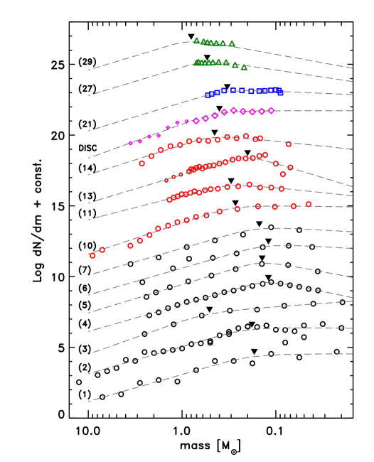
Figure 1.— Mass functions of selected clusters in our sample (see Table 1 for the ID numbers). The data for YCs are shown as large circles (except for Praesepe, where also small circles are used to show the MF at the high-mass end as measured by Williams et al. (1995); NGC 6397 is shown as representative for the class of dense GCs (squares); while the MFs of loose GCs are indicated by triangles (only NGC 2298 and NGC 6712 are shown). The typical $1\,\sigma$ uncertainty on the MF is $0.5$ dex at $\sim 0.3$ M_⊙ . The dashed lines represent the best fitting TPL distributions, as per the parameters of Table 1, with the values of $m_{c}$ indicated by the dark down-pointing triangles. For reference, we also show the MF of the Galactic disc. At the low-mass end the data are those recently obtained by Covey et al. (2008) from Sloan Digital Sky Survey and Two Micron All Sky Survey data (large diamonds), whereas above $\sim 1$ M_⊙ we show the MF obtained by Reid et al. (2002) and corrected for the effects of stellar evolution (small diamonds).

3. The data sample

The data used in this work come from a number of different sources. As regards GCs, we considered the entire HST sample of Paresce & De Marchi (2000), which is made up of twelve relatively dense clusters, and added to it four low-concentration GCs studied by our team in recent years (for details see Table 1). De Marchi et al. (2007) showed that a strong trend exists between a cluster’s central concentration $c$ (defined as the logarithmic ratio of the tidal radius and core radius) and the shape of its present stellar MF: dense GCs, i.e. those with $c>1.5$, have a relatively steep MF with an average power-law index of $-1.5$ in the range $0.3-0.8$ M_⊙ , while loose GCs with $c<1.5$ show a much flatter or even inverted MF over the same mass range. Several interpretations exist for this result (e.g. Baumgardt, De Marchi & Kroupa 2008; Kruijssen & Portegies Zwart 2009; Vesperini, McMillan & Portegies Zwart 2009; Kruijssen 2009), but they all point to a shorter time to dissolution for loose GCs. For this reason, it is important to cover both dense ($c>1.5$) and loose ($c<1.5$) clusters when studying the temporal evolution of the stellar MF.

As regards YCs, the data cover high quality observations of fourteen star-forming regions and associations of various ages, as shown in Table 1. For each YC, we searched for the most accurate determination of the MF in the recent literature (see references in Table 1), looking specifically for information on the number of stars measured in each mass bin. In those cases in which the MFs were not directly available in tabular form, we extracted the data points (i.e. number of stars in each mass bin) from the published graphs, but we specifically ignored any fits (with power-law or log-normal functions) or interpolations of these data that the various authors may have carried out. The MFs in our sample were determined either by converting an observed luminosity function via a theoretical mass–luminosity relationship or by counting the number of stars falling between evolutionary tracks in a color–magnitude or Hertzsprung–Russell diagram. We only restricted our search to works in which the MF is based on known cluster members and a correction for photometric incompleteness has been applied to the luminosity function, if needed. Furthermore, to guarantee that the sample is as homogeneous as possible, we have ignored any corrections to the MF meant to account for the presence of binaries, since these are rather uncertain and only available in a limited number of cases. Therefore, the MFs that we consider in this study, for both YCs and GCs, are the MFs of stellar systems, i.e. we do not distinguish between single and multiple stars.

In order to prevent biases in the results, the data should refer to the global MF (GMF), i.e. to the MF of the cluster as a whole. For GCs, where complete cluster coverage is not always possible, we used information on mass stratification and mass segregation to derive the GMF from the local MF (see e.g. De Marchi et al. 2006). Alternatively, we used the MF measured near the half-light radius (i.e. the effective radius containing half of the cluster’s luminosity, see e.g. Portegies Zwart, McMillan & Gieles 2010), since it has been shown to reflect quite reliably the properties of the GMF (De Marchi et al. 2000). For YCs, we specifically selected those objects and studies for which the coverage is as complete as possible.

We then performed a multivariate fit to each MF with a TPL distribution and derived the values of the parameters $\alpha$, $\beta$ and $m_{c}$ that simultaneously provide the smallest residuals. The values of the best fitting parameters and their associated $1\,\sigma$ uncertainties are given in Table 1 for all the clusters in our sample. The MFs of a few selected clusters are also shown graphically in Figure 1, together with the best TPL fits as per the parameters of Table 1. We compare and discuss the results of our best fits in Section 5, but we precede that with a short discussion on the value of $\alpha$.

4. Mass function shape above $\sim 0.8$ M_⊙ 

In the TPL distribution described by Equation 1, the value of $\alpha$ determines the shape of the MF above the characteristic mass $m_{c}$. Since the data for GCs do not constrain the mass range above the main-sequence turn-off ($>0.8$ M_⊙), we had to assume a value of $\alpha$ for those objects. An obvious first choice would be the slope of the Salpeter (1955) IMF, namely $\alpha=-2.35$. According to Kroupa (2002), that is the average value of the slope of the stellar MF in clusters and associations above $0.5$ M_⊙ . However, this is not a meaningful average because of the very large scatter at $m>1$ M_⊙ displayed by the MF slopes included in Kroupa’s (2002) compilation, which in turn are taken from Scalo (1998). In fact, after discussing with this latter author (J. Scalo, priv. comm.), we realised that the $\alpha=-2.35$ value obtained in that way is not a meaningful average. It is also not consistent with any of the individual $\alpha$ values that we measure for the YCs in Table 1, except for Taurus and possibly Pleiades.

As an alternative we could use the MF of the Galactic disc, but decided against it because of the large uncertainties involved. The most recent determination is that by Covey et al. (2008) using Sloan Digital Sky Survey and 2 MASS data, although these observations do not reach above $\sim 1$ M_⊙ (see large diamonds in Figure 1). To extend the MF to higher masses, these authors use the measurements of Reid, Gizis & Hawley (2002). We do the same and show with small diamonds in Figure 1 the MF that Reid et al. (2002) obtained using an empirical mass–magnitude relationship and after correction for the effects of stellar evolution (this provides them with an estimate of the IMF). The best fit with a TPL distribution gives $\alpha=-2.4\pm 0.4$, $\beta=2.3\pm 0.4$ and $m_{c}=0.4\pm 0.05$, revealing again a rather large uncertainty around the value of $\alpha$.

In the end, following the suggestion of an anonymous referee, we concluded that the most appropriate value of $\alpha$ to adopt for GCs is the average of the best fitting $\alpha$ values that we obtain in the same mass range for YCs, namely $\alpha=-1.97\pm 0.17$. This is also conveniently very close to the value that Van Buren (1985) found for the MF slope in the range $5-120$ M_⊙ from a detailed analysis of the all-sky sample of O stars of Garmany, Conti & Chiosi (1982) that makes use of high-resolution extinction maps derived spectroscopically to account for the effects of obscuration on star counts (Scalo 1986).

Finally, we note that observational constraints on the initial value of $\alpha$ for GCs could in principle come from the analysis of the white dwarf luminosity function. The results of Richer et al. (2004) on the white dwarf cooling sequence of M 4 (NGC 6121) seem to suggest a value in the range $-2.5<\alpha<-1.5$, but more recent work by the same team (Richer et al. 2008) on another cluster, NGC 6397, seems to require a much steeper slope, possibly as large as $\alpha\simeq-5$. Therefore, it appears that the uncertainties are presently still too large for this method to place meaningful empirical constraints on the value of $\alpha$ for GCs, although progress in this field is likely with the advent of the James Webb Space Telescope in the near future.

5. Evolution of the mass function

The mean $\alpha$ and $\beta$ values for the YCs in our sample, resulting from our best fits shown in Table 1, are respectively $-1.97\pm 0.17$ and $2.51\pm 0.62$ ($1\,\sigma$ standard deviation uncertainties). For GCs, having assumed $\alpha\equiv-2$, we find $\beta=2.49\pm 0.47$. In spite of the widely different physical properties of the clusters in our sample, e.g. in terms of chemical composition, total mass, stellar density and age (see Table 1), the values of $\alpha$ and $\beta$ span a relatively narrow range and, in particular, there is no significant difference in $\beta$ between YCs and GCs. Obviously, having assumed $\alpha\equiv-2$ for GCs has in principle a systematic effect on $\beta$, but this does not seem to be large (an even smaller effect on $m_{c}$ is discussed below). For example, with our original assumption of $\alpha\equiv-2.35$ we found $\beta=2.6\pm 0.3$. This suggests that that there does not seem to be substantial difference in the way the stellar MF rises to and falls from its peak, i.e. the characteristic mass, in clusters covering a wide range of physical properties, including age, chemical composition, total mass and density.

Where large differences are seen, however, is in the value of the characteristic mass itself. The average value of $m_{c}$ for dense GCs is $0.31\pm 0.03$ M_⊙ and for loose globulars it grows to $0.64\pm 0.10$ M_⊙, although the statistics here is limited. As noted above, the actual value of $m_{c}$ depends in principle on the assumed $\alpha$, but changing the latter by $0.4$ would cause $m_{c}$ to vary by just $0.01$ M_⊙ for the GCs in our sample. It is therefore unlikely that the differences in the $m_{c}$ values that we observe are just the result of uncertainties in $\alpha$. The variation in $m_{c}$ is equally large for YCs, ranging from $0.12$ M_⊙ to $0.51$ M_⊙, and here the data provide much more solid constraints on the value of $\alpha$.

In principle, all these $m_{c}$ variations could reflect differences in the star formation process, in turn resulting from differences in the physical conditions of the environment (e.g. Larson 2005 and references therein). However, as the data in Table 1 show, there does not seem to be any correlation between the value of $m_{c}$ and the clusters’ physical properties such as total mass, concentration, age or metallicity.

For example, the dense GCs in our sample span almost two decades in metallicity and total mass, but have practically the same $m_{c}$, while all YCs have practically the same metallicity but a wide range of $m_{c}$ values. Therefore, if the environment plays a role in determining the shape of the stellar MF this effect does not seem to be the dominant one, at least not for the clusters in our sample. In fact, taken at face value, the data in Table 1 show no sign of such an effect.

A more interesting possibility to consider in order to explain the observed spread in $m_{c}$ is the role of dynamical evolution, which could alter the shape of the MF over time because of the preferential loss of low-mass stars caused by the two-body relaxation process. It is thus worth investigating whether our data show any correlation or trend between the characteristic mass and the dynamical state of the cluster.

For this reason we have listed in Table 1 the dynamical age $\tau_{\rm dyn}$ of each cluster, expressed as $t/t_{\rm dis}$ or the cluster age $t$ in units of the dissolution time $t_{\rm dis}$, in turn defined as the time at which the cluster has lost 95 % of its original mass. Using N-body models, Baumgardt & Makino (2003; hereafter BM03) showed that $t_{\rm dis}\propto t^{x}_{\rm rh}t^{1-x}_{\rm cr}$ where $t_{\rm rh}$ is the half-mass relaxation time, $t_{\rm cr}$ the crossing time and $x$ depends on the initial concentration of the cluster $W_{0}$. Later, Gieles et al. (2005), using the same N-body models, found that $t_{\rm dis}$ can also be expressed as a function of the total initial mass of the cluster $M_{\rm ini}$ as $t_{\rm dis}\propto t_{0}M_{\rm ini}^{0.62}$ (see also Gieles 2010), where the tidal disruption parameter $t_{0}$ depends on the properties of the host galaxy and on the cluster’s orbit.

The values of $\tau_{\rm dyn}$ listed in Table 1 come from Baumgardt et al. (2008) for the specific GCs in our sample and take into account the differences that exist between their orbital parameters. As regards the YCs in the sample, they are all located in the solar neighbourhood and should therefore experience rather similar interactions with the Galaxy. This is consistent with the results of Lamers et al.’s (2005) study of the age distribution of open clusters in the solar neighbourhood within 600 pc, based on the catalogue by Kharchenko et al. (2005). They conclude that $t_{0}=3.3^{+1.5}_{-1.0}$ Myr, so if we accept an uncertainty of $\sim$$1/3$ on the value of $t_{\rm dis}$, we can ignore its dependence on the specific cluster’s orbit. The individual $t_{\rm dis}$ values for the YCs in our sample can then be derived following BM03’s N-body simulations for clusters with low initial concentration $W_{0}=5$ and a distance of $R_{G}=8.5$ kpc from the Galactic centre.

Using BM03’s Figure 1a, we have estimated the initial mass $M_{\rm ini}$ of our clusters from their present-day total mass $M_{\rm tot}$ and age $t$ as given in Table 1. While BM03 consider clusters with an initial number of stars $N$ ranging from 8K to 128K objects, for ages younger than $\sim 650$ Myr, as is the case for all YCs in our sample, the ratio $M_{\rm tot}/M_{\rm ini}$ varies only marginally with $N$, at most by 10 % and only imperceptibly for $t<300$ Myr. We have therefore followed the curve for $N=$32K in Figure 1a of BM03 to derive the estimated value of $M_{\rm ini}$, which we have then used to derive the time to dissolution $t_{\rm dis}$ and hence $\tau_{\rm dyn}$ by means of Figure 3 in that same paper, again following the distribution for clusters with $R_{G}=8.5$ kpc and $W_{0}=5$. For clusters younger than 100 Myr we have assumed $t_{\rm dis}\simeq 500$ Myr but our conclusions would not change if $t_{\rm dis}$ were larger or smaller by a factor of two for these clusters.

It is to be expected that the values of $\tau_{\rm dyn}$ derived in this way are somewhat uncertain, even though they are as accurate as one can obtain based on the available information. Lamers et al. (2005) point out that the disruption times obtained by BM03 are most likely an upper limit because they are calculated for tidal disruption in a smooth tidal field without other destruction mechanisms. Hereafter we will assume an uncertainty of about $45\,\%$ on $t_{\rm dis}$, which combined with a typical accuracy of $\sim 20\,\%$ on cluster ages implies an uncertainty of about $50\,\%$ on $\tau_{\rm dyn}$.

The relatively high $\tau_{\rm dyn}$ value of the Hyades is consistent with the conclusion of Perryman et al. (1998) that this cluster has lost about $3/4$ of its original mass. Conversely, Praesepe might not be as dynamically old as the estimated value of $\tau_{\rm dyn}$ would suggest if it is confirmed that the cluster is indeed the result of a merger of two clusters with different ages (see Holland et al. 2000; Franciosini, Randich & Pallavicini 2003). Finally, a particularly interesting case is that of Taurus. Ballesteros–Paredes et al. (2009) conducted a gravitational analysis of its orbit and concluded that the Taurus molecular cloud must be suffering significant tidal disruption, in spite of its young age (1 Myr). We conservatively assigned to it $\tau_{\rm dyn}=$ $1/2$, although the actual value could be larger.

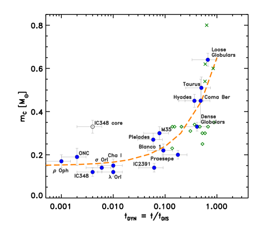
Figure 2.— Run of the characteristic mass $m_{c}$ as a function of the dynamical age $\tau_{\rm dyn}$. Dense and loose GCs are indicated, respectively, with diamonds and crosses, with a filled circle providing the average value of each class. The core of IC 348 is indicated as an open circle to distinguish it from the whole cluster. The dashed line is an eye-ball fit to the data.

The run of $m_{c}$ as a function of $\tau_{\rm dyn}$ is shown in Figure 2, where all clusters are labeled individually, except for the GCs (see caption for details). The figure reveals a rather remarkable trend of increasing $m_{c}$ with dynamical age over the entire range covered by the data. The dashed line is a purely empirical eye-ball fit to the data with the relationship

$$m_{c}/M_{\odot}\simeq 0.15+0.5\times\tau_{\rm dyn}^{3/4}$$ (2)

although an index of $1/2$ would still give an acceptable fit. Equally remarkable in Figure 2 is the absence of dynamically young clusters with large $m_{c}$ but even more striking, considering the logarithmic scale of the abscissa, is the lack of dynamically old objects ($\tau_{\rm dyn}>0.3$) with a small $m_{c}$, even for GCs with a total mass of order $10^{6}$ M_⊙ .

There are several effects that can cause the scatter seen in Figure 2 around the dashed line, including the uncertainty on $\tau_{\rm dyn}$ and $m_{c}$, the role of binaries and incomplete coverage of the clusters. As an example of the latter, we show in Figure 2 also the data point corresponding to the sole central regions of IC 348 (from the MF of Muench et al. 2003). In spite of the young age of the cluster, the MF in its core shows strong signs of mass segregation, with $m_{c}=0.33$ M_⊙ as opposed to $m_{c}=0.12$ M_⊙ for the cluster as a whole. This may be due to primordial mass segregation and/or to very fast dynamical evolution (see e.g. Allison et al. 2009), but in either case this data point should be excluded from the sample in order to not skew the results. In spite of our attempts to select only clusters with complete radial coverage, however, this information might not be completely available or fully correct in the literature. This is likely to cause a larger uncertainty on $m_{c}$ than what we obtain through the TPL fit to the MF and could account for some of the residual scatter that we observe. An additional source of uncertainty on $m_{c}$ comes from the fact that all the MFs considered here are system MFs, i.e. we do not attempt to correct for the presence of binaries. For dense GCs the binary fraction is just a few percent (Davis et al. 2008) and is not expected to significantly alter the value of $m_{c}$, but it is very likely higher for loose GCs and YCs (Sollima et al. 2007; 2010) and its effect should be considered. We will do so in a forthcoming paper. Finally, as mentioned above the uncertainty on the value of $\tau_{\rm dyn}$ can be important and this is witnessed by the size of the error bars that we show in Figure 2.

6. Discussion and conclusions

At least qualitatively, the trend seen in Figure 2 is fully consistent with the onset of mass segregation via two-body relaxation in a tidal environment, causing the preferential loss of low-mass stars from the cluster and hence a drift of the characteristic mass towards higher values. Vesperini & Heggie (1997) showed from N-body models that stellar evaporation, integrated over the cluster’s orbit and further enhanced by the presence of the Galactic tidal field, causes a flattening of the MF, i.e. a selective depletion at the low-mass end. Their models do not reveal a drift of the characteristic mass towards higher values, but their IMF in all cases is a pure power-law. A drift of $m_{c}$ is visible in the N-body models of Portegies Zwart et al. (2001), although it proceeds very slowly and only appears when the study of the MF is limited to the regions inside the half-mass radius.

That mass segregation is present in both young and globular clusters has long been established observationally. Examples include many of the YCs in our sample, such as M 35 (e.g. Mathieu 1983; Barrado y Navascués et al. 2001), Pleiades (e.g. Converse & Stahler 2008), Hyades (Reid 1993; Perryman et al. 1998), Blanco 1 (Moreaux et al. 2007). As for GCs, mass segregation has been observed in all those objects where MF measurements exist at various radial distances (see e.g. De Marchi et al. 2007 and references therein) and can be satisfactorily explained as being the result of the two-body relaxation process (Spitzer 1987). Furthermore, De Marchi et al. (2007) have also shown that dense and loose GCs have today systematically different GMFs and this is consistent with a much stronger selective loss of low-mass stars in the latter. Loose GCs have systematically larger $m_{c}$ than denser clusters with otherwise similar metallicity or space motion parameters. This strongly suggests that the value of $m_{c}$ must drift as a result of the cluster’s dynamical evolution, which is quicker in loose systems, even though the analysis of the N-body models (e.g. Portegies Zwart et al. 2001) has so far failed to detect this effect. In fact, Kruijssen (2009) has recently developed a simple physical model for the evolution of the MF that builds on the pioneering work of Hénon (1969). His results (see Figure 14 in Kruijssen 2009) show a shift in the inflection point of the MF with evolutionary time, consistent with a drift in $m_{c}$ (D. Kruijssen, priv. comm.).

A potentially very interesting consequence of the trend shown in Figure 2, if dynamical evolution is indeed at its origin, is that it would seem plausible that all GCs, having now $m_{c}\simeq 0.33$ M_⊙ if they are dense or $\sim 0.65$ M_⊙ if they are loose, were born with a stellar MF like the one measured today in the youngest Galactic clusters, or more precisely with $m_{c}\simeq 0.15$ M_⊙. Although not necessarily required by Figure 2, this scenario is consistent with it.

The careful reader will notice that this statement appears at odds with the conclusions of a previous work by our team. From a study of the GMFs of twelve halo GCs with widely different dynamical histories and noting that they show a very similar characteristic mass ($m_{c}=0.33\pm 0.03$ M_⊙ ), Paresce & De Marchi (2000) concluded that this value of $m_{c}$ had to be a feature of the stellar IMF in GCs. However, it is now apparent that this conclusion was the result of a selection effect, due to the fact that all twelve GCs in the Paresce & De Marchi (2000) sample have high central concentration, since no reliable information on the low-mass end of the MF of loose GCs was available at that time. The analysis presented by De Marchi et al. (2007) suggests that dense GCs have lost less low-mass stars than looser clusters throughout their life, but this does not mean that they have lost none. Therefore, one can no longer conclude that the $m_{c}\simeq 0.33$ M_⊙ value observed in the present-day GMF of dense GCs reflects the characteristic mass of their IMF, since it could have been smaller.

The possibility that GCs were born with a much smaller $m_{c}$ value than what we measure today in their MF would also be consistent with the absence of a turn-over in the MF of the Galactic bulge down to the observational limit at $\sim 0.2$ M_⊙ (Zoccali et al. 2000). Regardless as to whether the bulge is primarily the result of fast formation at early epochs (e.g. Ballero et al. 2007) or a collection of the stars lost from disrupted clusters throughout the life of the Galaxy (e.g. Gnedin & Ostriker 1997), its very location at the bottom of the Galaxy’s potential well makes it very hard for low-mass stars to escape from it. Therefore, while the present MF of the Galactic disc could represent a complex average over time and space, that of the bulge should have not been altered by dynamical evolution and, unlike the case of the comparably old GCs, should still reflect the properties of the IMF. Forthcoming HST observations of the Galactic bulge (see e.g. Brown et al. 2009) will provide insights on its MF below $0.15$ M_⊙, where we expect a turn-over.

To be sure, N-body models of dense stellar systems able to deal with a large number of particles ($N>10^{6}$) and incorporating a realistic treatment of stellar evolution and of the interaction with the Galactic tidal field (see Portegies Zwart et al. 2010) would be necessary to simulate the growth of the characteristic mass with time in GCs. Our analysis (see Section 5) suggests that young and globular clusters may share rather similar values of the $\alpha$ and $\beta$ parameters. Thus, if the picture sketched above is correct and, by strongly affecting the value of $m_{c}$, dynamical evolution act as the main source of variations in the present-day stellar MF of Galactic clusters, one might postulate that Population I and II stars should have similar IMFs. While not necessarily required by our analysis, this hypothesis is fully compatible with our results. Claims of the IMF universality that one finds in the literature (e.g. Gilmore 2001; Elmegreen et al. 2008) are based on the observation that stellar MFs in different environments have similar $m_{c}$ values, within a factor of a few. Here we show that it is plausible that the original value of $m_{c}$ be actually the same for Population I and II stars.

If this is true, one would have to consider the possibility that the characteristic mass in the IMF is not necessarily set by the Jeans mass scale in the forming cloud (e.g. Larson 1998; Larson 2005) and that the physical conditions of the environment do not play a significant role in the outcome of the star formation process, i.e. on the IMF. This, however, would not necessarily mean that the star formation process itself is the same: recent numerical simulations proposed by Goodwin & Kouwenhoven (2009) and Bate (2009) suggest that the IMF shape is largely insensitive to parameters such as the binary fraction and mass ratio in binaries. If this is the case, the role of the IMF as an effective tool to probe the physics of star formation may have to be critically reconsidered.

References

- Allison et al. (2009) Allison, R., Goodwin, S., Parker, R., de Grijs, R., Portegies Zwart, S., Kouwenhoven, M. 2009, ApJ, 700, L99
- Ballesteros–Paredes et al. (2009) Ballesteros–Paredes, J., Gomez, G., Loinard, L., Torres, R., Pichardo, B. 2009, MNRAS, 395, L81
- Ballero et al. (2007) Ballero, S., Matteucci, F., Origlia, L., Rich, M. 2007, A&A, 467, 123
- Barrado y Navascues et al. (2001) Barrado y Navascués, D., Stauffer, J., Bouvier, J., Martin, E. 2001, ApJ, 546, 1006
- Barrado y Navascues et al. (2004a) Barrado y Navascués, D., Stauffer, J., Bouvier, J., Jayawardhana, R., Cuillandre, J.-C. 2004, ApJ, 610, 1064
- Barrado y Navascues et al. (2004b) Barrado y Navascués, D., Stauffer, J., Jayawardhana, R. 2004, ApJ, 614, 386
- Bate (2009) Bate, M. 2009, MNRAS, 397, 232
- Baumgardt, De Marchi & Kroupa (2008) Baumgardt, H., De Marchi. G., Kroupa, P. 2008, ApJ, 685, 247
- Baumgardt & Makino (2003) Baumgardt, H., Makino, J. 2003, MNRAS, 340, 227
- Bouvier et al. (2008) Bouvier, J. et al. 2008, A&A, 481, 661
- Brown et al. (2009) Brown, T. et al. 2009, AJ, 137, 317
- Caballero (2008) Caballero, J. 2008, A&A, 478, 667
- Chabrier (2003) Chabrier, G. 2003, PASP, 115, 763
- Chappelle et al. (2005) Chappelle, R., Pinfield, D., Steele, I., Dobbie, P., Magazzù, A. 2005, 361, 1323
- Converse & Stahler (2008) Converse, J., Stahler, S. 2008, ApJ, 678, 431
- Corey et al. (2008) Corey, K. et al. 2008, AJ, 136, 1778
- Davis et al. (2008) Davis, D., Richer, H., Anderson, J., Brewer, J., Hurley, J., Kalirai, J., Rich, R., Stetson, P. 2008, AJ, 135, 2155
- De Marchi, Paresce & Portegies Zwart (2005) De Marchi, G., Paresce, F., Portegies Zwart, S. 2005, in The Initial Mass Function 50 years later, eds. E. Corbelli, F. Palla, H. Zinnecker (Dordrecht: Springer), 77
- De Marchi, Paresce & Pulone (2000) De Marchi, G., Paresce, F., Pulone, L. 2000, ApJ, 530, 342
- De Marchi, Paresce & Pulone (2007) De Marchi, G., Paresce, F., Pulone, L. 2007, ApJ, 656, L65
- De Marchi, Pulone & Paresce (2006) De Marchi, G., Pulone, L., Paresce, F. 2006, A&A, 449, 161
- Dolan & Mathieu (2002) Dolan, C., Mathieu, R. 2002, AJ, 123, 387
- Elmegreen (2010) Elmegreen, B. 2010, in IAU Symp. 266, eds. R. de Grijs, J. Lepine (Cambridge: CUP), 3
- Elmegreen, Klessen & Wilson (2008) Elmegreen, B., Klessen, R., Wilson, C. 2008, ApJ, 681, 365
- Forbes & Bridges (2010) Forbes, D., Bridges, T. 2010, MNRAS, 404, 1203
- Franciosini, Randich & Pallavicini (2003) Franciosini, E., Randich, S., Pallavicini, R. 2003, A&A, 405, 551
- Garmany, Conty & Chiosi (1982) Garmany, D., Conti, P., Chiosi, C. 1982, ApJ, 263, 777
- Gieles et al. (2005) Gieles, M., Bastian, N., Lamers, H., Mout, J. 2005, A&A, 441, 949
- Gieles (2010) Gieles, M. 2010, in IAU Symp. 266, eds. R. de Grijs, J. Lepine (Cambridge: CUP), 69
- Gilmore (2001) Gilmore, G. 2001, in Starburst Galaxies, eds. L. Tacconi, D. Lutz (Heidelberg: Springer), 34
- Gnedin & Ostriker (1997) Gnedin, O., Ostriker, J. 1997, ApJ, 474, 223
- Goodwin & Kouwenhoven (2009) Goodwin, S., Kouwenhoven, M. 2009, MNRAS, 397, L36
- Harris (1996) Harris, W. 1996, AJ, 112, 1487
- Hodapp et al. (2009) Hodapp, K., Iserlohe, C., Stecklum, B., Krabbe, A. 2009, ApJ, 701, L100
- Holland et al. (2000) Holland, K., Jameson, R., Hodgkin, S., Davies, M., Pinfield, D. 2000, MNRAS, 319, 956
- Kharchenko et al. (2005) Kharchenko, N. Pisnukov, A. E., Röser, S., Schilbach, E., Scholz, R. 2005, A&A, 438, 1163
- Kraus & Hillenbrand (2007) Kraus, A., Hillenbrand, L. 2007, AJ, 134, 2340
- Kroupa (2002) Kroupa, P. 2002, in Modes of Star Formation and the Origin of Field Populations, ASP Conf. Ser. 285, eds. E. Grebel, W. Brandner (San Francisco: ASP), 86
- Kruijssen (2009) Kruijssen, D. 2009, A&A, 507, 1409
- Kruijssen & Portegies Zwart (2009) Kruijssen, J., Portegies Zwart, S. 2009, ApJ, 698, L158
- Kücük & Akkaya (2010) Kücük, I., Akkaya, I. 2010, RMxAA, 46, 109
- Lada & Lada (2003) Lada, C., Lada, E. 2003, ARAA, 41, 57
- Lamers et al. (2005) Lamers, H., Gieles, M., Bastian, N., Baumgardt, H., Kharchenko, N., Portegies Zwart, S. 2005, A&A, 441, 117
- Larson (1998) Larson, R. 1998, MNRAS, 301, 569
- Larson (2005) Larson, R. 2005, MNRAS, 359, 211
- Luhman (2007) Luhman, K. 2007, ApJS, 173, 104
- Luhman & Rieke (1999) Luhman, K., Rieke, G. 1999, ApJ, 525, 440
- Mathieu (1983) Mathieu, R. 1983, ApJ, 267, L97
- Moraux et al. (2007) Moraux, E., Bouvier, J., Stauffer, J., Barrado y Navascués, D., Cuillandre, J.-C. 2007, A&A, 471, 499
- Moraux et al. (2003) Moraux, E., Bouvier, J., Stauffer, J., Cuillandre, J.-C., 2003, A&A, 400, 891
- Muench et al. (2003) Muench, A. et al. 2003, AJ, 125, 2029
- Paresce & De Marchi (2000) Paresce, F., De Marchi, G. 2000, ApJ, 534, 870
- Perryman et al. (1998) Perryman, M., et al. 1998, A&A, 331, 81
- Piskunov et al. (2008) Piskunov, A., Schilbach, E., Kharchenko, N. V., Röser, S., Scholz, R. 2008, A&A, 477, 165
- Portegies Zwart et al. (2010) Portegies Zwart, McMillan, S., Gieles, M. 2010, ARAA, in press (astro-ph/1002.1961)
- Portegies Zwart et al. (2001) Portegies Zwart, McMillan, S., Hut, P., Makino, J. 2001, MNRAS, 321, 199
- Reid (1993) Reid, N. 1993, MNRAS, 265, 785
- Reid, Gizis & Hawley (2002) Reid, N., Gizis, J., Hawley, S. 2002, AJ, 124, 2721
- Richer et al. (2004) Richer, H. et al. 2004, AJ, 127, 2771
- Richer et al. (2008) Richer, H. et al. 2008, AJ, 135, 2141
- Salas & Cruz–Gonzalez (2010) Salas, L., Cruz–Gonzalez, I. 2010, RMxAA, 46, 37
- Salpeter (1955) Salpeter, E. 1955, ApJ, 121, 161
- Scalo (1986) Scalo, J. 1986, Fund. Cos. Phys., 11, 1
- Slesnick et al. (2004) Slesnick, C. Hillenbrand, L., Carpenter, J. 2004, ApJ, 610, 1045
- Sollima et al. (2007) Sollima, A., Beccari, G., Ferraro, F., Fusi Pecci, F., Sarajedini, A. 2007, MNRAS, 380, 781
- Sollima et al. (2010) Sollima, A., Carballo–Bello, J., Beccari, G., Ferraro, F., Fusi Pecci, F., Lanzoni, B. 2010, MNRAS, 401, 577
- Spitzer (1987) Spitzer, L. 1987, Dynamical evolution of globular clusters, (Princeton: PUP)
- Van Buren (1985) Van Buren, D. 1985, ApJ, 294, 567
- Vesperini & Heggie (1997) Vesperini, E., Heggie, D. 1997, MNRAS, 289, 898
- Vesperini et al. (2009) Vesperini, E., McMillan, S., Portegies Zwart, S. 2009, ApJ, 698, 615
- William, Rieke & Stauffer (1995) Williams, D., Rieke, G., Stauffer, J. 1995, ApJ, 445, 359
- Zoccali et al. (1999) Zoccali, M., et al. 2000, ApJ, 530, 418