Logarithmic bred vectors in spatiotemporal chaos: structure and growth

Abstract

Bred vectors are a type of finite perturbation used in prediction studies of atmospheric models that exhibit spatially extended chaos. We study the structure, spatial correlations, and the growth-rates of logarithmic bred vectors (which are constructed by using a given norm). We find that, after a suitable transformation, logarithmic bred vectors are roughly piecewise copies of the leading Lyapunov vector. This fact allows us to deduce a scaling law for the bred vector growth rate as a function of their amplitude. In addition, we relate growth rates with the spectrum of Lyapunov exponents corresponding to the most expanding directions. We illustrate our results with simulations of the Lorenz ’96 model.

I Introduction

In dynamical systems theory, chaos is usually defined on the basis of the exponential departure of infinitesimally separated initial conditions. The exponential law stems from the linearity of the equations that govern infinitesimal perturbations. In applications, however, errors are typically finite. This occurs, for instance, in the breeding method used to generate finite perturbations for ensemble forecasting at the National Centers for environmental Prediction (USA) TothKalnay1993 ; kalnay . Bred vectors are closely related to Lyapunov vectors (LVs) albeit different since they are finite by construction and result from the evolution of perturbations, which are imposed to have a certain size via periodic normalizations. One advantage of bred vectors in applications is that the model under study does not have to be linearized, in contrast with LVs. (Keep in mind that the linearization of a meteorological model is a delicate question due to the presence of nondifferentiable or discrete programming structures, see e.g. tlm .) The drawback is that bred vectors are governed by fully nonlinear models, what constitutes a challenge for their theoretical description.

In this article we use a special class of bred vector, the so-called logarithmic bred vector (Log-BV) Primo2005 ; Primo2006 , which has the particularity of being normalized using the geometric (or zero) norm. This choice has proven to be the most convenient for spatially extended systems (see Ref. Primo2005 ; Primo2006 ) and offers some advantages in theoretical terms. We will focus on two aspects of bred vectors: First, we uncover common structural properties of Log-BVs and the leading LV. In the second part of the paper we study the growth rate of Log-BVs, which we shall refer to as bred exponents (BEs) —instead of the more imprecise term finite-size Lyapunov exponents Boffetta2002 — for the sake of brevity and to emphasize their origin. We find an interesting relation between BEs and Lyapunov exponents (LEs) of spatio-temporally chaotic systems.

This paper is organized as follows: In Sec. II we introduce the Lorenz ’96 model, which we will use throughout this contribution in order to illustrate our considerations. For the parameter values selected the Lorenz ’96 is hyperchaotic and exhibits spatio-temporal chaos. In the following section we explain the computation of Log-BVs. A surface picture is introduced for the leading LV in Sec. IV.1 and extended to analyze Log-BVs in Sec. IV.2. In Sec. V we study the growth rates (i.e., BEs) of Log-BVs. In Sec. V.1 the convergence to the largest LE is found to obey a scaling relation. In Sec. V.2 we explain how the BEs are related to the spectrum of LEs. The conclusions are summarized in Sec. VI.

II The Lorenz ’96 model

The Lorenz ’96 model Lorenz1996 ; Lorenz1998 is a toy model originally proposed in the context of atmospheric dynamics and used extensively to test novel techniques and applications. It is a time continuous model consisting of a set of nonlinear ODEs coupled in a ring geometry:

$$\frac{d\,u(x,t)}{dt} = -u(x,t)-u(x-1,t)u(x-2,t)$$ (1)

$$\quad+u(x-1,t)u(x+1,t)+F,\quad$$

$$\mbox{with}\quad x=1,...,L.$$

$u(x,t)$ can be seen as a scalar meteorological variable, e.g. temperature, at $L$ equally spaced sites $x$ on a latitude circle (and hence periodic boundary conditions are assumed). Moreover, there is an external forcing constant $F$ that mimics the solar driving of the atmosphere.

For $L>3$ the solutions of (1) are chaotic if $F$ is large enough. In particular the steady solution $u(x,t)=F$ becomes unstable if $F>8/9$ Lorenz1998 . A more detailed study shows that stable nonchaotic solutions survive up to a value of $F$ that, though depending on $L$, is approximately in the range 4 to 6 Lorenz2006 . Beyond some threshold value of $F$, chaotic dynamics of the model becomes fully developed. More precisely, the dynamics is extensive with $L$ (see e.g. results in Karimi2009 for $F=10$). Extensivity means that many relevant quantities (dimension, entropy, etc.) scale linearly with the system size, and the LEs $\{\lambda_{n}\}_{n=1,\ldots,L}$ converge to a density in the “thermodynamic” limit $L\to\infty$. This property is shared by a number of extended dynamical systems ranging from coupled map lattices to PDEs such as the Kuramoto-Sivahinsky or the complex Ginzburg-Landau equations CrossHohenberg .

In order to compute bred and Lyapunov vectors and their growth rates in the Lorenz ’96 model, we integrate Eq. (1) and its linearization (tangent space) by using a fourth order Runge-Kutta-solver with time step $\Delta t=0.01$. Before measuring the quantities we are interested in, we allow the system to breed Log-BVs for a transient time $t_{trans}>8(L^{1.5})$.

III Logarithmic Bred Vectors and Breeding

In 1993, Toth and Kalnay TothKalnay1993 created a special operational cycle designed to “breed” fast growing errors in meteorological models. It uses finite perturbations that are periodically normalized to become bred vectors after some breeding cycles.

In the following we describe the procedure to compute bred vectors in mathematical terms. A control (unperturbed) trajectory $\mathbf{u}(t)=[u(x,t)]_{x=1}^{x=L}$ and a perturbed one $\tilde{\mathbf{u}}(t)=[\tilde{u}(x,t)]_{x=1}^{x=L}$ are evolved in parallel obeying Eq. (1). The difference between the perturbed and unperturbed trajectories is calculated every time interval $\tau$, say at times $\tau_{m}=m\tau$, with $m=1,2,\ldots$ to obtain

$$\delta{\mathbf{u}}(\tau_{m})=\tilde{\mathbf{u}}(\tau_{m})-\mathbf{u}(\tau_{m}).$$ (2)

These differences are then scaled down at $t=\tau_{m}$ to a given perturbation amplitude $\varepsilon_{0}$ by defining

$$\delta\mathbf{u}_{\varepsilon_{0}}(\tau_{m})=\varepsilon_{0}\frac{\delta\mathbf{u}(\tau_{m})}{\|\delta\mathbf{u}(\tau_{m})\|},$$ (3)

where $\delta\mathbf{u}_{\varepsilon_{0}}(x,\tau_{m})$ denotes the bred vector at time $\tau_{m}$, and is $\|\cdot\|$ a particular norm. The perturbed trajectory is then redefined by means of the bred vector:

$$\tilde{\mathbf{u}}(\tau_{m}^{+})=\mathbf{u}(\tau_{m})+\delta\mathbf{u}_{\varepsilon_{0}}(\tau_{m}),$$ (4)

with $\tau_{m}^{+}=\lim_{\nu\rightarrow 0}\tau_{m}+\nu$ referring to the same time $\tau_{m}$, but after the rescaling. Perturbed and unperturbed trajectories are again integrated forward in parallel until next rescaling scheduled at time $\tau_{m+1}$.

The definition of the bred vector contains two ingredients. One is the parameter $\varepsilon_{0}$ controlling the amplitude. The second ingredient is the norm to be used since different norms will produce different bred vectors. In recent works Primo2005 ; Primo2006 it was found that the $0$-norm (or geometric norm)

$$\|\delta\mathbf{u}(t)\|\equiv\lim_{q\to 0}\left[\sum_{x=1}^{L}|\delta u(x,t)|^{q}\right]^{1/q}=\prod_{x=1}^{L}|\delta u(x,t)|^{1/L},$$ (5)

is a convenient choice for breeding. Due to the multiplicative character of the linear dynamics the $0$-norm ought to produce bred vectors that, at different times, $\tau_{m}$ are the most statistically equivalent among them. The bred vectors constructed in this way are called logarithmic bred vectors (log-BVs) Primo2005 ; Primo2006 ; Pazo2010 .

IV Structure of logarithmic bred vectors

IV.1 The main Lyapunov vector

Before starting our analysis of the Log-BVs it is useful to recall recent results concerning the structure of the main (or leading) LV. In a dynamical system an infinitesimal perturbation evolves generically towards the leading Lyapunov vector $\mathbf{g}(t)$, which indicates the direction of maximal growth for perturbations integrated since the remote past. The orientation of the LV in tangent space depends on the position in the chaotic attractor (that can be parametrized by time). For extended chaotic systems, it is observed that the LV projects very inhomogeneously on space. More precisely, the vector localizes at some quite narrow region of the system GiacomelliPoliti1991 . But noticeably, this localization is dynamic and the localization center changes as time evolves, thus recovering the homogeneity of the system in a statistical sense. In the 90s Pikovsky and coworkers Pikovsky1994 ; PikovskyPoliti1998 found very useful for the theoretical analysis to associate a “surface” with the leading LV by means of a Hopf-Cole transformation, which in $d=1$ dimension reads:

$$h_{LV}(x,t)=\ln|g(x,t)|,$$ (6)

with ${\mathbf{g}}(t)=[g(x,t)]_{x=1}^{x=L}$. For a large family of systems PikovskyPoliti1998 , including the Lorenz ’96 model Pazo2008 , $h_{LV}(x,t)$ exhibits correlations in space and time which are described by the canonical Kardar-Parisi-Zhang (KPZ) equation of stochastic surface growth Kardar1986 . This mapping leads to interesting scaling properties for $h_{LV}(x,t)$. The average width $w=\langle(h_{LV}-\langle h_{LV}\rangle)^{2}\rangle^{1/2}$ scales with the length of the system Barabasi1995 ; Halpin-Healy1995 as $w\propto L^{\alpha}$; with $\alpha=1/2$ as in the KPZ equation in one dimension. This means that, at sufficiently long scales, $h_{LV}(x,t)$ appears as the path of a random walk in $d=1$. This self-affine profile translates into a power-law dependence of the structure factor (a spatial power spectrum) at small wavenumbers:

$$S(k)\propto k^{-(2\alpha+d)}\;\;{\rm for}\;\;k<\bar{k},$$ (7)

where $S(k)=\langle\hat{h}(k,t)\hat{h}(-k,t)\rangle_{t}$, and $\hat{h}(k,t)=\sum_{x}\exp(ikx)h(x,t)$. At short length scales, $k>\bar{k}$, non-universal short-range correlations are expected to appear due to the deterministic character of the system. However, below $\bar{k}$ universal scaling properties emerge and this is reflected in a spatial correlation that generically decays as $\sim k^{-2}$ in one dimension.

Figure 1: (color online) Upper panel: Surfaces associated with the LV and with the Log-BV with the smallest value of $\varepsilon_{0}$ used $\varepsilon_{0}^{min}=e^{-20}$ (Lorenz ’96 model with $F=8.0$ and $L=1024$). Lower panel: Snapshot of the difference fields $\eta_{\varepsilon_{0}}=h_{\varepsilon_{0}}(x,t)-h_{LV}(x,t)$ (curves are arbitrarily shifted to improve their visibility).

IV.2 The logarithmic bred vectors

Analogously to the surface associated with the leading LV in Eq. (6), one can define a surface

$$h_{\varepsilon_{0}}(x,t)=\ln|\delta u_{\varepsilon_{0}}(x,t)|$$ (8)

by Hopf-Cole transforming the Log-BV of amplitude $\varepsilon_{0}$.

The main LV evolves following linear equations and, therefore, only its direction in tangent space matters. However for a bred vector the norm plays a very important role through the periodic rescaling of the perturbations defined above. If the geometric norm is chosen, the spatial mean of the associated Log-BV surface is fixed to a given size $\varepsilon_{0}$:

$$\overline{h}=\frac{1}{L}\sum_{x=1}^{L}h_{\varepsilon_{0}}(x,t=\tau_{m})=\ln\varepsilon_{0}.$$ (9)

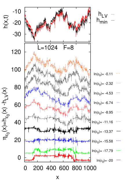
In the limit of small amplitude $\varepsilon_{0}\to 0$, the Log-BV aligns with the leading Lyapunov vector, and their profiles coincide, $h_{\varepsilon_{0}\to 0}(x,t)=h_{LV}(x,t)$, apart from an arbitrary constant due to the arbitrary norm (i.e. arbitrary $\bar{h}$) of the leading LV. This fact suggests that the leading LV can be a good reference point to analyze the structure of Log-BVs. In Fig. 1 we show a snapshot of the difference fields

$$\eta_{\varepsilon_{0}}(x,t)=h_{\varepsilon_{0}}(x,t)-h_{LV}(x,t).$$ (10)

We can see that, unless $\varepsilon_{0}$ is too large, $\eta_{\varepsilon_{0}}$ is mainly composed of plateaus, which indicates that the structure of $h_{\varepsilon_{0}}(x,t)$ is roughly a piecewise copy of $h_{LV}(x,t)$. Remarkably, this structure has been previously observed for LV-surfaces associated with LEs $\lambda_{n}$ ($n\geq 2$) smaller than the largest one $\lambda=\lambda_{1}$ Szendro2007 ; Pazo2008 . For the Log-BVs the typical plateau size decreases as $\varepsilon_{0}$ is increased, whereas for the sub-dominant LVs the plateau size is known Szendro2007 ; Pazo2008 to decrease as the index $n$ is increased ($\lambda_{n}\geq\lambda_{n+1}$). This suggests an interesting relation between both (Lyapunov and bred) vector types that is exploited below in Sec. V.2.

Note also that Primo et al. Primo2006 used the surface (8) to uncover several spatio-temporal scaling relations that already revealed in an indirect way the existence of cut-off lengths. These cut-off lengths are now apparent in the light of the plateaus in Fig. 1.

V bred exponents

We now focus on the (exponential) growth rate of Log-BVs, which we will refer to as bred exponents (BEs). We define the BEs as:

$$\lambda_{\varepsilon_{0}}=\frac{1}{\tau}\Big{\langle}\ln\frac{\|{\mathbf{\delta}\mathbf{u}}(\tau_{m}+\tau)\|}{\|{\mathbf{\delta}\mathbf{u}}_{\varepsilon_{0}}(\tau_{m})\|}\Big{\rangle},$$ (11)

with $\tau$ denoting the time between rescalings. $\lambda_{\varepsilon_{0}}$ can be seen as a type of finite-size Lyapunov exponent, see Appendix A of Boffetta2002 . The value of $\lambda_{\varepsilon_{0}}$ is not very sensitive to $\tau$ if $\tau$ remains small. In our simulations we chose $\tau$ such that the perturbation does not amplify more than $\exp(1/2)$ times in a breeding cycle, so we take

$$\tau\lambda\lesssim\frac{1}{2},$$ (12)

with $\lambda$ being the largest LE. First of all, it is convenient to transform Eq. (11), using Eq. (9):

$$\lambda_{\varepsilon_{0}}=\frac{1}{\tau}\left[\langle h(x,\tau_{m}+\tau)\rangle-\ln\varepsilon_{0}\right]$$ (13)

This expresses in mathematical terms that the BE is the average velocity of the Log-BV-surface. In the transformation of (11) into (13) we are assuming the geometric norm. Again, this choice makes plenty of sense because the geometric norm actually yields the least-fluctuating LE in systems with spatiotemporal chaos PikovskyPoliti1998 .

V.1 Convergence of the Bred Exponent to the first Lyapunov exponent

In this subsection we explore the dependence of the BEs, $\lambda_{\varepsilon_{0}}(L)$, on the amplitude $\varepsilon_{0}$ and on the system size $L$. Note that in the limit of vanishing amplitude one recovers the largest LE of the system: $\lambda_{\varepsilon_{0}\to 0}(L)=\lambda(L)$

The key step of our following analysis is the use of the associated surfaces and the universal scaling laws they obey. Let us denote by $\lambda(L=\infty)$ the LE of the model with infinite size. As already reported in Ref. PikovskyPoliti1998 , the LE of a system of size $L$, $\lambda(L)$ deviates from the infinite size limit as

$$\lambda(L=\infty)-\lambda(L)\sim\frac{1}{L}$$ (14)

This stems from the fact that $\lambda(L)$ is the velocity of the associated surface, that scales as solutions of the KPZ equation: The asymptotic velocity of a KPZ-surface presents a system-size correction  KM90 of order $\sim L^{-2(1-\alpha)}$, with $\alpha=1/2$ one dimension.

For the dependence of the BE on $\varepsilon_{0}$ we resort to very simple arguments. Following the reasonings in Primo2005 let us assume a Log-BV is (locally) linear whenever $|\delta u(x,t)|<B$, for a certain bound $B$. This bound defines borders of regions of size $l_{c}$ where the Log-BV-surface is approximately a copy of the leading LV-surface. The KPZ surface is self affine, and recalling Eq. (9), we expect the scaling law

$$\ln B-\ln\varepsilon_{0}\sim l_{c}^{\alpha}$$ (15)

to be fulfilled. Taking into account that the velocity is shifted from the asymptotic value by the inverse of the size, i.e. $l_{c}^{-1}$:

$$\lambda(L=\infty)-\lambda_{\varepsilon_{0}}\sim\frac{1}{\left(\ln B-\ln\varepsilon_{0}\right)^{1/\alpha}}$$ (16)

This relation is not the asymptotic one because when $\varepsilon_{0}$ becomes extremely small the “nonlinear barrier” at $\ln B$ is seldom achieved and the dominant correction is given by Eq. (14).

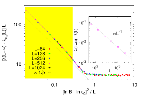
Scaling relations (14) and (16) can be cast into

$$\lambda(L=\infty)-\lambda_{\varepsilon_{0}}(L)=f(\rho)/L$$ (17)

where $\rho=(\ln B-\ln\varepsilon_{0})^{2}/L$ and $f(\rho)$ is a scaling function: For $\rho\gg 1$, $f(\rho)={\rm const.}$, as expected from (14); whereas for $\rho\ll 1$, $f(\rho)$ should scale as $\sim\rho^{-1}$, according to (16). Using the data from our simulations we can test the validity of this scaling law. Figure 2 shows a very good collapse with just one fitting parameter, $\ln B=2.2$, for different system sizes and values of $\varepsilon_{0}$. Our scaling argument is in good agreement with numerical data shown in Fig. 2, where one can see how the $\rho\ll 1$ asymptote converges to $1/\rho$ (shaded region in Fig. 2). However, the approximation appears to be too crude to describe the behavior very close to the crossover point $\rho\approx 1$, where the functional form of $f(\rho)$ deviates from the asymptote. Nonetheless the correct scaling variable $\rho$ for the scaling relation (17) and the two asymptotes are correctly captured. The crossover of $f(\rho)$ at $\rho\approx 1$ marks the departure from a regime dominated by the finite-size system effects to the dominance of the amplitude $\varepsilon_{0}$ of the Log-BV.

Figure 2: (color on line) Data collapse of $\lambda_{\varepsilon_{0}}(L)$, defined in (11) and (13), for different values of $\varepsilon_{0}$ and system size $L$ ($F=8$). Points fall approximately on a line, the scaling function $g$ in (17). Inset: The value of the LE $\lambda(L=\infty)$ was determined by extrapolating the largest LE from finite systems using (14)

V.2 Bred exponents vs. Lyapunov spectrum

In the preceding subsection we have introduced the concept of bred vector exponent $\lambda_{\varepsilon_{0}}$ as the growth rate for a Log-BV of amplitude $\varepsilon_{0}$. We have also seen how this BE approaches the leading LE in a finite size system as the amplitude $\varepsilon_{0}$ is varied. Now we devote the present subsection to study the connection of the BEs with the spectrum of LEs. The question we want to address is to what extent growth rates of Log-BVs (finite errors) approach growth rates of LVs (infinitesimal errors).

V.2.1 Main hypothesis

From the scaling arguments discussed above, it can be expected that the BE $\lambda_{\varepsilon_{0}}$ ought to be close to the $n$-th Lyapunov exponent $\lambda_{n}$ whenever both of them are piecewise copies of the leading Lyapunov vector with similar plateau sizes. This hypothesis reads more formally:

$$\lambda_{\varepsilon_{0}}\approx\lambda_{n}\;\;{\rm if}\;\;l_{c}^{BV}(\varepsilon_{0})\approx l_{c}^{LV}(n)\,,$$ (18)

where $l_{c}^{BV}$ ($l_{c}^{LV}$) indicates the typical length scale over which the Log-BV (the $n$-th LV) surface is a piecewise copy of the leading LV. In the following we will drop the superindices $BV$ and $LV$, as it is clear from the argument ($\varepsilon_{0}$ or $n$) what vector type we are referring to.

Figure 3: (color online) The lines with symbols are structure factors $S(k)$ obtained for Log-BVs with different perturbation amplitudes for $F=8.0$ and $L=1024$. The straight lines without symbols indicate the method of estimating the values $k_{c}(\varepsilon_{0})$ which are determined from the intersection of a horizontal line at $S(k_{min}=2\pi/L)$ and a power-law $S(k)\propto k^{-2.02}$ obtained from fitting the structure factor for $\min(\ln\varepsilon_{0})$.

V.2.2 Estimation of crossover wavenumbers $k_{c}(\varepsilon_{0})$

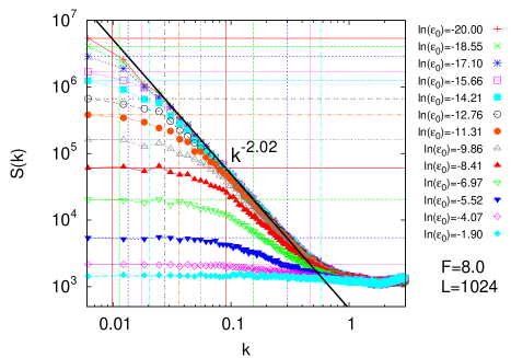
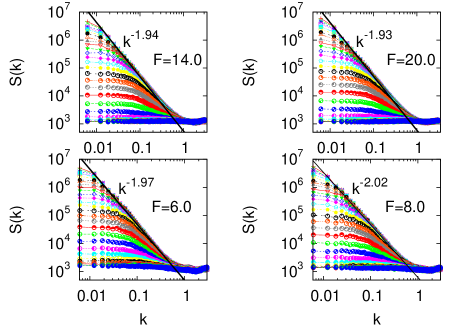
In Sec. IV.2 we showed that Log-BVs are piecewise copies of the main LV. This observation is now exploited to obtain a connection between BEs and LEs. In order to do so, we find it very convenient to look at the form of spatial correlations in Fourier space. The structure factors of Log-BV-surfaces with different values of $\varepsilon_{0}$ are presented in Fig. 3. As we have seen in Fig. 1 the Log-BV-surface follows the leading LV-surface at short scales and, as a consequence, their respective structure factors should overlap above a certain $k_{c}(\varepsilon_{0})$. This implies that both (Log-BV and LV) surface types share an interval $k_{c}(\varepsilon_{0})<k<\bar{k}\simeq 0.3$ with power-law structure factor $S(k)\sim k^{-2}$. Log-BVs exhibit flat structure factors for $k$ smaller than a certain $k_{c}(\varepsilon_{0})$, which indicates that distant regions (corresponding to small $k$) are basically uncorrelated. The crossover wavenumber $k_{c}(\varepsilon_{0})\sim l_{c}(\varepsilon_{0})^{-1}$ is monotonically increasing with $\varepsilon_{0}$ and, from Eq. (15), we have $k_{c}(\varepsilon_{0})\sim(\ln B-\ln\varepsilon_{0})^{-1/\alpha}$ with $\alpha=1/2$. Notably, surfaces associated with LVs for $n>1$ have a structure factor that also exhibits a knee at a certain crossover wavenumber $k_{c}(n)$ Szendro2007 ; Pazo2008 . In sum, structure factors of LV-surfaces and Log-BV-surfaces are very similar (cf. Fig. 4 in Pazo2010 ), and they only differ in the algebraic dependence below the particular crossover wavenumber $k_{c}$: $1/k$-type for the LVs, and flat ($k^{0}$) for the Log-BVs Pazo2010 , reflecting their different spatial correlations at large scales.

Figure 4: (color online) Collapse of the structure factors using the the values $k_{c}(\varepsilon_{0})$ determined from the structure factors $S(k)$ in Fig. 3.

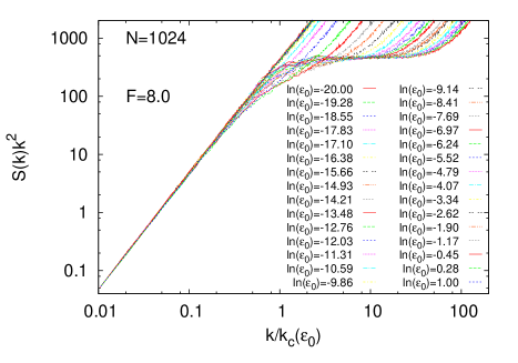
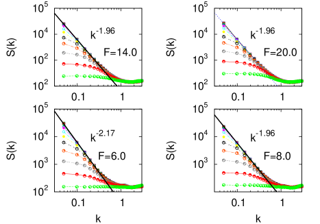
The crossover wavenumbers $k_{c}(\varepsilon_{0})$ of the Log-BV-surfaces $h_{\varepsilon_{0}}(x,t)$ can be systematically extracted from their structure factors $S(k)$, see Fig. 3 for $L=1024$ and $F=8$. Figure 4 shows the collapse of different structure factors when normalizing the wavenumbers by $k_{c}(\varepsilon_{0})$, giving an idea of the goodness of the estimation of $k_{c}(\varepsilon_{0})$. Figures 5 and 7 show that the same procedure can be used for other values of $F$ and smaller systems.

Figure 5: The lines with symbols indicate structure factors $S(k)$ obtained for bred vectors with different perturbation amplitudes with $F=6,8,14,20$ and $L=1024$. The values $k_{c}(\varepsilon_{0})$ are determined like in Fig. 3.

V.2.3 Numerical results

In extended systems, it is customary to represent LEs with the index $n$ normalized by the system size (or by the number of degrees of freedom). This is done so to highlight the extensivity (assuming it exists) of the model because LEs for different systems sizes with identical parameter values will approximately fall on the same line. Figure 6 shows the LEs connected by black lines. The Lyapunov spectra were obtained using the standard algorithm by Benettin et al. Benettin1980-1 ; Benettin1980-2 ; Wolf1985 .

Figure 6: (color online) Lyapunov spectra (solid black lines) and bred exponents (symbols). Size $L=1024$, and $F=6,7,\ldots,20$.

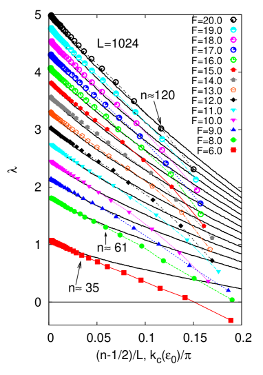
We found in Ref. Szendro2007 for an extensive coupled map lattice that $k_{c}(n)\sim(n/L)^{\theta}$, with $\theta$ around one. This means that representing the LEs versus $(n/L)$ is, for moderate values of $n$, equivalent to use a quantity proportional to $k_{c}(n)$ in the $x$-axis.

If now we want to test our hypothesis that BEs and LEs are similar if the crossover length scales coincide, we have to normalize $k_{c}(\varepsilon_{0})$ to use it as an independent variable in the range $(0,1)$. This normalization yields $k_{c}(\varepsilon_{0})/\pi$, and we may see in Fig. 6 that indeed BEs and LEs fall very near in the first part of the Lyapunov spectrum. This range of approximate overlapping is limited by the value of $n$ (or $\varepsilon_{0}$) up to which the LVs (or the Log-BVs) are piecewise copies of the main LV. Note also that this range expands as $F$ increases and the system becomes more chaotic.

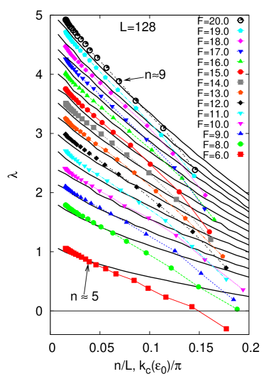
Figures 7 and 8 show that the same procedure can be followed also for a smaller system size ($L=128$). Note that as the system is extensive the figures look very much the same as those for $L=1024$.

Figure 7: (color online) The colored lines with symbols indicate structure factors $S(k)$ obtained for Log-BVs with different perturbation amplitudes for $F=6,8,14,20$ and $L=128$. The values $k_{c}(\varepsilon_{0})$ are determined like in Fig. 3

Figure 8: (color online) Lyapunov spectra (solid black lines) and bred exponents (symbols). Size $L=128$, and $F=6,7,\ldots,20$.

VI Conclusions

Although dynamical systems theory can characterize essentially all the properties of a chaotic system in terms of the properties of the tangent space directions (LVs) and their associated growth rates, the use of these linear analysis tools in real applications is often restricted by practical limits. This is particularly obvious in atmospheric dynamics and weather prediction systems were operative models include mathematical subtleties like ad-hoc parametrizations of many physical processes, nondifferentiable structures, and discrete programming structures that render the model unsuitable for linearization. In this context, much insight has been achieved by studying finite amplitude and truly nonlinear perturbations. In particular BVs have attracted much attention as a tool to investigate propagation of errors in both toy and operative weather models. However, little was known about the relation of finite BVs and truly infinitesimal LVs, apart from the obvious fact that a BV should tend to be collinear with the leading LV as the BV amplitude $\varepsilon_{0}$ tends to zero (independently of the norm definition used).

In this paper we have uncovered a number of connections between bred and Lyapunov vectors, which are specially noticeable and most conveniently characterized when one uses the zero-norm BVs or Log-BVs. We have also found that these similarities appear over a spatial range, below some characteristic length scale, that depends on the BVs amplitude. After a Hopf-Cole transformation, the Log-BVs turn out to be a piecewise copy of the leading LV. This resembles what has been previously reported for non-leading LVs Szendro2007 ; Pazo2008 . Interestingly, the spatial structure of Log-BVs shows clearly that they are uncorrelated objects at long length scales over certain characteristic length. This contrasts with LVs that were shown to exhibit weak correlations (decaying as $1/k$ with the wavenumber) at long scales Szendro2007 ; Pazo2008 . This immediately implies that the relative heights of the plateaus relating Log-BVs and the LV are not constrained by the dynamics. In turn different initial conditions yield a diversity of Log-BVs but nonetheless similar local patterns. Interestingly, this “regional” coincidence was observed before in bred vectors of a global circulation model of the atmosphere TothKalnay1997 , but remained up to now unexplained. Here we have shown that this regional similarities of BVs of different amplitudes $\varepsilon_{0}$ may be understood as due to the overlapping with the leading LV below a certain spatial range.

This paper has also investigated the relation between the growth rate of Log-BVs (the BEs) and the LEs. We have introduced the concept of bred exponents that describe how nonlinear perturbations grow in time. We have found that BEs and LEs can be mapped onto each other when the crossover length scales of the corresponding vector perturbations coincide. This is only true for the most expanding (bred or Lyapunov) exponents, when the “piecewise KPZ” picture holds. The convergence of the BE (a finite-time LE) to the largest LE has been found to follow a generic scaling function, which has been explained by a simple argument.

Finally, it is to be emphasized that we have used the Lorenz ’96 model in our simulations, but very similar results should be expected for other dissipative systems with spatiotemporal chaos.