Relic gravitational waves in the light of 7-year Wilkinson Microwave Anisotropy Probe data and improved prospects for the Planck mission

Abstract

The new release of data from Wilkinson Microwave Anisotropy Probe improves the observational status of relic gravitational waves. The 7-year results enhance the indications of relic gravitational waves in the existing data and change to the better the prospects of confident detection of relic gravitational waves by the currently operating Planck satellite. We apply to WMAP7 data the same methods of analysis that we used earlier [W. Zhao, D. Baskaran, and L.P. Grishchuk, Phys. Rev. D 80, 083005 (2009)] with WMAP5 data. We also revised by the same methods our previous analysis of WMAP3 data. It follows from the examination of consecutive WMAP data releases that the maximum likelihood value of the quadrupole ratio $R$, which characterizes the amount of relic gravitational waves, increases up to $R=0.264$, and the interval separating this value from the point $R=0$ (the hypothesis of no gravitational waves) increases up to a $2\sigma$ level. The primordial spectra of density perturbations and gravitational waves remain blue in the relevant interval of wavelengths, but the spectral indices increase up to $n_{s}=1.111$ and $n_{t}=0.111$. Assuming that the maximum likelihood estimates of the perturbation parameters that we found from WMAP7 data are the true values of the parameters, we find that the signal-to-noise ratio $S/N$ for the detection of relic gravitational waves by the Planck experiment increases up to $S/N=4.04$, even under pessimistic assumptions with regard to residual foreground contamination and instrumental noises. We comment on theoretical frameworks that, in the case of success, will be accepted or decisively rejected by the Planck observations.

I Introduction

The Wilkinson Microwave Anisotropy Probe (WMAP) Collaboration has released the results of 7-year (WMAP7) observations wmap7 ; wmap7-larson . In this paper, we apply to WMAP7 data the same methods of analysis that we have used before stable in the analysis of WMAP5 data. This is important for updating the present observational status of relic gravitational waves and for making more accurate forecasts for the currently operating Planck mission planck .

In Sec. II we briefly summarize our basic theoretical foundations and working tools. Part of this material was present in the previous publication stable , but in order to make the paper self-contained we briefly repeat it here. Section III exposes full details of our maximum likelihood analysis of WMAP7 data. In the focus of attention is the interval of multipoles $2\leq\ell\leq 100$, where gravitational waves compete with density perturbations. We compare all the results that we derived by exactly the same method from WMAP7, WMAP5 and WMAP3 datasets. This comparison demonstrates the stability of data and data analysis. On the grounds of this comparison, one can say that the perturbation parameters found from the consecutive WMAP data releases have the tendency of saturating near some particular values. The WMAP7 maximum likelihood (ML) value of the quadrupole ratio $R$ is close to previous evaluations of $R$, but increases up to $R=0.264$. The interval separating this ML value from the point $R=0$ (the hypothesis of no gravitational waves) increases up to a $2\sigma$ level. The primordial spectra remain blue, but the spectral indices in the relevant interval of wavelengths increase up to $n_{s}=1.111$ and $n_{t}=0.111$.

In Sec. IV we analyze why, to what extent, and in what sense our conclusions with respect to relic gravitational waves differ from those reached by the WMAP Collaboration. The WMAP team has found “no evidence for tensor modes.” A particularly important issue, which we discuss in some detail, is the presumed constancy (or simple running) of spectral indices. We derive an exact formula for the spectral index $n_{t}$ as a function of wavenumbers and discuss in this context the formula for running that was used in WMAP analysis. Another contributing factor to the difference of conclusions is the difference in our treatments of the inflationary “consistency relations” based on the inflationary “classic result.” We do not use the inflationary theory.

A comprehensive forecast for Planck findings in the area of relic gravitational waves is presented in Sec. V. We discuss the efficiency of various information channels, i.e. various correlation functions and their combinations. We perform multipole decomposition of the calculated $S/N$ and discuss physical implications of the detection in various intervals of multipole moments. We stress again that the $B$-mode detection provides the most of $S/N$ only in the conditions of very deep cleaning of foregrounds and relatively small values of $R$. The improvements arising from a 28-month, instead of a nominal 14-month, Planck survey are also discussed. In the center of our attention is the model with the WMAP7 maximum likelihood set of parameters. For this model, the signal-to-noise ratio $S/N$ in the detection of relic gravitational waves by Planck experiment increases up to $S/N=4.04$, even under pessimistic assumptions with regard to residual foreground contamination and instrumental noises. Section VI gives Bayesian comparison of different theoretical frameworks and identifies predictions of $R$ that may be decisively rejected by the Planck observations.

II Perturbation parameters and CMB power spectra

The temperature and polarization anisotropies of CMB are produced by density perturbations, rotational perturbations and gravitational waves. Rotational perturbations are expected to be very small and are usually ignored, and are in this paper, too. The cosmological perturbations are characterized by their gravitational field (metric) power spectra which are in general functions of time. Here, we introduce the notations and equations that will be used in subsequent calculations.

As before (see stable , mg12 , and references therein), we are working with perturbed Friedmann-Lemaitre-Robertson-Walker universes

$$ds^{2}=-c^{2}dt^{2}+a^{2}(t)(\delta_{ij}+h_{ij})dx^{i}dx^{j}=a^{2}(\eta)[-d\eta^{2}+(\delta_{ij}+h_{ij})dx^{i}dx^{j}],$$

where the functions $h_{ij}(\eta,{\bf x})$ are metric perturbation fields. Their spatial Fourier expansions are given by

$$h_{ij}(\eta,{\bf x})=\frac{\mathcal{C}}{(2\pi)^{3/2}}\int_{-\infty}^{+\infty}\frac{d^{3}{\bf n}}{\sqrt{2n}}\sum_{s=1,2}\left[\stackrel{{\scriptstyle s}}{{p}}_{ij}({\bf n})\stackrel{{\scriptstyle s}}{{h}}_{n}(\eta)e^{i{\bf n}\cdot{\bf x}}\stackrel{{\scriptstyle s}}{{c}}_{\bf n}+\stackrel{{\scriptstyle s~{}*}}{{p_{ij}}}({\bf n})\stackrel{{\scriptstyle s~{}*}}{{h_{n}}}(\eta)e^{-i{\bf n}\cdot{\bf x}}\stackrel{{\scriptstyle s~{}{\dagger}}}{{c_{\bf n}}}\right].$$ (1)

The polarization tensors $\stackrel{{\scriptstyle s}}{{p}}_{ij}({\bf n})$ ($s=1,2$) refer either to the two transverse-traceless components of gravitational waves (gw) or to the scalar and longitudinal-longitudinal components of density perturbations (dp). Density perturbations necessarily include perturbations of the accompanying matter fields (not shown here).

In the quantum version of the theory, the quantities $\stackrel{{\scriptstyle s}}{{c}}_{\bf n}$ and $\stackrel{{\scriptstyle s~{}{\dagger}}}{{c_{\bf n}}}$ are the annihilation and creation operators, respectively, of the considered type of perturbations, and the $|0\rangle$ is the initial vacuum (ground) state of the corresponding time-dependent Hamiltonian. The metric power spectrum $h^{2}(n,\eta)$ is defined by the expectation value of the quadratic combination of the metric field:

$$\langle 0|h_{ij}(\eta,{\bf x})h^{ij}(\eta,{\bf x})|0\rangle=\int\limits_{0}^{\infty}\frac{dn}{n}~{}h^{2}(n,\eta),~{}~{}~{}~{}~{}h^{2}(n,\eta)\equiv\frac{\mathcal{C}^{2}}{2\pi^{2}}n^{2}\sum_{s=1,2}|\stackrel{{\scriptstyle s}}{{h}}_{n}(\eta)|^{2}.$$ (2)

The mode functions $\stackrel{{\scriptstyle s}}{{h}}_{n}(\eta)$ are taken either from gw or dp equations, and $\mathcal{C}=\sqrt{16\pi}l_{\rm Pl}$ for gravitational waves and $\mathcal{C}=\sqrt{24\pi}l_{\rm Pl}$ for density perturbations.

The simplest assumption about the initial stage of cosmological expansion (i.e. about the initial kick that presumably took place soon after the birth of our Universe zg ; gr09 ) is that it can be described by a single power-law scale factor gr74 ; disca ; gr09

$$a(\eta)=l_{o}|\eta|^{1+\beta},$$ (3)

where $l_{o}$ and $\beta$ are constants, $\beta<-1$. Then the generated primordial power spectra (primordial means the interval of the spectrum pertaining to wavelengths longer than the Hubble radius at the considered moment of time) have the universal power-law dependence, both for gw and dp:

$$h^{2}(n)\propto n^{2(\beta+2)}.$$

It is common to write these power spectra separately for gw and dp:

$$h^{2}(n)~{}({\rm gw})=B_{t}^{2}n^{n_{t}},~{}~{}~{}~{}~{}h^{2}(n)~{}({\rm dp})=B_{s}^{2}n^{n_{s}-1}.$$ (4)

In accordance with the theory of quantum-mechanical generation of cosmological perturbations gr74 ; disca ; gr09 , the spectral indices are approximately equal $n_{s}-1=n_{t}=2(\beta+2)$ and the amplitudes $B_{t}$ and $B_{s}$ are of the order of magnitude of the ratio $H_{i}/H_{\rm Pl}$, where $H_{i}\sim c/l_{o}$ is the characteristic value of the Hubble parameter during the kick.

If the initial stage of expansion is not assumed to be a pure power-law evolution (3), the spectral indices $n_{t}$ and $n_{s}-1$ are not constants, but their wavenumber dependence is calculable from the time dependence of the scale factor $a(\eta)$ and its time derivatives grsol . In fact, as we shall argue below, the CMB data suggest that even at a span of 2 orders of magnitude in terms of wavelengths the spectral index $n_{s}$ is not the same. We discuss this issue in detail in Sec. IV.

In what follows, we use the numerical code CAMB CAMB and related notations for gw and dp power spectra adopted there:

$$P_{t}(k)=A_{t}\left(\frac{k}{k_{0}}\right)^{n_{t}},~{}~{}~{}P_{s}(k)=A_{s}\left(\frac{k}{k_{0}}\right)^{n_{s}-1},$$ (5)

where $k_{0}=0.002$Mpc^-1. Technically, the power spectrum $P_{s}(k)$ refers to the curvature perturbation called $\mathcal{R}$ or $\zeta$, but the amplitudes $B_{s}$ and $(A_{s})^{1/2}$ are equal to each other up to a numerical coefficient of order 1. The constant dimensionless wavenumber $n$ is related to the dimensionful $k$ by $k=n/(2l_{H})$, where $l_{H}=c/H_{0}$ is the present-day Hubble radius. The wavenumber $n=n_{H}=4\pi$ marks the wavelength equal to $l_{H}$ today. The CMB temperature anisotropy at the multipole $\ell$ is mostly generated by metric perturbations with wavenumbers $n\approx\ell$ (see zbg for details). Setting $h=0.704$ we obtain $\ell\approx(0.85\times 10^{4}$Mpc$)k$, which is consistent with the numerical result $\ell\approx(1.0\times 10^{4}$Mpc$)k$ derived in zb .

The CMB temperature and polarization anisotropies are usually characterized by the four angular power spectra: $C_{\ell}^{TT}$, $C_{\ell}^{EE}$, $C_{\ell}^{BB}$, and $C_{\ell}^{TE}$ as functions of the multipole $\ell$. The contribution of gravitational waves to these power spectra has been studied, both analytically and numerically, in a number of papers Polnarev1 ; a8 ; a11 ; a12 ; a13 . The derivation of today’s CMB power spectra brings us to approximate formulas of the following structure a12 :

$$\begin{array}[]{l}C_{\ell}^{TT}=\int\frac{dn}{n}h^{2}(n,\eta_{rec})\left[F^{T}_{\ell}(n)\right]^{2},\\ C_{\ell}^{TE}=\int\frac{dn}{n}h(n,\eta_{rec})h^{\prime}(n,\eta_{rec})\left[F^{T}_{\ell}(n)F^{E}_{\ell}(n)\right],\\ C_{\ell}^{YY}=\int\frac{dn}{n}(h^{\prime})^{2}(n,\eta_{rec})\left[F^{Y}_{\ell}(n)\right]^{2},~{}~{}~{}~{}{\rm where}~{}Y=E,B.\end{array}$$ (9)

In the above expressions, $h^{2}(n,\eta_{rec})$ and $(h^{\prime})^{2}(n,\eta_{rec}$) are the power spectra of the gravitational wave field and its first time-derivative, respectively. The spectra are taken at the recombination (decoupling) time $\eta_{rec}$. The functions $F^{X}_{\ell}(n)$ ($X=T,E,B$) take care of the radiative transfer of CMB photons in the presence of metric perturbations. As already mentioned, the power residing in the metric fluctuations at wavenumber $n$ mostly translates into the CMB $TT$ power at the angular scales $\ell\approx n$. Similar results hold for the CMB power spectra induced by density perturbations. The actually performed numerical calculations use equations more accurate than Eq. (9). They also include the effects of the reionization era.

The CMB power spectra needed for the analysis of WMAP data are calculated in the framework of background cosmological $\Lambda$CDM model characterized by the WMAP7 best-fit parameters wmap7

$$\begin{array}[]{c}\Omega_{b}h^{2}=0.02260,~{}~{}~{}\Omega_{c}h^{2}=0.1123,~{}~{}~{}\Omega_{\Lambda}=0.728,~{}~{}~{}\tau_{\rm reion}=0.087,~{}~{}~{}h=0.704.\end{array}$$ (11)

To quantify the contribution of relic gravitational waves to the CMB we use the quadrupole ratio $R$ defined by

$$R\equiv\frac{C_{\ell=2}^{TT}({\rm gw})}{C_{\ell=2}^{TT}({\rm dp})}.$$ (12)

Another measure is the so-called tensor-to-scalar ratio $r$. This quantity is constructed from the primordial power spectra (5)

$$r\equiv\frac{A_{t}}{A_{s}}.$$ (13)

Often this parameter is linked to incorrect (inflationary) statements, such as the inflationary ‘consistency relation’ (more details in Sec. IV). However, if one uses $r$ without implying inflationary claims, one can find a useful relation between $R$ and $r$.

In general, the relation between $R$ and $r$ depends on background cosmological parameters and spectral indices $n_{s}$ and $n_{t}$. We found this relation numerically using the CAMB code CAMB . (For a semianalytical approach see rRrelation .) The results are plotted in Fig. 1. For this calculation we used the background cosmological parameters (11) and the condition $n_{t}=n_{s}-1$ required by the theory of quantum-mechanical generation of cosmological perturbations. We verified that the relation $r(R)$ only weakly depends on the background parameters and does not change significantly when the values (11) are varied within the WMAP7 $1\sigma$ error range wmap7 . It is seen from the graph that $r=1.92R$ in the case of $n_{s}=1.0$, and $r\approx 2R$ for all considered $n_{s}$, if $R$ and $r$ are sufficiently small. In other words, one can use $r\approx 2R$ for a quite wide class of models.

We do not know enough about the very early Universe to predict $R$ with any certainty. However, since the theory of quantum-mechanical generation of cosmological perturbations requires that the amplitudes $B_{t}$ and $B_{s}$ (as well as $A_{t}$ and $A_{s}$ in Eq.(5)) should be of the same order of magnitude, our educated guess is that $R$ should lie somewhere in the range $R\in[0.01,1]$. If $R$ were observationally found significantly outside this range, we would have to conclude that the underlying perturbations are unlikely to be of quantum-mechanical origin. On the other hand, the most advanced inflationary theories predict the ridiculously small amounts of gravitational waves, something at the level of $r\approx 10^{-24}$ or less, $r\in[0,10^{-24}]$. The rapidly improving CMB data will soon allow one to decisively discriminate between these theoretical frameworks (let alone the already performed discrimination on the grounds of purely theoretical consistency). We discuss this issue in Sec. VI.

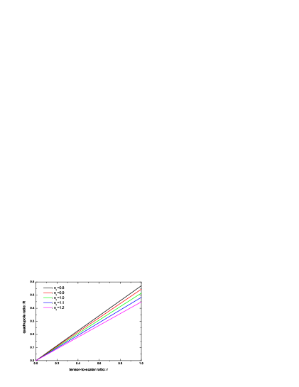
Figure 1: The relation between $R$ and $r$ for different values of the spectral index $n_{s}$. From top to bottom the $n_{s}$ changes from $n_{s}=0.8$ to $n_{s}=1.2$.

III Evaluation of relic gravitational waves from 7-year WMAP data

III.1 Likelihood function

Relic gravitational waves compete with density perturbations in generating CMB temperature and polarization anisotropies at relatively low multipoles. For this reason we focus on the WMAP7 data at $2\leq\ell\leq 100$. As before zbg ; stable , the quantities $D_{\ell}^{TT}$, $D_{\ell}^{TE}$, $D_{\ell}^{EE}$, and $D_{\ell}^{BB}$ denote the estimators (and also the actual observed data points in the likelihood analysis) of the corresponding power spectra. Since the WMAP7 $EE$ and $BB$ observations are not particularly informative, we marginalize (integrate) the total probability density function (pdf) over the variables $D_{\ell}^{EE}$ and $D_{\ell}^{BB}$ zbg ; stable . The resulting pdf stable is a function of $D_{\ell}^{TT}$ and $D_{\ell}^{TE}$:

$$f(D_{\ell}^{TT},D_{\ell}^{TE})=n^{2}{x}^{\frac{n-3}{2}}\left\{2^{1+n}\pi\Gamma^{2}(\frac{n}{2})(1-\rho_{\ell}^{2})(\sigma_{\ell}^{T})^{2n}(\sigma_{\ell}^{E})^{2}\right\}^{-\frac{1}{2}}$$

$$\times\exp\left\{\frac{1}{1-\rho^{2}_{\ell}}\left(\frac{{\rho_{\ell}}{z}}{{\sigma_{\ell}^{T}}{\sigma_{\ell}^{E}}}-\frac{{z}^{2}}{2x{(\sigma_{\ell}^{E})^{2}}}-\frac{{x}}{2{(\sigma_{\ell}^{T})^{2}}}\right)\right\}.$$ (14)

This pdf contains the variables $D_{\ell}^{XX^{\prime}}$ ($XX^{\prime}=TT,TE$) through the quantities ${x}\equiv n(D_{\ell}^{TT}+N_{\ell}^{TT})$ and ${z}\equiv nD_{\ell}^{TE}$, where $N_{\ell}^{TT}$ and $N_{\ell}^{EE}$ are total noise power spectra. Information about the power spectra $C_{\ell}^{XX^{\prime}}$ is contained in the quantities ${\sigma_{\ell}^{T}}$, ${\sigma_{\ell}^{E}}$ and $\rho_{\ell}$ (see stable for details). The sought after parameters $A_{s}$, $A_{t}$, $n_{s}$, and $n_{t}$ enter the pdf through the $C_{\ell}^{XX^{\prime}}$. The quantity $n=(2\ell+1)f_{\rm sky}$ in (14) is the effective number of degrees of freedom at multipole $\ell$, where $f_{\rm sky}$ is the sky-cut factor.

In the WMAP7 data release the sky-cut factor is $f_{\rm sky}=0.783$ wmap7-larson , which is slightly smaller than $f_{\rm sky}=0.85$ used in WMAP5 data analysis stable . The smaller $f_{\rm sky}$ increases the uncertainties, but this disadvantage is more than compensated by the reduction of overall noises. Therefore, the error bars surrounding the WMAP7 data points are somewhat smaller than those for the WMAP5 data release. This fact, together with slightly shifted data points themselves, allows us to strengthen our conclusions (see below) about the presence of gravitational wave signal in the WMAP data.

We seek the perturbation parameters $R$, $A_{s}$ and $n_{s}$ ($n_{t}=n_{s}-1$) along the lines of our maximum likelihood analysis of WMAP5 data stable . The pdf (14) considered as a function of unknown $R$, $A_{s}$, and $n_{s}$ with known data points $D_{\ell}^{XX^{\prime}}$ is a likelihood function subject to maximization. For a set of observed multipoles $\ell=2,\cdot\cdot\cdot,\ell_{max}$, the likelihood function can be written as stable

$$-2\ln\mathcal{L}=\sum_{\ell}\left\{\frac{1}{1-\rho^{2}_{\ell}}\left(\frac{{z}^{2}}{x{(\sigma_{\ell}^{E})^{2}}}+\frac{{x}}{{(\sigma_{\ell}^{T})^{2}}}-\frac{{2\rho_{\ell}}{z}}{{\sigma_{\ell}^{T}}{\sigma_{\ell}^{E}}}\right)+\ln\left((1-\rho_{\ell}^{2})(\sigma_{\ell}^{T})^{2n}(\sigma_{\ell}^{E})^{2}\right)\right\}+C,$$ (15)

where the constant $C$ is chosen to make the maximum value of $\mathcal{L}$ equal to 1.

III.2 Results of the analysis of the WMAP7 data

The WMAP7 data points for $D_{\ell}^{TT}$ and $D_{\ell}^{TE}$ at multipoles $2\leq\ell\leq\ell_{max}=100$ were taken, with gratitude, from the Website LAMBDA . The 3-dimensional likelihood function (15) was probed by the Markov chain Monte Carlo method mcmc1 ; mcmc2 using 10,000 samples. The ML values of the three perturbation parameters $R$, $n_{s}$ and $A_{s}$ were found to be

$$R=0.264,~{}~{}~{}n_{s}=1.111,~{}~{}~{}A_{s}=1.832\times 10^{-9}$$ (16)

and $n_{t}=0.111$. In Fig. 2 we show the projection of the 10,000 sample points on the 2-dimensional planes $R-n_{s}$ and $R-A_{s}$. The color of an individual point signifies the value of the 3-dimensional likelihood of the corresponding sample. The projections of the maximum (16) are shown by a black $+$. (The value $R=0.264$ is equivalent to $r=0.550$.)

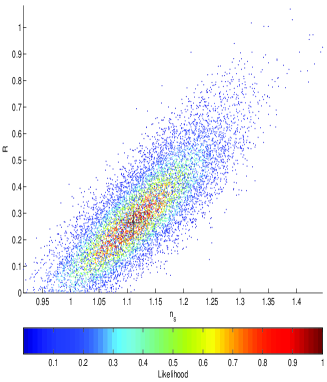
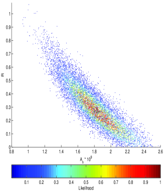
Figure 2: The projection of 10,000 samples of the 3-dimensional likelihood function, based on the WMAP7 data, onto the $R-n_{s}$ (left panel) and $R-A_{s}$ (right panel) planes. The black $+$ indicates the maximum likelihood parameters listed in (16).

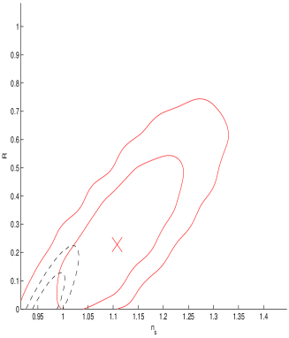
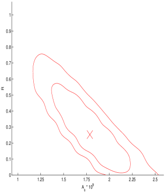
Figure 3: The ML point (red $\times$) and the $68.3\%$ and $95.4\%$ confidence intervals (red solid lines) for the 2-dimensional distributions $R-n_{s}$ (left panel) and $R-A_{s}$ (right panel). The left panel shows also the WMAP7 confidence contours (black dashed line) derived under the assumption that the spectral index $n_{s}$ is one and the same constant throughout all measured multipoles wmap7 ; wmap7-larson . The WMAP7 papers do not show the confidence contours in the $R-A_{s}$ plane.

Before analyzing the 3-parameter results, it is instructive to consider the 2-parameter and 1-parameter probability distributions of the sought after parameters. These marginalized distributions are obtained by integrating the likelihood function $\mathcal{L}$ (15) (already represented by 10,000 points) over one or two parameters. By integrating over $A_{s}$ or $n_{s}$, we arrive at 2-dimensional distributions for the pairs $R-n_{s}$ or $R-A_{s}$, respectively. The area around the maximum of the resulting distributions is shown in Fig. 3. In the $R-n_{s}$ space, the maximum is located at

$$R=0.228,~{}~{}~{}n_{s}=1.108.$$ (17)

In the $R-A_{s}$ space, the maximum is located at

$$R=0.253,~{}~{}~{}A_{s}=1.787\times 10^{-9}.$$ (18)

In the left panel we also reproduce the 2-dimensional contours obtained by the WMAP team wmap7 ; wmap7-larson (their $r$ is translated into our $R$). In contrast to the WMAP5 paper wmap5 , the WMAP7 paper wmap7-larson shows only the uncertainty contours derived under the assumption of a strictly constant spectral index $n_{s}$, but not for the case of its running.

The 1-dimensional distributions for $R$, $n_{s}$ or $A_{s}$ are obtained by integrating the likelihood function $\mathcal{L}$ (15) over the sets of two parameters ($A_{s}$, $n_{s}$), ($A_{s}$, $R$) or ($R$, $n_{s}$), respectively. These distributions are presented in Figs. 4 and  5 (red solid lines). The ML values of the parameters and their $68.3\%$ confidence intervals are found to be

$$R=0.273^{+0.185}_{-0.156},~{}~{}n_{s}=1.112^{+0.089}_{-0.064},~{}~{}A_{s}=(1.765^{+0.279}_{-0.263})\times 10^{-9}.$$ (19)

For completeness and comparison (see Sec. III.3), we also show in Figs. 4 and  5 the 1-dimensional (1-D, for brevity) distributions derived by exactly the same procedure from WMAP5 and WMAP3 observations. Obviously, the WMAP5 curves are copies of the previously reported distributions stable ; the WMAP3 curves are explained in Sec. III.3.

The constancy of spectral indices is a matter of special discussion in Sec. IV. In preparation for this discussion, we report the results of our likelihood analysis of data in other intervals of multipole moments $\ell$, in addition to the interval $2\leq\ell\leq 100$ that resulted in the ML values (16). First, we analyzed the WMAP7 data in the interval $101\leq\ell\leq 220$. The $n_{s}$ coordinate of the maximum in 3-dimensional space $R,A_{s}$, and $n_{s}$ was found to be $n_{s}=0.951$. The 1-D marginalized distribution for $n_{s}$ gave the ML result

$$n_{s}=0.969^{+0.083}_{-0.063}~{}(68.3\%~{}{\rm C.L.}).$$ (20)

Second, we have done the same in the combined interval of multipoles $2\leq\ell\leq 220$. The maximum of 3-D likelihood lies at $n_{s}=1.003$, whereas the 1-D ML result is

$$n_{s}=1.021^{+0.043}_{-0.038}~{}(68.3\%~{}{\rm C.L.}).$$ (21)

The 1-D results allow one to make easier comparison of confidence intervals. As is seen from (19) and (20), the 1-D determinations of $n_{s}$ in the adjacent ranges $2\leq\ell\leq 100$ and $101\leq\ell\leq 220$ overlap, but only marginally, in their $1\sigma$ intervals. As expected, if $n_{s}$ is assumed constant in the entire range $2\leq\ell\leq 220$, its value (21) is intermediate between (19) and (20). The spreads of wavenumbers to which the 3-d spectral indices $n_{s}=1.111$, $n_{s}=0.951$ and $n_{s}=1.003$ refer are shown by marked red lines in Fig. 6.

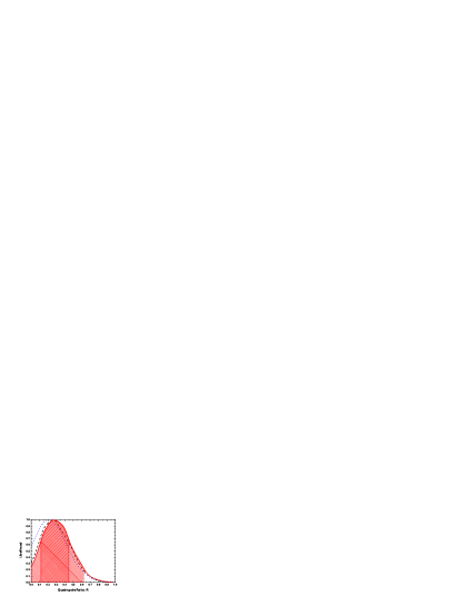
Figure 4: The 1-dimensional likelihoods for $R$. The results of the analysis of WMAP7, WMAP5 and WMAP3 data are shown, respectively, by the red (solid), black (dashed), and blue (dotted) curves. The shaded regions indicate the $68.3\%$ and $95.4\%$ confidence intervals for WMAP7 likelihood.

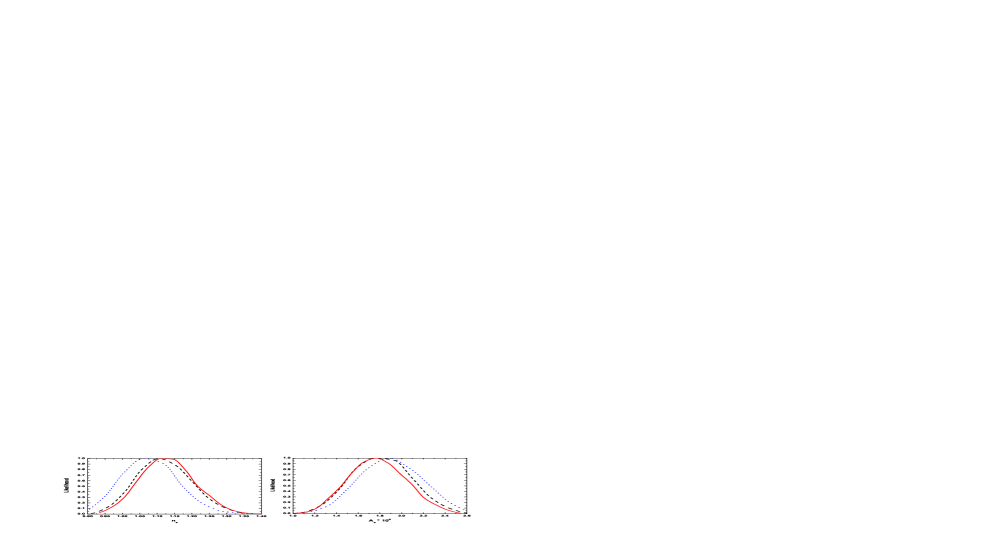
Figure 5: The 1-dimensional likelihoods for $n_{s}$ (left) and $A_{s}$ (right). In both panels the red (solid), black (dashed) and blue (dotted) curves show the results for WMAP7, WMAP5 and WMAP3 data, respectively.

III.3 Comparison of results derived from WMAP7, WMAP5 and WMAP3 data releases

One and the same 3-parameter analysis of WMAP5 and WMAP7 data has resulted in somewhat different ML parameters. From WMAP7 observations we extracted the ML parameters (16), whereas the ML parameters extracted from WMAP5 observations stable are

$$R=0.229,~{}~{}~{}n_{s}=1.086,~{}~{}~{}A_{s}=1.920\times 10^{-9}.$$

Certainly, the results are consistent and close to each other. The same holds true for marginalized 1-dimensional parameters and distributions shown in Figs. 4 and  5. This similarity of results testifies to the stability of data and data analysis. There exist, however, important trends in the sequence of ML parameters extracted from the progressively improving WMAP3, WMAP5, and WMAP7 data. We want to discuss these trends.

Specially for this discussion, we derived the parameters $R,n_{s}$, and $A_{s}$ from WMAP3 data in exactly the same manner as was done here and in stable with WMAP7 and WMAP5 data releases. Previously zbg , we derived these parameters by a different method: we restricted the likelihood analysis to $TE$ data and a single parameter $R$, while $n_{s}$ and $A_{s}$ were determined from phenomenological relations designed to fit the $TT$ data. That analysis has led us to $R=0.149^{+0.247}_{-0.149}$ and $n_{s}=1.002$. Our new derivation, based on 3-dimensional likelihood, gives the following WMAP3 maximum likelihood parameters:

$$R=0.181,~{}~{}~{}n_{s}=1.045,~{}~{}~{}A_{s}=2.021\times 10^{-9}.$$

The corresponding 1-dimensional distributions give

$$R=0.205^{+0.181}_{-0.157},~{}~{}n_{s}=1.059^{+0.097}_{-0.066},~{}~{}A_{s}=(1.894^{+0.290}_{-0.307})\times 10^{-9}.$$ (22)

The 1-dimensional WMAP3 distributions are plotted in Figs. 4 and  5 by dotted curves alongside with WMAP5 (dashed) and WMAP7 (solid) curves.

Looking at all derivations and graphs collectively, we can draw the following conclusions. First, about $R$. The maximum likelihood value of $R$ increases as one goes over from 3-year to better quality 7-year data. The ML value $R=0.264$ of WMAP7 data release is $15\%$ larger than the analogous result $R=0.229$ obtained from WMAP5 data. The 3-, 2-, and 1-parameter determinations of $R$ persistently concentrate somewhere around the mark $R=0.25$. The uncertainties $\Delta R$, although still considerable, get smaller as one progresses from 3-year to better quality 7-year data. The $R=0$ (no gravitational waves) hypothesis is under increasing pressure. For example, the WMAP7 1-parameter result, Eq.(19) and Fig. 4, excludes the $R=0$ hypothesis at almost $2\sigma$ level. To be more precise, the $R=0$ point is right on the boundary of the $94\%$ confidence area ($94\%$ of surface area under the WMAP7 curve in Fig. 4) surrounding the 1-D ML value $R=0.273$. This is an improvement in comparison with a slightly larger than $1\sigma$ interval separating $R=0$ from the WMAP5 1-d ML value $R=0.266$ stable . Admittedly, the gradual changes in ML values of $R$ are small, while uncertainties are still large. It would not be very surprising if random realizations of noise moved the consecutive 3-year, 5-year, 7-year ML values of $R$ in arbitrary order. Nevertheless, we observe the tendency for systematic increase and saturation of $R$ alongside with decrease of $\Delta R$.

Second, our conclusions about $n_{s}$. Together with the increase of ML $R$, we observe the tendency for the increase of $n_{s}$ accompanied by the theoretically expected and understood decrease of $A_{s}$ (the contribution of relic gravitational waves becomes larger, while the contribution of density perturbations becomes smaller). The ML value $n_{s}=1.111$ derived from the WMAP7 data, Eq.(16), is larger than $n_{s}=1.086$ derived from WMAP5 data, while the WMAP7 value of $A_{s}$ is somewhat smaller than that of WMAP5 stable . The tendency for increase of $n_{s}$ and decrease of $A_{s}$ is also illustrated by the 1-parameter distributions in Fig. 5. The spectral indices $n_{s},n_{t}$ persistently point out to blue primordial spectra, i.e. $n_{s}>1$ for density perturbations and $n_{t}>0$ for gravitational waves, in the interval of wavelengths responsible for CMB anisotropies at $2\leq\ell\leq 100$. The larger values of $n_{s},~{}n_{t}$ derived from WMAP7 data release enhance the doubt on whether the conventional scalar fields could be the driver of the initial kick, since these cannot support $\beta>-2$ in Eq.(3) and, consequently, $n_{s}>1,~{}n_{t}>0$ in Eq.(4). (Since the inflationary theory is capable of predicting virtually anything that one can possibly imagine, there exist of course literature claiming that inflation can predict blue spectra. But these claims are based on the incorrect (inflationary) formula for density perturbations, see disca .) The questions pertaining to the spectral indices are analyzed in some detail in the next section.

IV Comparison of our results with conclusions of WMAP collaboration

Having analyzed the 7-year data release, the WMAP collaboration concludes that a minimal cosmological model without gravitational waves and with a constant spectral index $n_{s}$ across the entire interval of considered wavelengths remains a “remarkably good fit” to ever improving CMB data and other datasets. The WMAP team emphasizes: “We do not detect gravitational waves from inflation with 7-year WMAP data, however the upper limits are $16\%$ lower…” wmap7-larson , p.11; “The 7-year WMAP data combined with BAO and ${\rm H_{0}}$ excludes the scale-invariant spectrum by more than $3\sigma$, if we ignore tensor modes (gravitational waves)” wmap7 , p.15; “We find no evidence for tensor modes…” wmap7 , p.30; “We find no convincing deviations from the minimal model” wmap7 , p.1, etc.

In contrast, our analysis of WMAP3, WMAP5 and WMAP7 data leads us in the opposite direction: the improving data make the gw indications stronger. The major points of tension between the two approaches seem to be the constancy of spectral indices and the continuing use by the WMAP team of the inflationary theory in data analysis and interpretation. We shall start from the discussion of spectral indices.

The constancy of spectral indices is a reasonable assumption, but not a rule. If the power-law dependence (3) is not a good approximation to the gravitational pump field during some interval of time, the constancy of $n_{t},~{}n_{s}$ is not a good approximation to the generated primordial spectra (4) in the corresponding interval of wavelengths. In fact, the future measurements of frequency dependence of the spectrum of relic gravitational waves will probably be the best way to infer the “early history of the Hubble parameter” grsol .

The frequency-dependence of a gw spectrum is fully determined by the time-dependence of the function $\gamma(t)\equiv-{\dot{H}}/{H^{2}}$. (In more recent papers of other authors this function is often denoted $\epsilon(t)$.) The function $\gamma(t)$ describes the rate of change of the time-dependent Hubble radius $l_{H}(t)\equiv c/H(t)$:

$$\gamma(t)=\frac{d}{dt}\left(\frac{1}{H(t)}\right)=\frac{1}{c}\frac{dl_{H}(t)}{dt}.$$

The function $\gamma(t)$ is a constant for power-law scale factors (3): $\gamma=(2+\beta)/(1+\beta)$, and $\gamma=0$ for a period of de Sitter expansion. The interval of time $dt$ during the early era when gravitational waves were entering the amplifying regime and their today’s frequency spread $d\nu$ are related by (see Eq.(21) in grsol ):

$$\frac{d}{dt}=[1-\gamma(\nu)]H(\nu)\frac{d}{d\ln\nu}.$$

The today’s spectral energy density of gravitational waves $\epsilon(\nu)$ is related to the early universe parameter $\gamma(t)$ by (see Eq.(22) in grsol ):

$$\gamma(\nu)=-\frac{[d~{}\ln\epsilon(\nu)/d~{}\ln\nu]}{2-[d~{}\ln\epsilon(\nu)/d~{}\ln\nu]}.$$ (23)

The spectral index $n_{g}$ of a pure power-law energy density $\epsilon(\nu)\propto\nu^{n_{g}}$ is defined as $n_{g}=[d~{}\ln\epsilon(\nu)/d~{}\ln\nu]$. It is reasonable to retain this definition for more complicated spectra. Then, Eq.(23) can be rewritten as

$$n_{g}(\nu)=-\frac{2\gamma(\nu)}{1-\gamma(\nu)}.$$ (24)

Obviously, in the case of pure power-laws (3) we return to the constant spectral index $n_{g}=-2\gamma/(1-\gamma)=2(2+\beta)$.

Equation (24) was derived for the energy density of relatively high-frequency gravitational waves, $\nu>10^{-16}{\rm Hz}$, which started the adiabatic regime during the radiation-dominated era. In our CMB study we deal with significantly lower frequencies. It is more appropriate to speak about wavenumbers $n$ rather than frequencies $\nu$, and about power spectra of metric perturbations $h^{2}(n)$ rather than energy density $\epsilon(\nu)$. The $k$-dependent spectral index $n_{t}(k)$ entering primordial spectrum (5) is defined as $n_{t}(k)=[d~{}\ln P_{t}(k)/d~{}\ln k]$. Then formula for $n_{t}(k)$ retains exactly the same appearance as Eq.(24):

$$n_{t}(k)=-\frac{2\gamma(k)}{1-\gamma(k)}.$$ (25)

The spectral index $n_{t}(k)$ reduces to a constant $n_{t}=2(2+\beta)$ in the case of power-law functions (3).

The spectral index $n_{s}(k)-1$ for density perturbations is defined by $n_{s}(k)-1=[d~{}\ln P_{s}(k)/d~{}\ln k]$. The formula for $n_{s}(k)-1$ is more complicated than Eq.(25) as it contains also $d\gamma(t)/dt$ as a function of $k$. However, it is important to stress that adjacent intervals of power-law evolution (3) with slightly different constants $\beta$, will result in slightly different pairs of constant indices $n_{t},~{}n_{s}-1$ in the corresponding adjacent intervals of wavelengths. Of course, the spectrum itself is continues at the wavelength marking the transition between the two regions.

Extending the minimal model, the WMAP Collaboration works with the power spectrum wmap7

$$P_{s}(k)=P_{s}(k_{0})\left(\frac{k}{k_{0}}\right)^{n_{s}(k_{0})-1+\frac{1}{2}\alpha_{s}\ln(k/k_{0})},$$ (26)

which means that the $k$-dependent (running) spectral index $n_{s}(k)$ is assumed to be a constant plus a logarithmic correction:

$$n_{s}(k)=n_{s}(k_{0})+\alpha_{s}\ln(k/k_{0}).$$ (27)

The aim of WMAP data analysis is to find $\alpha_{s}$, unless it is postulated from the very beginning, as is done in the central (minimal) model, that $\alpha_{s}\equiv 0$. We note that although logarithmic corrections do arise in simple situations and can even be termed “natural” grsol , they are not unique or compulsory, as we illustrated by exact formula (25). Nevertheless, we do not debate this point. We accept WMAP’s definitions, and we want to illustrate their results graphically, together with our evaluations of $n_{s}$ in this paper.

The main result of WMAP7 determination is $n_{s}=0.963\pm 0.012$ (68% C.L.) derived under the assumption of no gravitational waves and constant $n_{s}$ throughout all wavelengths included in the considered datasets wmap7 ; wmap7-larson . When the presence of gravitational waves is allowed, but $n_{s}$ is still assumed constant, the $n_{s}$ rises to $n_{s}=0.982^{+0.020}_{-0.019}$ from WMAP7 data alone. Finally, from WMAP7 data alone, the WMAP team finds $n_{s}(k_{0})=1.027,~{}\alpha_{s}=-0.034$ in the case of no gw but with running of $n_{s}$, and $n_{s}(k_{0})=1.076,~{}\alpha_{s}=-0.048$ in the case of running and allowed gravitational waves (we quote only central values without error bars, see Table 7 in wmap7 ). All the resulting values of $n_{s}(k)$ derived by WMAP team are shown in Fig. 6. For comparison, we also plot by red lines our evaluations of $n_{s}$, see Sec. III.2.

The lines in Fig. 6 show clearly that our finding of a blue shape of the spectrum, i.e. $n_{s}=1.111$, at longest accessible wavelengths is pretty much in the territory of WMAP findings, if one allows running, even as simple as Eq.(27), and especially when running is combined with gravitational waves. On the other hand, as was already explained in stable , the attempt of constraining relic gravitational waves by using the data from a huge interval of wavelengths and assuming a constant $n_{s}$ (or its simple running) across all wavelengths is unwarranted. The high-$\ell$ CMB data, as well as other datasets at relatively short wavelengths, have nothing to do with relic gravitational waves, and their use is dangerous. As we argued in Sec. III.2, the spectral index $n_{s}$ appears to be sufficiently different even at the span of two adjacent intervals of wavenumbers. The restriction to a relatively small number of multipoles $2\leq\ell\leq 100$ is accompanied by relatively large uncertainties in $R$, but there is nothing we can do about it to improve the situation, this is in the nature of efforts aimed at measuring $R$. The difference in the treatment of $n_{s}$ is probably the main reason why we do see indications of relic gravitational waves in the data, whereas the WMAP team does not.

Another contributing factor to the difference of conclusions is the continuing use by WMAP Collaboration of the inflationary theory and its (incorrect) relation $n_{t}=-r/8$, which automatically sends $r$ to zero when $n_{t}$ approaches zero. This formula is a part of the inflationary ‘consistency relations’

$$r=16\epsilon=-8n_{t}.$$

Only one equality in this formula, $16\epsilon=-8n_{t}$, is correct being an approximate version (for small $\gamma$, $\epsilon\equiv\gamma$) of our exact formula, Eq. (25). The ‘consistency relation’ $r=16\epsilon$ is incorrect. It is an immediate consequence of the “classic result” of inflationary theory, namely, the prediction of arbitrarily large amplitudes of density perturbations generated in the limit of de Sitter inflation ($\epsilon=0,~{}n_{s}=1$), regardless of the strength of the generating gravitational field (curvature of space-time) regulated by the Hubble parameter $H$ . Certainly, it would be inconsistent, even by the standards of inflationary theory, not to use the relation $r=-8n_{t}$ in data analysis, if the inflationary “classics” is used in derivation of power spectra and interpretation of results (see, for example, Fig. 19 in wmap7 ). Obviously, in our analysis we do not use the inflationary theory and its relations.

Figure 6: The spectral index $n_{s}$ as a function of the wavenumber $k$. The ML results of this work are shown by red lines. Other lines are our plots of WMAP7 findings wmap7 , Table 7.

V Forecasts for the Planck mission based on the results of analysis of WMAP7 data

The Planck satellite planck is currently making CMB measurements and is expected to provide data of better quality than WMAP. We hope that the indications of relic gravitational waves that we found in WMAP3, WMAP5 and WMAP7 data will become a certainty after Planck observations. We quantify the detection ability of the Planck experiment by exploring the vicinity of the WMAP7 maximum likelihood parameters (16).

It is seen from Fig. 2 that the samples with relatively large values of the likelihood (red, yellow, and green) are concentrated along the curve which projects into relatively straight lines (at least, up to $R\approx 0.5$) in the planes $R-n_{s}$ and $R-A_{s}$:

$$n_{s}=0.98+0.49R,~{}~{}~{}~{}~{}A_{s}=(2.30-1.77R)\times 10^{-9}.$$ (28)

The ML model (16) is a specific point on these lines, corresponding to $R=0.264$. The parameterization (28) is close to the result derived from WMAP5 data: $n_{s}=0.98+0.46R,~{}A_{s}=(2.27-1.53R)\times 10^{-9}$, and ML $R=0.229$ (see Eq. (15) in stable ). We use Eq.(28) in formulating our forecast, thus reducing the task of forecasting to a 1-parameter problem in terms of $R$.

Following stable , we define the signal-to-noise ratio as

$$S/N\equiv R/\Delta R,$$ (29)

where the numerator is the true value of the parameter $R$ (or its ML value, or the input value in a numerical simulation) while $\Delta R$ in the denominator is the uncertainty in determination of $R$ from the data.

We estimate the uncertainty $\Delta R$ using the Fisher matrix formalism. We take into account all available information channels, i.e. $TT$, $TE$, $EE$ and $BB$ correlation functions, and their various combinations. The uncertainty $\Delta R$ depends on instrumental and environmental noises, on the statistical uncertainty of the CMB signal itself, and on whether other parameters, in addition to $R$, are derived from the same dataset. All our input assumptions about Planck’s instrumental noises, number and specification of frequency channels, foreground models and residual contamination, sky coverage and lifetime of the mission, etc. are exactly the same as in our previous paper stable . We do not repeat the details here and refer the reader to the text and appendices in stable which contain necessary references. Technically, our present forecast is somewhat different (better) than that in the previous analysis stable because of slightly different family of preferred perturbation parameters (28), with slightly higher than before the ML value of $R$, $R=0.264$. We have added only one new calculation, reported in Fig. 11 and Fig. 12, which is the $S/N$ for the survey of 28 months duration, instead of the nominal assumption of 14 months.

The results of our forecast for the Planck mission are presented in figures. In Fig. 7 we show the total $S/N$ for the case $TT+TE+EE+BB$, i.e. when all correlation functions are taken into account, and at all relevant multipoles $2\leq\ell\leq 100$. The possible levels of foreground cleaning are marked by $\sigma^{\rm fg}$. The pessimistic case is the case of no foreground removal, $\sigma^{\rm fg}=1$, and the nominal instrumental noise of the $BB$ information channel at each frequency increased by a factor of 4. Three frequency channels at $100$GHz, $143$GHz and $217$GHz are considered as providing data on perturbation parameters $R$, $n_{s}$, $A_{s}$. The more severe, Dust A, model is adopted for evaluation of residual foreground contamination.

Figure 7: The total signal-to-noise ratio $S/N$ as a function of $R$. The left panel shows $S/N$ with $\Delta R=1/\sqrt{F_{RR}}$, while the right panel shows $S/N$ with $\Delta R=\sqrt{(F^{-1})_{RR}}$.

In the left panel of Fig. 7 we consider the idealized situation, where only one parameter $R$ is unknown and therefore the uncertainty $\Delta R$ is calculated from the $F_{RR}$ element of the Fisher matrix, $\Delta R=1/\sqrt{F_{RR}}$. In the right panel of Fig. 7 we consider a more realistic situation, where all perturbation parameters $R$, $n_{s}$, $A_{s}$ are unknown and therefore the uncertainty $\Delta R$ increases and is calculated from the element of the inverse matrix, $\Delta R=\sqrt{(F^{-1})_{RR}}$.

From the right panel of Fig. 7 follows our main conclusion: the relic gravitational waves of the maximum likelihood model (16) will be detected by Planck at the healthy level $S/N=4.04$, even in the pessimistic case. This is an anticipated improvement in comparison with our evaluation $S/N=3.65$ based on WMAP5 data analysis stable . The detection will be more confident, at the level $S/N=7.62,~{}6.91$, if $\sigma^{\rm fg}=0.01,~{}0.1$ can be achieved. Even in the pessimistic case, the signal-to-noise ratio remains at the level $S/N>2$ for $R>0.11$.

Further insight in the detection ability of Planck and interpretation of future results is gained by breaking up the total $S/N$ into contributions from different information channels and individual multipoles. It is easier to do this for the idealized situation, $\Delta R=1/\sqrt{F_{RR}}$, exhibited in the left panel of Fig. 7. In Fig. 8 we show how the $TT+TE+EE$ and $BB$ contribute to the total S/N based on all correlation functions $TT+TE+EE+BB$. (The $(S/N)^{2}$ for the full combination $TT+TE+EE+BB$ is the sum of $(S/N)^{2}$ for $TT+TE+EE$ and $BB$.) It is seen from the upper left panel of Fig. 8 that the $B$-mode of polarization is a dominant contributor to the total $S/N$ only in the conditions of very deep cleaning, $\sigma^{\rm fg}=0.01$, and relatively small values of the parameter $R$. On the other hand, in the pessimistic case, the $BB$ channel provides only $S/N=2.02$ for the benchmark case $R=0.264$. Most of the total $S/N=7.32$ in this case comes from the $TT+TE+EE$ combination.

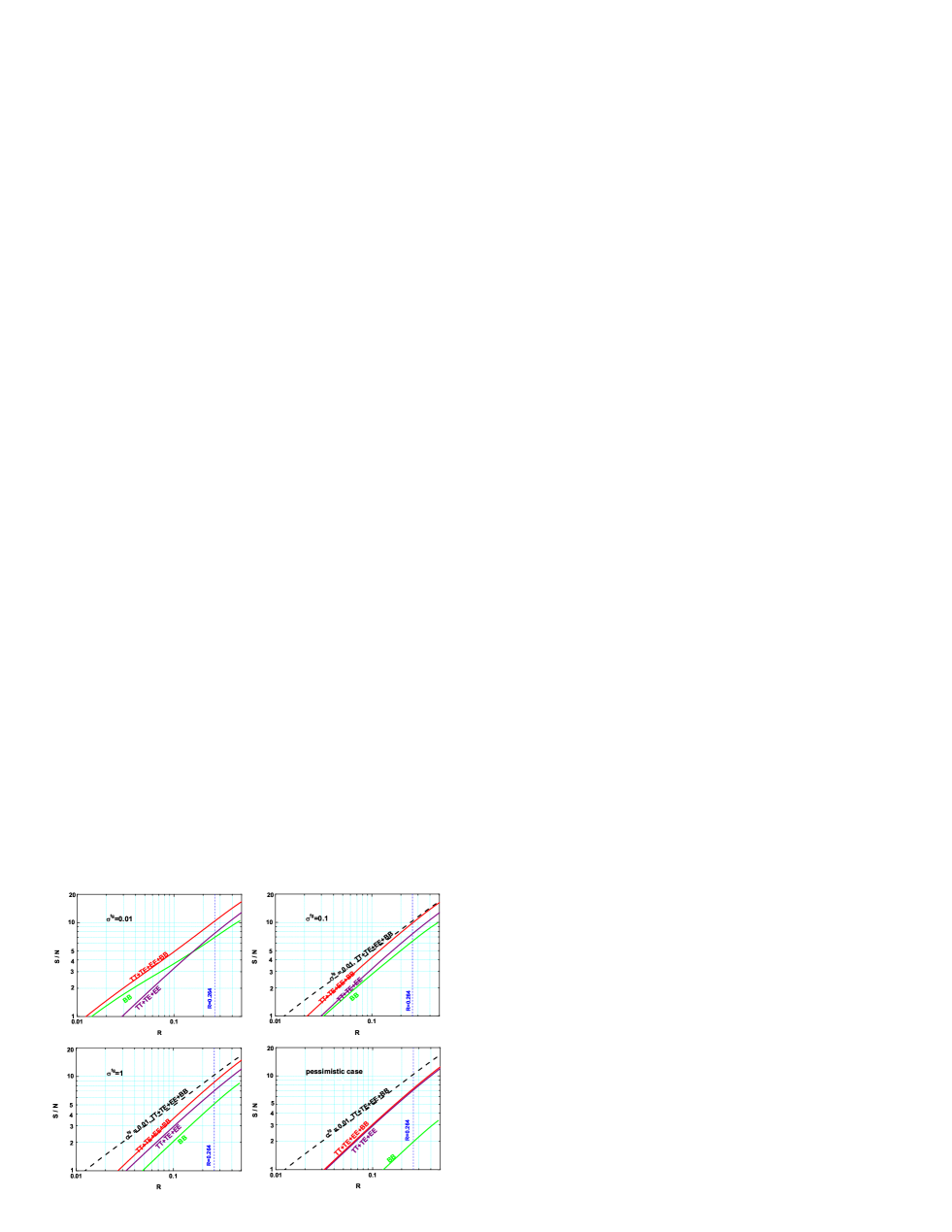
Figure 8: The decomposition of the total $S/N$ into contributions from different information channels. Four panels describe different assumptions about foreground cleaning and noises. The $S/N$ line from the upper left panel for the optimistic case $\sigma^{\rm fg}=0.01$ is copied as a broken line in other panels.

In Fig. 9 we illustrate the decomposition of the total $S/N$ into contributions from individual multipoles $\ell$:

$$(S/N)^{2}=\sum_{\ell}(S/N)_{\ell}^{2}.$$ (30)

We show the contributing terms $(S/N)_{\ell}^{2}$ for three combinations of information channels, $TT+TE+EE+BB$, $TT+TE+EE$ and $BB$ alone, and for two opposite extreme assumptions about foreground cleaning and noises, namely, $\sigma^{\rm fg}=0.01$ and the pessimistic case. The calculations are done for the benchmark model (16) with $R=0.264$. Surely, the total $S/N$ exhibited in the upper left and lower right panels of Fig. 8 is recovered with the help of Eq.(30) from the sum of the terms $(S/N)_{\ell}^{2}$ shown in the left and right panels of Fig. 9, respectively.

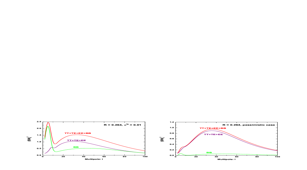
Figure 9: The individual terms $(S/N)_{\ell}^{2}$ as functions of $\ell$ for various combinations of information channels and two opposite assumptions about residual foreground contamination and noises. The calculations are done for the ML model (16) with $R=0.264$.

It is seen from the left panel of Fig. 9 that in the case of deep cleaning the $BB$ channel is particularly sensitive to the very low multipoles $\ell\simeq 10$ associated with the reionization era. At the same time, the right panel of Fig. 9 demonstrates that in the pessimistic case most of $S/N$ comes from $TT+TE+EE$ combination and, specifically, from the interval of mutlipoles $\ell\sim(20-60)$ associated with the recombination era.

Finally, we want to discuss possible improvements in our forecasts. They will be achievable, if 7 frequency channels, instead of 3, can be used for data analysis, and/or if the less restrictive Dust B model, instead of the Dust A model, turns out to be correct, and/or if 28 months of observations, instead of 14 months, can be reached. In Fig. 10 we show the results for the scenario where 7 frequency channels are used and the Dust B model is correct. Similarly to Fig. 7, the left panel shows $S/N$ calculated assuming that only $R$ is being determined from the data, whereas the right panel shows a more realistic case in which all perturbation parameters are unknown. In the later case, the $S/N$ for the ML model (16) with $R=0.264$ increases up to the level $S/N=5.56$ as compared with $S/N=4.04$ that we found in the right panel of Fig. 7 for 3 frequency channels and the Dust A model.

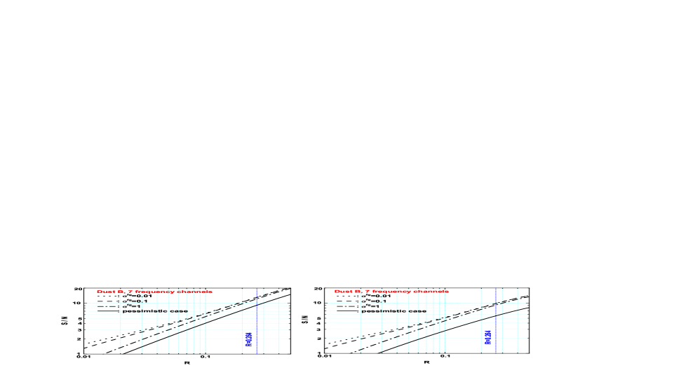
Figure 10: The improved signal-to-noise ratio $S/N$ for the scenario where the Dust B model is correct and the instrumental noises are smaller because of the 7 frequency channels used, instead of 3, in data analysis. The left panel shows $S/N$ with $\Delta R=1/\sqrt{F_{RR}}$, while the right panel shows $S/N$ with $\Delta R=\sqrt{(F^{-1})_{RR}}$.

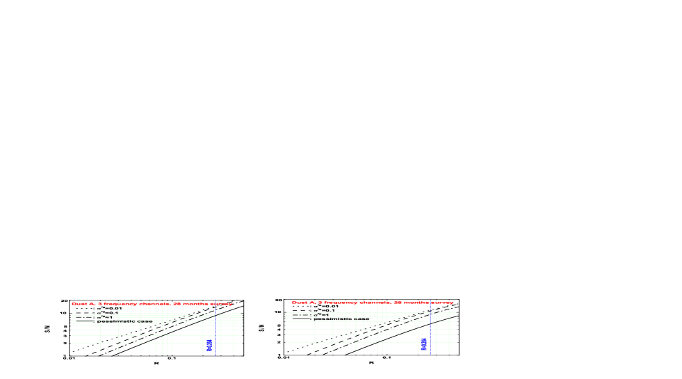
Figure 11: The improved $S/N$ for 28 months of observations. Other assumptions are the same as in Fig. 7.

The two panels in Fig. 11 illustrate the improvements, as compared with the two panels in Fig. 7, arising from the longer, 28-month, survey instead of the nominal 14 months survey. The $S/N$ for the benchmark model $R=0.264$ increases up to $S/N=5.39$ even in the pessimistic case, right panel. The decomposition of $S/N$ appearing in the left panel of Fig. 11 into contributions from different information channels is presented in Fig. 12. One can see that the relative role of the $BB$ channel has increased. (The prospects of $B$-mode detection in the conditions of low instrumental and foreground noises have been analyzed in EG .)

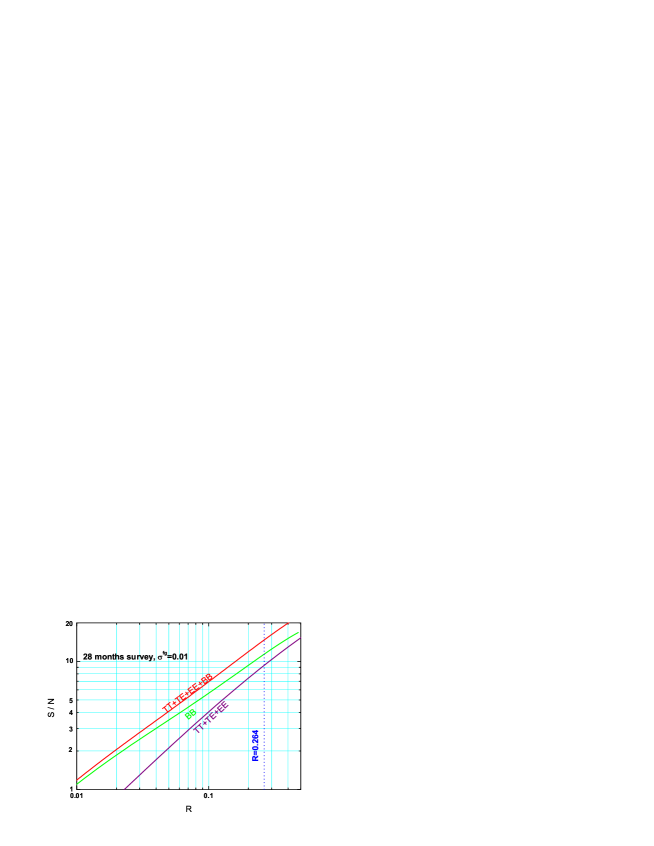
Figure 12: Decomposition of the total $S/N$ figuring in the left panel of Fig. 11 into contributions from different information channels. In the assumed conditions of deep cleaning $\sigma^{\rm fg}=0.01$, the $BB$ alone is more informative than the combination $TT+TE+EE$.

VI Theoretical frameworks that will be accepted or rejected by Planck observations

Our forecast for the Planck mission, as any forecast in nature, can prove its value only after actual observation. We predict sunny days of confident detection of relic gravitational waves, but the reality can turn out to be gloomy days of continuing uncertainty. One can illustrate this point with the help of probability distributions in Fig. 4. We expect that Planck observations will continue the trend of exhibiting narrower likelihoods with maximum in the area near the WMAP7 ML value $R=0.264$. Then the detailed analysis in Sec. V explains the reasons for our optimism. But, in principle, the reality can happen to be totally different. From the position of pure logic it is still possible that the Planck data, although making the new likelihood curve much narrower, will also shift the maximum of this curve to the point $R=0$. In this case, instead of confident detection we will have to speak about “tight upper limits”. We do not think, though, that this is going to happen. What kind of conclusions about theoretical models can we make if the likelihood curve comes out as we anticipated?

As was already mentioned in Sec. II, the theory of quantum-mechanical generation of cosmological perturbations implies a reasonable guess for the true value of $R$: $R\in[0.01,1]$. We shall call it a model $M_{1}$. At the same time, the most advanced string-inspired inflationary theories predict $R$ somewhere in the interval $R\in[0,10^{-24}]$. We shall call it a model $M_{2}$. The inflationary calculations can be perfectly alright in their stringy part, but the observational predictions are entirely hanging on the inflationary “classic result”, and therefore should fall together with it, on purely theoretical grounds. But this is not the point of our present discussion. We wish to conduct a Bayesian comparison of models $M_{1}$ and $M_{2}$, regardless of the motivations that stayed behind these models.

The model $M_{1}$ suggests that the quadrupole ratio $R$ should lie in the range $[0.01,1]$ with a uniform prior in this range: $P_{\rm prior}(R|M_{1})=c_{1}$ for $R\in[0.01,1]$. The model $M_{2}$ suggests that $R$ should lie in the range $[0,10^{-24}]$ with a uniform prior in this range: $P_{\rm prior}(R|M_{2})=c_{2}$ for $R\in[0,10^{-24}]$. The constants $c_{1}$ and $c_{2}$ are determined from normalization of the prior distributions, $c_{1}=(0.99)^{-1}$ and $c_{2}=10^{24}$. The predicted interval of possible values of $R$ is much wider for $M_{1}$ than for $M_{2}$. Therefore, $M_{1}$ is penalized by a much smaller normalization constant $c_{1}$ than $c_{2}$. The observed data allow one to compare the two models quantitatively with the help of the Bayes factor $K_{12}$ bayes

$$K_{12}\equiv\frac{\int_{0}^{\infty}P_{\rm prior}(R|M_{1})\mathcal{L}(R)dR}{\int_{0}^{\infty}P_{\rm prior}(R|M_{2})\mathcal{L}(R)dR},$$ (31)

where $\mathcal{L}$ is the likelihood function of $R$ derived from the observation.

We shall start from the existing WMAP7 data. The likelihood function as a function of $R$ is shown by a red solid line in Fig. 4. Calculating the Bayes factor according to Eq.(31) we find $K_{12}=1.61$, i.e. $\ln K_{12}=0.48$. As expected, this value of the Bayes factor, although indicative, does not provide sufficient reason for the rejection of model $M_{2}$ in favor of $M_{1}$.

With more accurate Planck observations the situation will change dramatically, if the WMAP7 maximum likelihood set of parameters (16) is correct. To make calculation in Eq.(31), we adopt a Gaussian shape of the likelihood function $\mathcal{L}$ with maximum at $R=0.264$ and $R\geq 0$. The standard deviation is taken as $\Delta R=0.065$. This value follows from the analysis of $S/N$ for Planck mission and corresponds to the derived $S/N=4.04$ in the pessimistic case. Then the calculation of $K_{12}$ gives the value $K_{12}=579.23$, i.e. $\ln K_{12}=6.36$. In accordance with Jeffrey’s interpretation bayes , this result shows that the Planck observations will decisively reject the model $M_{2}$ in favor of $M_{1}$.

If Planck observations are as accurate as expected, and if our assumptions about Planck’s likelihood function are correct, the models much less extreme than $M_{2}$ will also be decisively rejected. We introduce the model $M_{3}$ with a flat prior in the range $R\in[0,x]$ and ask the question for which $x$ the Bayes factor $K_{13}$ exceeds the critical value $K_{13}=100$ ($\ln K_{13}=4.61$) bayes which is required for decisive exclusion of the model. The calculation gives $x=0.05$. This means that under the conditions listed above the Planck experiment will be able to decisively reject any theoretical framework that predicts $R<0.05$. In terms of the parameter $r$ this means the exclusion of all models with $r<0.095$.

VII Conclusions

The analysis of the WMAP7 data release amplifies observational indications in favor of relic gravitational waves in the Universe. The WMAP3, WMAP5, and WMAP7 temperature and polarization data in the interval of multipoles $2\leq\ell\leq 100$ persistently point out to one and the same area in the space of perturbation parameters. It includes a considerable amount of gravitational waves expressed in terms of the parameter $R=0.264$, and somewhat blue primordial spectra with indices $n_{s}=1.111$ and $n_{t}=0.111$. If the maximum likelihood set of parameters that we derived from this analysis is a fair representation of the reality, the relic gravitational waves will be detected more confidently by Planck observations. Even under pessimistic assumption about hindering factors, the expected signal-to-noise ratio should be at the level $S/N=4.04$.

Acknowledgements We acknowledge the use of the LAMBDA and CAMB Websites. W. Z. is partially supported by Chinese NSF Grants No. 10703005, and No. 10775119 and the Foundation for University Excellent Young Teacher by the Ministry of Zhejiang Education.

References

- (1) E. Komatsu et al., arXiv: 1001.4538.
- (2) D. Larson et al., arXiv: 1001.4635.
- (3) W. Zhao, D. Baskaran and L. P. Grishchuk, Phys. Rev. D 80, 083005 (2009).
- (4) Planck Collaboration, The Science Programme of Planck [astro-ph/0604069].
- (5) D. Baskaran, L. P. Grishchuk and W. Zhao, In Proceedings of MG12 meeting (World Scientific, Singapore, to be published) [arXiv:1004.0804].
- (6) Ya. B. Zeldovich, Pis’ma Zh. Eksp. Teor. Fiz. 7, 579 (1981); L. P. Grishchuk and Ya. B. Zeldovich, in Quantum Structure of Space and Time, Eds. M. Duff and C. Isham, (Cambridge University Press, Cambridge, 1982), p. 409; Ya. B. Zeldovich, ‘Cosmological field theory for observational astronomers’, Sov. Sci. Rev. E Astrophys. Space Phys. Vol. 5, pp. 1-37 (1986) (http://nedwww.ipac.caltech.edu/level5/Zeldovich/Zel_contents.html); A. Vilenkin, in The Future of Theoretical Physics and Cosmology, Eds. G. W. Gibbons, E. P. S. Shellard and S. J. Rankin (Cambridge University Press, Cambridge, England, 2003).
- (7) L. P. Grishchuk, Space Science Reviews 148, 315 (2009) [arXiv:0903.4395].
- (8) L. P. Grishchuk, Zh. Eksp. Teor. Fiz. 67, 825 (1974) [Sov. Phys. JETP 40, 409 (1975)]; Ann. N. Y. Acad. Sci 302, 439 (1977); Pis’ma Zh. Eksp. Teor. Fiz. 23, 326 (1976) [JETP Lett. 23, 293 (1976)]; Usp. Fiz. Nauk 121, 629 (1977) [Sov. Phys. Usp. 20, 319 (1977)].
- (9) L. P. Grishchuk, ‘Discovering Relic Gravitational Waves in Cosmic Microwave Background Radiation’, chapter in General Relativity and John Archibald Wheeler, Eds. I. Ciufolini and R. Matzner (Springer, New York, 2010, pp.151-199) [arXiv:0707.3319].
- (10) L. P. Grishchuk and M. Solokhin, Phys. Rev. D 43, 2566 (1991).
- (11) A. Lewis, A. Challinor and A. Lasenby, Astrophys. J. 538, 473 (2000); http://camb.info/.
- (12) W. Zhao, D. Baskaran and L. P. Grishchuk, Phys. Rev. D 79, 023002 (2009).
- (13) W. Zhao and D. Baskaran, Phys. Rev. D 79, 083003 (2009); W. Zhao and W. Zhang, Phys. Lett. B 677, 16 (2009).
- (14) R. K. Sachs and A. M. Wolfe, Astrophys. J. 147, 73 (1967); L. P. Grishchuk and Ya. B. Zel’dovich, Soviet Astronomy 22, 125 (1978); V. A. Rubakov, M. V. Sazhin, A. V. Veryaskin, Phys. Lett. B 115, 189 (1982); A. Polnarev, Sov. Astron. 29, 607 (1985); A. A. Starobinskii, Pis’ma Astron. Zh. 11, 323 (1985); D. Harari and M. Zaldarriaga, Phys. Lett. B 319, 96 (1993); L. P. Grishchuk, Phys. Rev. Lett. 70, 2371 (1993). R. Crittenden, J. R. Bond, R. L. Davis, G. Efstathiou and P. J. Steinhardt, Phys. Rev. Lett. 71, 324 (1993); R. A. Frewin, A. G. Polnarev and P. Coles, Mon. Not. R. Astron. Soc. 266, L21 (1994).
- (15) M. Zaldarriaga and U. Seljak, Phys. Rev. D 55, 1830 (1997); M. Kamionkowski, A. Kosowsky and A. Stebbins, Phys. Rev. D 55, 7368 (1997).
- (16) J. R. Pritchard and M. Kamionkowski, Ann. Phys. (N.Y.) 318, 2 (2005); W. Zhao and Y. Zhang, Phys. Rev. D 74, 083006 (2006); T. Y. Xia and Y. Zhang, Phys. Rev. D 78, 123005 (2008).
- (17) D. Baskaran, L. P. Grishchuk and A. G. Polnarev, Phys. Rev. D 74, 083008 (2006).
- (18) B. G. Keating, A. G. Polnarev, N. J. Miller and D. Baskaran, Int. J. Mod. Phys. A 21, 2459 (2006); R. Flauger and S. Weinberg, Phys. Rev. D 75, 123505 (2007); Y. Zhang, W. Zhao, X. Z. Er, H. X. Miao and T. Y. Xia, Int. J. Mod. Phys. D 17, 1105 (2008).
- (19) M. S. Turner and M. White, Phys. Rev. D 53, 6822 (1996); S. Chongchitnan and G. Efstathiou, Phys. Rev. D 73, 083511 (2006).
- (20) http://lambda.gsfc.nasa.gov/.
- (21) A. Gelman, J. B. Carlin, H. S. Stern and D. B. Rubin, Bayesian Data Analysis (ACRC Press Company, Boca Raton, USA, 2004); W. R. Gilks, S. Richardson and D. J. Spiegelhalter, Markov Chain Monte Carlo in Practice (ACRC Press Company, Boca Raton, USA, 1996).
- (22) A. Lewis and S. Bridle, Phys. Rev. D 66, 103511 (2002).
- (23) E. Komatsu et al., Astrophys. J. Suppl. Ser. 180, 330 (2009).
- (24) G. Efstathiou and S. Gratton, J. Cosmol. Astropart. Phys. 06, 011 (2009).
- (25) H. Jeffreys, Theory of Probability (Oxford University Press, Oxford, 1961).