RIP-Based Near-Oracle Performance Guarantees for Subspace-Pursuit, CoSaMP, and Iterative Hard-Thresholding

Abstract

This paper presents an average case denoising performance analysis for the Subspace Pursuit (SP), the CoSaMP and the IHT algorithms. This analysis considers the recovery of a noisy signal, with the assumptions that (i) it is corrupted by an additive random white Gaussian noise; and (ii) it has a $K$-sparse representation with respect to a known dictionary ${\bf D}$. The proposed analysis is based on the Restricted-Isometry-Property (RIP), establishing a near-oracle performance guarantee for each of these algorithms. The results for the three algorithms differ in the bounds’ constants and in the cardinality requirement (the upper bound on $K$ for which the claim is true).

Similar RIP-based analysis was carried out previously for the Dantzig Selector (DS) and the Basis Pursuit (BP). Past work also considered a mutual-coherence-based analysis of the denoising performance of the DS, BP, the Orthogonal Matching Pursuit (OMP) and the thresholding algorithms. This work differs from the above as it addresses a different set of algorithms. Also, despite the fact that SP, CoSaMP, and IHT are greedy-like methods, the performance guarantees developed in this work resemble those obtained for the relaxation-based methods (DS and BP), suggesting that the performance is independent of the sparse representation entries contrast and magnitude.

I Introduction

I-A General – Pursuit Methods for Denoising

The area of sparse approximation (and compressed sensing as one prominent manifestation of its applicability) is an emerging field that get much attention in the last decade. In one of the most basic problems posed in this field, we consider a noisy measurement vector ${\bf y}\in\mathbb{R}^{m}$ of the form

$${\bf y}={\bf D}{\bf x}+{\bf e},$$ (I.1)

where ${\bf x}\in\mathbb{R}^{N}$ is the signal’s representation with respect to the dictionary ${\bf D}\in\mathbb{R}^{m\times N}$ where $N\geq m$. The vector ${\bf e}\in\mathbb{R}^{m}$ is an additive noise, which is assumed to be an adversial disturbance, or a random vector – e.g., white Gaussian noise with zero mean and variance $\sigma^{2}$. We further assume that the columns of ${\bf D}$ are normalized, and that the representation vector ${\bf x}$ is $K$-sparse, or nearly so. Our goal is to find the $K$-sparse vector ${\bf x}$ that approximates the measured signal ${\bf y}$. Put formally, this reads

$$\min_{{\bf x}}~{}\left\|{\bf y}-{\bf D}{\bf x}\right\|_{2}~{}~{}\text{ subject to }\left\|{\bf x}\right\|_{0}=K,$$ (I.2)

where $\left\|{\bf x}\right\|_{0}$ is the $\ell_{0}$ pseudo-norm that counts the number of non-zeros in the vector ${\bf x}$. This problem is quite hard and problematic [1, 2, 3, 4]. A straight forward search for the solution of (I.2) is an NP hard problem as it requires a combinatorial search over the support of ${\bf x}$ [5]. For this reason, approximation algorithms were proposed – these are often referred to as pursuit algorithms.

One popular pursuit approach is based on $\ell_{1}$ relaxation and known as the Basis Pursuit (BP) [6] or the Lasso [7]. The BP aims at minimizing the relaxed objective

$$(P1): \min_{{\bf x}}\left\|{\bf x}\right\|_{1}\text{ subject to }\left\|{\bf y}-{\bf D}{\bf x}\right\|_{2}^{2}\leq\epsilon_{\bf BP}^{2},$$ (I.3)

where $\epsilon_{\bf BP}$ is a constant related to the noise power. This minimizing problem has an equivalent form:

$$(BP): \min_{{\bf x}} \frac{1}{2}\left\|{\bf y}-{\bf D}{\bf x}\right\|_{2}^{2}+\gamma_{BP}\left\|{\bf x}\right\|_{1},$$ (I.4)

where $\gamma_{BP}$ is a constant related to $\epsilon_{\bf BP}$. Another $\ell_{1}$-based relaxed algorithm is the Dantzig Selector (DS), as proposed in [8]. The DS aims at minimizing

$$(DS):\min_{{\bf x}}\left\|{\bf x}\right\|_{1}\text{ subject to }\left\|{\bf D}^{*}({\bf y}-{\bf D}{\bf x})\right\|_{\infty}\leq\epsilon_{\bf DS},$$ (I.5)

where $\epsilon_{\bf DS}$ is a constant related to the noise power.

A different pursuit approach towards the approximation of the solution of (I.2) is the greedy strategy [9, 10, 11], leading to algorithms such as the Matching Pursuit (MP) and the Orthogonal Matching Pursuit (OMP). These algorithms build the solution ${\bf x}$ one non-zero entry at a time, while greedily aiming to reduce the residual error $\left\|{\bf y}-{\bf D}{\bf x}\right\|_{2}^{2}$.

The last family of pursuit methods we mention here are greedy-like algorithms that differ from MP and OMP in two important ways: (i) Rather than accumulating the desired solution one element at a time, a group of non-zeros is identified together; and (ii) As opposed to the MP and OMP, these algorithms enable removal of elements from the detected support. Algorithms belonging to this group are the Regularized OMP (ROMP) [12], the Compressive Sampling Matching Pursuit (CoSaMP) [13], the Subspace-Pursuit (SP) [14], and the Iterative Hard Thresholding (IHT) [15]. This paper focuses on this specific family of methods, as it poses an interesting compromise between the simplicity of the greedy methods and the strong abilities of the relaxed algorithms.

I-B Performance Analysis – Basic Tools

Recall that we aim at recovering the (deterministic!) sparse representation vector ${\bf x}$. We measure the quality of the approximate solution $\hat{{\bf x}}$ by the Mean-Squared-Error (MSE)

$$\operatorname{MSE}(\hat{{\bf x}})=E\left\|{\bf x}-\hat{{\bf x}}\right\|_{2}^{2},$$ (I.6)

where the expectation is taken over the distribution of the noise. Therefore, our goal is to get as small as possible error. The question is, how small can this noise be? In order to answer this question, we first define two features that characterize the dictionary ${\bf D}$ – the mutual coherence and the Restricted Isometry Property (RIP). Both are used extensively in formulating the performance guarantees of the sort developed in this paper.

The mutual-coherence $\mu$ [16, 17, 18] of a matrix ${\bf D}$ is the largest absolute normalized inner product between different columns from ${\bf D}$. The larger it is, the more problematic the dictionary is, because in such a case we get that columns in ${\bf D}$ are too much alike.

Turning to the RIP, it is said that ${\bf D}$ satisfies the $K$-RIP condition with parameter $\delta_{K}$ if it is the smallest value that satisfies

$$(1-\delta_{K})\left\|{\bf x}\right\|_{2}^{2}\leq\left\|{\bf D}{\bf x}\right\|_{2}^{2}\leq(1+\delta_{K})\left\|{\bf x}\right\|_{2}^{2}$$ (I.7)

for any $K$-sparse vector ${\bf x}$ [19, 20].

These two measures are related by $\delta_{K}\leq(K-1)\mu$ [21]. The RIP is a stronger descriptor of ${\bf D}$ as it characterizes groups of $K$ columns from ${\bf D}$, whereas the mutual coherence “sees” only pairs. On the other hand, computing $\mu$ is easy, while the evaluation of $\delta_{K}$ is prohibitive in most cases. An exception to this are random matrices ${\bf D}$ for which the RIP constant is known (with high probability). For example, if the entries of $\sqrt{m}{\bf D}$ are drawn from a white Gaussian distribution and $m\geq CK\log(N/K)/\epsilon^{2}$, then with a very high probability $\delta_{K}\leq\epsilon$ [19, 22].

We return now to the question we posed above: how small can the error $\operatorname{MSE}(\hat{{\bf x}})$ be? Consider an oracle estimator that knows the support of ${\bf x}$, i.e. the locations of the $K$ non-zeros in this vector. The oracle estimator obtained as a direct solution of the problem posed in (I.2) is easily given by

$$\hat{{\bf x}}_{oracle}={\bf D}_{T}^{\dagger}{\bf y},$$ (I.8)

where $T$ is the support of ${\bf x}$ and ${\bf D}_{T}$ is a sub-matrix of ${\bf D}$ that contains only the columns involved in the support $T$. Its MSE is given by [8]

$$\operatorname{MSE}(\hat{{\bf x}}_{oracle})=E\left\|{\bf x}-\hat{{\bf x}}_{oracle}\right\|_{2}^{2}=E\left\|{\bf D}_{T}^{\dagger}{\bf e}\right\|_{2}^{2}.$$ (I.9)

In the case of a random noise, as described above, this error becomes

$$\operatorname{MSE}(\hat{{\bf x}}_{oracle}) = E\left\|{\bf D}_{T}^{\dagger}{\bf e}\right\|_{2}^{2}$$

$$= \operatorname{trace}\left\{({\bf D}^{*}_{T}{\bf D}_{T})^{-1}\right\}\sigma^{2}$$

$$\leq \frac{K}{1-\delta_{K}}\sigma^{2}.$$

This is the smallest possible error, and it is proportional to the number of non-zeros $K$ multiplied by $\sigma^{2}$. It is natural to ask how close do we get to this best error by practical pursuit methods that do not assume the knowledge of the support. This brings us to the next sub-section.

I-C Performance Analysis – Known Results

There are various attempts to bound the MSE of pursuit algorithms. Early works considered the adversary case, where the noise can admit any form as long as its norm is bounded [23, 24, 2, 1]. These works gave bounds on the reconstruction error in the form of a constant factor ($Const>1$) multiplying the noise power,

$$\left\|{\bf x}-\hat{{\bf x}}\right\|^{2}_{2}\leq Const\cdot\left\|{\bf e}\right\|_{2}^{2}.$$ (I.11)

Notice that the cardinality of the representation plays no role in this bound, and all the noise energy is manifested in the final error.

One such example is the work by Candès and Tao, reported in [20], which analyzed the BP error. This work have shown that if the dictionary ${\bf D}$ satisfies $\delta_{K}+\delta_{2K}+\delta_{3K}<1$ then the BP MSE is bounded by a constant times the energy of the noise, as shown above. The condition on the RIP was improved to $\delta_{2K}<\sqrt{2}-1$ in [25]. Similar tighter bounds are $\delta_{1.625K}<\sqrt{2}-1$ and $\delta_{3K}<4-2\sqrt{3}$ [26], or $\delta_{K}<0.307$ [27]. The advantage of using the RIP in the way described above is that it gives a uniform guarantee: it is related only to the dictionary and sparsity level.

Next in line to be analyzed are the greedy methods (MP, OMP, Thr) [23, 1]. Unlike the BP, these algorithms where shown to be more sensitive, incapable of providing a uniform guarantee for the reconstruction. Rather, beyond the dependence on the properties of ${\bf D}$ and the sparsity level, the guarantees obtained depend also on the ratio between the noise power and the absolute values of the signal representation entries.

Interestingly, the greedy-like approach, as practiced in the ROMP, the CoSaMP, the SP, and the IHT algorithms, was found to be closer is spirit to the BP, all leading to uniform guarantees on the bounded MSE. The ROMP was the first of these algorithms to be analyzed [12], leading to the more strict requirement $\delta_{2K}<0.03/\sqrt{\log K}$. The CoSaMP [13] and the SP [14] that came later have similar RIP conditions without the $\log K$ factor, where the SP result is slightly better. The IHT algorithm was also shown to have a uniform guarantee for bounded error of the same flavor as shown above [15].

All the results mentioned above deal with an adversial noise, and therefore give bounds that are related only to the noise power with a coefficient that is larger than $1$, implying that no effective denoising is to be expected. This is natural since we consider the worst case results, where the noise can be concentrated in the places of the non-zero elements of the sparse vector. To obtain better results, one must change the perspective and consider a random noise drawn from a certain distribution.

The first to realize this and exploit this alternative point of view were Candes and Tao in the work reported in [8] that analyzed the DS algorithm. As mentioned above, the noise was assumed to be random zero-mean white Gaussian noise with a known variance $\sigma^{2}$. For the choice $\epsilon_{DS}=\sqrt{2(1+a)\log{N}}\cdot\sigma$, and requiring $\delta_{2K}+\delta_{3K}<1$, the minimizer of (I.5), $\hat{{\bf x}}_{DS}$, was shown to obey

$$\left\|{\bf x}-\hat{{\bf x}}_{DS}\right\|^{2}_{2}\leq C_{DS}^{2}\cdot(2(1+a)\log N)\cdot K\sigma^{2},$$ (I.12)

with probability exceeding $1-(\sqrt{\pi(1+a)\log N}\cdot N^{a})^{-1}$, where $C_{DS}=4/(1-2\delta_{3K})$. Up to a constant and a $\log N$ factor, this bound is the same as the oracle’s one in (I.9). The $\log N$ factor in (I.12) in unavoidable, as proven in [28], and therefore this bound is optimal up to a constant factor.

A similar result was presented in [29] for the BP, showing that the solution of (I.4) for the choice $\gamma_{BP}=\sqrt{8\sigma^{2}(1+a)\log N}$, and requiring $\delta_{2K}+3\delta_{3K}<1$, satisfies

$$\left\|{\bf x}-\hat{{\bf x}}_{DS}\right\|^{2}_{2}\leq C_{BP}^{2}\cdot(2(1+a)\log N)\cdot K\sigma^{2}$$ (I.13)

with probability exceeding $1-(N^{a})^{-1}$. This result is weaker than the one obtained for the DS in three ways: (i) It gives a smaller probability of success; (ii) The constant $C_{BP}$ is larger, as shown in [21] ($C_{BP}\geq 32/\kappa^{4}$, where $\kappa<1$ is defined in [29]); and (iii) The condition on the RIP is stronger.

Mutual-Coherence based results for the DS and BP were derived in [30, 21]. In [21] results were developed also for greedy algorithms – the OMP and the thresholding. These results rely on the contrast and magnitude of the entries of ${\bf x}$. Denoting by $\hat{{\bf x}}_{greedy}$ the reconstruction result of the thresholding and the OMP, we have

$$\left\|{\bf x}-\hat{{\bf x}}_{greedy}\right\|^{2}_{2}\leq C_{greedy}^{2}\cdot(2(1+a)\log N)\cdot K\sigma^{2},$$ (I.14)

where $C_{greedy}\leq 2$ and with probability exceeds $1-(\sqrt{\pi(1+a)\log N}\cdot N^{a})^{-1}$. This result is true for the OMP and thresholding under the condition

$$\frac{\left|{\bf x}_{min}\right|-2\sigma\sqrt{2(1+a)\log N}}{(2K-1)\mu}\geq\left\{\begin{array}[]{cc}\left|{\bf x}_{min}\right|&\text{OMP}\\ |{\bf x}_{max}|&\text{THR}\end{array}\right.,$$ (I.17)

where $|{\bf x}_{min}|$ and $|{\bf x}_{max}|$ are the minimal and maximal non-zero absolute entries in ${\bf x}$.

I-D This Paper Contribution

We have seen that greedy algorithms’ success is dependent on the magnitude of the entries of ${\bf x}$ and the noise power, which is not the case for the DS and BP. It seems that there is a need for pursuit algorithms that, on one hand, will enjoy the simplicity and ease of implementation as in the greedy methods, while being guaranteed to perform as well as the BP and DS. Could the greedy-like methods (ROMP, CoSaMP, SP, IHT) serve this purpose? The answer was shown to be positive for the adversial noise assumption, but these results are too weak, as they do not show the true denoising effect that such algorithm may lead to. In this work we show that the answer remains positive for the random noise assumption.

More specifically, in this paper we present RIP-based near-oracle performance guarantees for the SP, CoSaMP and IHT algorithms (in this order). We show that these algorithms get uniform guarantees, just as for the relaxation based methods (the DS and BP). We present the analysis that leads to these results and we provide explicit values for the constants in the obtained bounds.

The organization of this paper is as follows: In Section II we introduce the notation and propositions used for our analysis. In Section III we develop RIP-based bounds for the SP, CoSaMP and the IHT algorithms for the adversial case. Then we show how we can derive from these a new set of guarantees for near oracle performance that consider the noise as random. We develop fully the steps for the SP, and outline the steps needed to get the results for the CoSaMP and IHT. In Section IV we present some experiments that show the performance of the three methods, and a comparison between the theoretical bounds and the empirical performance. In Section V we consider the nearly-sparse case, extending all the above results. Section VI concludes our work.

II Notation and Preliminaries

The following notations are used in this paper:

• $\operatorname{supp}({\bf x})$ is the support of ${\bf x}$ (a set with the locations of the non-zero elements of ${\bf x}$).

• $\left|\operatorname{supp}({\bf x})\right|$ is the size of the set $\operatorname{supp}({\bf x})$.

• $\operatorname{supp}({\bf x},K)$ is the support of the largest $K$ magnitude elements in ${\bf x}$.

• ${\bf D}_{T}$ is a matrix composed of the columns of the matrix ${\bf D}$ of the set $T$.

• In a similar way, ${\bf x}_{T}$ is a vector composed of the entries of the vector ${\bf x}$ over the set $T$.

• $T^{C}$ symbolizes the complementary set of $T$.

• $T-\tilde{T}$ is the set of all the elements contained in $T$ but not in $\tilde{T}$.

• We will denote by $T$ the set of the non-zero places of the original signal ${\bf x}$; As such, $\left|T\right|\leq K$ when ${\bf x}$ is $K$-sparse.

• ${\bf x}_{K}$ is the vector with the $K$ dominant elements of ${\bf x}$.

• The projection of a vector ${\bf y}$ to the subspace spanned by the columns of the matrix ${\bf A}$ (assumed to have more rows than columns) is denoted by $\operatorname{proj}({\bf y},{\bf A})={\bf A}{\bf A}^{\dagger}{\bf y}$. The residual is $\operatorname{resid}({\bf y},{\bf A})={\bf y}-{\bf A}{\bf A}^{\dagger}{\bf y}$.

• $T_{e}$ is the subset of columns of size $K$ in ${\bf D}$ that gives the maximum correlation with the noise vector ${\bf e}$, namely,

  $$T_{e}=\operatornamewithlimits{argmax}_{T\left|~{}|T|=K\right.}\left\|{\bf D}_{T}^{*}{\bf e}\right\|_{2}$$ (II.1)

• $T_{{\bf e},p}$ is a generalization of $T_{{\bf e}}$ where $T$ in (II.1) is of size $pK$, $p\in\mathbb{N}$. It is clear that $\left\|{\bf D}_{T_{{\bf e},p}}^{*}{\bf e}\right\|_{2}\leq p\left\|{\bf D}_{T_{{\bf e}}}^{*}{\bf e}\right\|_{2}$.

The proofs in this paper use several propositions from [13, 14]. We bring these in this Section, so as to keep the discussion complete.

Proposition II.1

[Proposition 3.1 in [13]] Suppose ${\bf D}$ has a restricted isometry constant $\delta_{K}$. Let $T$ be a set of $K$ indices or fewer. Then

$$\left\|{\bf D}_{T}^{*}{\bf y}\right\|_{2}\leq\sqrt{1+\delta_{K}}\left\|{\bf y}\right\|_{2}$$

$$\left\|{\bf D}_{T}^{\dagger}{\bf y}\right\|_{2}\leq\frac{1}{\sqrt{1-\delta_{K}}}\left\|{\bf y}\right\|_{2}$$

$$\left\|{\bf D}_{T}^{*}{\bf D}_{T}{\bf x}\right\|_{2}\lesseqqgtr(1\pm\delta_{K})\left\|{\bf x}\right\|_{2}$$

$$\left\|({\bf D}_{T}^{*}{\bf D}_{T})^{-1}{\bf x}\right\|_{2}\lesseqqgtr\frac{1}{1\pm\delta_{K}}\left\|{\bf x}\right\|_{2}$$

where the last two statements contain upper and lower bounds, depending on the sign chosen.

Proposition II.2

[Lemma 1 in [14]] Consequences of the RIP:

1. (Monotonicity of $\delta_{K}$) For any two integers $K\leq K^{\prime}$, $\delta_{K}\leq\delta_{K^{\prime}}$.

2. (Near-orthogonality of columns) Let $I,J\subset\{1,...,N\}$ be two disjoint sets ($I\cap J=\emptyset$). Suppose that $\delta_{\left|I\right|+\left|J\right|}<1$. For arbitrary vectors ${\bf a}\in\mathbb{R}^{\left|I\right|}$ and ${\bf b}\in\mathbb{R}^{\left|J\right|}$,

   $$\left|\langle{\bf D}_{I}{\bf a},{\bf D}_{J}{\bf b}\rangle\right|\leq\delta_{\left|I\right|+\left|J\right|}\left\|{\bf a}\right\|_{2}\left\|{\bf b}\right\|_{2}$$

   and

   $$\left\|{\bf D}_{I}^{*}{\bf D}_{J}{\bf b}\right\|_{2}\leq\delta_{\left|I\right|+\left|J\right|}\left\|{\bf b}\right\|_{2}.$$

Proposition II.3

[Lemma 2 in [14]] Projection and Residue:

1. (Orthogonality of the residue) For an arbitrary vector ${\bf y}\in\mathbb{R}^{m}$ and a sub-matrix ${\bf D}_{I}\in\mathbb{R}^{m\times K}$ of full column-rank, let ${\bf y}_{r}=\operatorname{resid}({\bf y,{\bf D}_{I}})$. Then ${\bf D}^{*}_{I}{\bf y}_{r}=0$.

2. (Approximation of the projection residue) Consider a matrix ${\bf D}\in\mathbb{R}^{m\times N}$. Let $I,J\subset\{1,...,N\}$ be two disjoint sets, $I\cap J=\emptyset$, and suppose that $\delta_{\left|I\right|+\left|J\right|}<1$. Let ${\bf y}\in\operatorname{span}({\bf D}_{I})$, ${\bf y}_{p}=\operatorname{proj}({\bf y},{\bf D}_{J})$ and ${\bf y}_{r}=\operatorname{resid}({\bf y},{\bf D}_{J})$. Then

   $$\left\|{\bf y}_{p}\right\|_{2}\leq\frac{\delta_{\left|I\right|+\left|J\right|}}{1-\delta_{\max(\left|I\right|,\left|J\right|)}}\left\|{\bf y}\right\|_{2}$$

   and

   $$\left(1-\frac{\delta_{\left|I\right|+\left|J\right|}}{1-\delta_{\max(\left|I\right|,\left|J\right|)}}\right)\left\|{\bf y}\right\|_{2}\leq\left\|{\bf y}_{r}\right\|_{2}\leq\left\|{\bf y}\right\|_{2}.$$

Proposition II.4

[Corollary 3.3 in [13]] Suppose that ${\bf D}$ has an RIP constant $\delta_{\tilde{K}}$. Let $T_{1}$ be an arbitrary set of indices, and let ${\bf x}$ be a vector. Provided that $\tilde{K}\geq\left|T_{1}\cup\operatorname{supp}({\bf x})\right|$, we obtain that

$$\left\|{\bf D}^{*}_{T_{1}}{\bf D}_{T^{C}_{1}}{\bf x}_{T^{C}_{1}}\right\|_{2}\leq\delta_{\tilde{K}}\left\|{\bf x}_{T^{C}_{1}}\right\|_{2}.$$ (II.2)

III Near oracle performance of the algorithms

Our goal in this section is to find error bounds for the SP, CoSaMP and IHT reconstructions given the measurement from (I.1). We will first find bounds for the case where ${\bf e}$ is an adversial noise using the same techniques used in [14, 13]. In these works and in [15], the reconstruction error was bounded by a constant times the noise power in the same form as in (I.11). In this work, we will derive a bound that is a constant times $\left\|{\bf D}_{T_{\bf e}}^{*}{\bf e}\right\|_{2}$ (where $T_{\bf e}$ is as defined in the previous section). Armed with this bound, we will change perspective and look at the case where ${\bf e}$ is a white Gaussian noise, and derive a near-oracle performance result of the same form as in (I.12), using the same tools used in [8].

III-A Near oracle performance of the SP algorithm

We begin with the SP pursuit method, as described in Algorithm 1. SP holds a temporal solution with $K$ non-zero entries, and in each iteration it adds an additional set of $K$ candidate non-zeros that are most correlated with the residual, and prunes this list back to $K$ elements by choosing the dominant ones. We use a constant number of iterations as a stopping criterion but different stopping criteria can be sought, as presented in [14].

Algorithm 1 Subspace Pursuit Algorithm [Algorithm 1 in [14]]

0:  $K,{\bf D},{\bf y}$ where ${\bf y}={\bf D}{\bf x}+{\bf e}$, $K$ is the cardinality of ${\bf x}$ and ${\bf e}$ is the additive noise.

0:  $\hat{{\bf x}}_{SP}$: $K$-sparse approximation of ${\bf x}$

  Initialize the support: $T^{0}=\emptyset$.

  Initialize the residual: ${\bf y}_{r}^{0}={\bf y}$.

  while halting criterion is not satisfied do

     Find new support elements: $T_{\Delta}=\operatorname{supp}({\bf D}^{*}{\bf y}^{\ell-1}_{r},K)$.

     Update the support: $\tilde{T}^{\ell}=T^{\ell-1}\cup T_{\Delta}$.

     Compute the representation: ${\bf x}_{p}={\bf D}^{{\dagger}}_{\tilde{T}^{\ell}}{\bf y}$.

     Prune small entries in the representation: $T^{\ell}=\operatorname{supp}({\bf x}_{p},K)$.

     Update the residual: ${\bf y}_{r}^{\ell}=\operatorname{resid}({\bf y},{\bf D}_{T^{\ell}})$.

  end while

  Form the final solution: $\hat{{\bf x}}_{SP,(T^{\ell})^{C}}=0$ and $\hat{{\bf x}}_{SP,T^{\ell}}={\bf D}^{{\dagger}}_{T^{\ell}}{\bf y}$.

Theorem III.1

The SP solution at the $\ell$-th iteration satisfies the recurrence inequality

$$\left\|{\bf x}_{T-T^{\ell}}\right\|_{2} \leq \frac{2\delta_{3K}(1+\delta_{3K})}{(1-\delta_{3K})^{3}}\left\|{\bf x}_{T-T^{\ell-1}}\right\|_{2}$$

$$+\frac{6-6\delta_{3K}+4\delta_{3K}^{2}}{(1-\delta_{3K})^{3}}\left\|{\bf D}_{T_{\bf e}}^{*}{\bf e}\right\|_{2}.$$

For $\delta_{3K}\leq 0.139$ this leads to

$$\left\|{\bf x}_{T-T^{\ell}}\right\|_{2}\leq 0.5\left\|{\bf x}_{T-T^{\ell-1}}\right\|_{2}+8.22\left\|{\bf D}_{T_{\bf e}}^{*}{\bf e}\right\|_{2}.$$ (III.2)

Proof: The proof of the inequality in (III.1) is given in Appendix A. Note that the recursive formula given (III.1) has two coefficients, both functions of $\delta_{3K}$. Fig. 1 shows these coefficients as a function of $\delta_{3K}$. As can be seen, under the condition $\delta_{3K}\leq 0.139$, it holds that the coefficient multiplying $\left\|{\bf x}_{T-T^{\ell-1}}\right\|_{2}$ is lesser or equal to $0.5$, while the coefficient multiplying $\left\|{\bf D}_{T_{\bf e}}^{*}{\bf e}\right\|_{2}$ is lesser or equal to $8.22$, which completes our proof. $\Box$

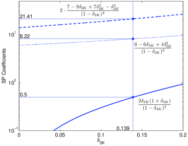
Figure 1: The coefficients in (III.1) and (III.5) as functions of $\delta_{3K}$.

Corollary III.2

Under the condition $\delta_{3K}\leq 0.139$, the SP algorithm satisfies

$$\left\|{\bf x}_{T-T^{\ell}}\right\|_{2}\leq 2^{-\ell}\left\|{\bf x}\right\|_{2}+2\cdot 8.22\left\|{\bf D}_{T_{\bf e}}^{*}{\bf e}\right\|_{2}.$$ (III.3)

In addition, After at most

$$\ell^{*}=\left\lceil\log_{2}\left(\frac{\left\|{\bf x}\right\|_{2}}{\left\|{\bf D}_{T_{\bf e}}^{*}{\bf e}\right\|_{2}}\right)\right\rceil$$ (III.4)

iterations, the solution $\hat{{\bf x}}_{SP}$ leads to an accuracy

$$\left\|{\bf x}-\hat{{\bf x}}_{SP}\right\|_{2}\leq C_{SP}\left\|{\bf D}_{T_{\bf e}}^{*}{\bf e}\right\|_{2},$$ (III.5)

where

$$C_{SP}=2\cdot\frac{7-9\delta_{3K}+7\delta_{3K}^{2}-\delta_{3K}^{3}}{(1-\delta_{3K})^{4}}\leq 21.41$$ (III.6)

Proof: Starting with (III.2), and applying it recursively we obtain

$$\left\|{\bf x}_{T-T^{\ell}}\right\|_{2}\leq 0.5\left\|{\bf x}_{T-T^{\ell-1}}\right\|_{2}+8.22\left\|{\bf D}_{T_{\bf e}}^{*}{\bf e}\right\|_{2}$$ (III.7)

$$~{}~{}~{}~{}~{}\leq 0.5^{2}\left\|{\bf x}_{T-T^{\ell-2}}\right\|_{2}+8.22\cdot(0.5+1)\left\|{\bf D}_{T_{\bf e}}^{*}{\bf e}\right\|_{2}$$

$$~{}~{}~{}~{}~{}\leq\ldots$$

$$~{}~{}~{}~{}~{}\leq 0.5^{k}\left\|{\bf x}_{T-T^{\ell-k}}\right\|_{2}+8.22\cdot\left(\sum_{j=0}^{k-1}0.5^{j}\right)\left\|{\bf D}_{T_{\bf e}}^{*}{\bf e}\right\|_{2}.$$

Setting $k=\ell$ leads easily to (III.3), since $\left\|{\bf x}_{T-T^{0}}\right\|_{2}=\left\|{\bf x}_{T}\right\|_{2}=\left\|{\bf x}\right\|_{2}$.

Plugging the number of iterations $\ell^{*}$ as in (III.4) to (III.3) yields

$$\left\|{\bf x}_{T-T^{\ell^{*}}}\right\|_{2}$$ (III.8)

$$~{}~{}~{}~{}~{}\leq 2^{-\ell^{*}}\left\|{\bf x}\right\|_{2}+2\cdot\frac{6-6\delta_{3K}+4\delta_{3K}^{2}}{(1-\delta_{3K})^{3}}\left\|{\bf D}_{T_{\bf e}}^{*}{\bf e}\right\|_{2}$$

$$~{}~{}~{}~{}~{}\leq\left(1+2\cdot\frac{6-6\delta_{3K}+4\delta_{3K}^{2}}{(1-\delta_{3K})^{3}}\right)\left\|{\bf D}_{T_{\bf e}}^{*}{\bf e}\right\|_{2}.$$

We define $\hat{T}\triangleq T^{\ell^{*}}$ and bound the reconstruction error $\left\|{\bf x}-\hat{{\bf x}}_{SP}\right\|_{2}$. First, notice that $\left\|{\bf x}\right\|=\left\|{\bf x}_{\hat{T}}\right\|+\left\|{\bf x}_{T-\hat{T}}\right\|$, simply because the true support $T$ can be divided into $\hat{T}$ and the complementary part, $T-\hat{T}$. Using the facts that $\hat{{\bf x}}_{SP}={\bf D}^{\dagger}_{\hat{T}}{\bf y}$, ${\bf y}={\bf D}_{T}{\bf x}_{T}+{\bf e}$, and the triangle inequality, we get

$$\left\|{\bf x}-\hat{{\bf x}}_{SP}\right\|_{2}$$ (III.9)

$$~{}~{}~{}~{}~{}\leq\left\|{\bf x}_{\hat{T}}-{\bf D}^{\dagger}_{\hat{T}}{\bf y}\right\|_{2}+\left\|{\bf x}_{T-\hat{T}}\right\|_{2}$$

$$~{}~{}~{}~{}~{}=\left\|{\bf x}_{\hat{T}}-{\bf D}^{\dagger}_{\hat{T}}({\bf D}_{T}{\bf x}_{T}+{\bf e})\right\|_{2}+\left\|{\bf x}_{T-\hat{T}}\right\|_{2}$$

$$~{}~{}~{}~{}~{}\leq\left\|{\bf x}_{\hat{T}}-{\bf D}^{\dagger}_{\hat{T}}{\bf D}_{T}{\bf x}_{T}\right\|_{2}+\left\|{\bf D}^{\dagger}_{\hat{T}}{\bf e}\right\|_{2}+\left\|{\bf x}_{T-\hat{T}}\right\|_{2}.$$

We proceed by breaking the term ${\bf D}_{T}{\bf x}_{T}$ into the sum ${\bf D}_{T\cap\hat{T}}{\bf x}_{T\cap\hat{T}}+{\bf D}_{T-\hat{T}}{\bf x}_{T-\hat{T}}$, and obtain

$$\left\|{\bf x}-\hat{{\bf x}}_{SP}\right\|_{2} \leq \left\|{\bf x}_{\hat{T}}-{\bf D}^{\dagger}_{\hat{T}}{\bf D}_{T\cap\hat{T}}{\bf x}_{T\cap\hat{T}}\right\|_{2}$$

$$+\left\|{\bf D}^{\dagger}_{\hat{T}}{\bf D}_{T-\hat{T}}{\bf x}_{T-\hat{T}}\right\|_{2}+\left\|({\bf D}^{*}_{\hat{T}}{\bf D}_{\hat{T}})^{-1}{\bf D}^{*}_{\hat{T}}{\bf e}\right\|_{2}+\left\|{\bf x}_{T-\hat{T}}\right\|_{2}.$$

The first term in the above inequality vanishes, since ${\bf D}_{T\cap\hat{T}}{\bf x}_{T\cap\hat{T}}={\bf D}_{\hat{T}}{\bf x}_{\hat{T}}$ (recall that ${\bf x}_{\hat{T}}$ outside the support $T$ has zero entries that do not contribute to the multiplication). Thus, we get that ${\bf x}_{\hat{T}}-{\bf D}^{\dagger}_{\hat{T}}{\bf D}_{T\cap\hat{T}}{\bf x}_{T\cap\hat{T}}={\bf x}_{\hat{T}}-{\bf D}^{\dagger}_{\hat{T}}{\bf D}_{\hat{T}}{\bf x}_{\hat{T}}=0$. The second term can be bounded using Propositions II.1 and II.2,

$$\left\|{\bf D}^{\dagger}_{\hat{T}}{\bf D}_{T-\hat{T}}{\bf x}_{T-\hat{T}}\right\|_{2}=\left\|({\bf D}^{*}_{\hat{T}}{\bf D}_{\hat{T}})^{-1}{\bf D}^{*}_{\hat{T}}{\bf D}_{T-\hat{T}}{\bf x}_{T-\hat{T}}\right\|_{2}$$

$$~{}~{}~{}~{}~{}\leq\frac{1}{1-\delta_{K}}\left\|{\bf D}^{*}_{\hat{T}}{\bf D}_{T-\hat{T}}{\bf x}_{T-\hat{T}}\right\|_{2}\leq\frac{\delta_{2K}}{1-\delta_{K}}\left\|{\bf x}_{T-\hat{T}}\right\|_{2}.$$

Similarly, the third term is bounded using Propositions II.1, and we obtain

$$\left\|{\bf x}-\hat{{\bf x}}_{SP}\right\|_{2} \leq \left(1+\frac{\delta_{2K}}{1-\delta_{K}}\right)\left\|{\bf x}_{T-\hat{T}}\right\|_{2}+\frac{1}{1-\delta_{K}}\left\|{\bf D}^{*}_{\hat{T}}{\bf e}\right\|_{2}$$

$$\leq \frac{1}{1-\delta_{3K}}\left\|{\bf x}_{T-\hat{T}}\right\|_{2}+\frac{1}{1-\delta_{3K}}\left\|{\bf D}^{*}_{\hat{T}}{\bf e}\right\|_{2},$$

where we have replaced $\delta_{K}$ and $\delta_{2K}$ with $\delta_{3K}$, thereby bounding the existing expression from above. Plugging (III.8) into this inequality leads to

$$\left\|{\bf x}-\hat{{\bf x}}_{SP}\right\|_{2} \leq \frac{1}{1-\delta_{3K}}\left(2+2\cdot\frac{6-6\delta_{3K}+4\delta_{3K}^{2}}{(1-\delta_{3K})^{3}}\right)\left\|{\bf D}^{*}_{\hat{T}}{\bf e}\right\|_{2}$$

$$= 2\cdot\frac{7-9\delta_{3K}+7\delta_{3K}^{2}-\delta_{3K}^{3}}{(1-\delta_{3K})^{4}}\left\|{\bf D}^{*}_{\hat{T}}{\bf e}\right\|_{2}.$$

Applying the condition $\delta_{3K}\leq 0.139$ on this equation leads to the result in (III.5). $\Box$

For practical use we may suggest a simpler term for $\ell^{*}$. Since $\left\|{\bf D}_{T_{\bf e}}^{*}{\bf e}\right\|_{2}$ is defined by the subset that gives the maximal correlation with the noise, and it appears in the denominator of $\ell^{*}$, it can be replaced with the average correlation, thus $\ell^{*}\approx\left\lceil\log_{2}\left(\left\|{\bf x}\right\|_{2}/\sqrt{K}\sigma\right)\right\rceil$.

Now that we have a bound for the SP algorithm for the adversial case, we proceed and consider a bound for the random noise case, which will lead to a near-oracle performance guarantee for the SP algorithm.

Theorem III.3

Assume that ${\bf e}$ is a white Gaussian noise vector with variance $\sigma^{2}$ and that the columns of ${\bf D}$ are normalized. If the condition $\delta_{3K}\leq 0.139$ holds, then with probability exceeding $1-(\sqrt{\pi(1+a)\log{N}}\cdot N^{a})^{-1}$ we obtain

$$\left\|{\bf x}-\hat{{\bf x}}_{SP}\right\|_{2}^{2}\leq C_{SP}^{2}\cdot(2(1+a)\log{N})\cdot K\sigma^{2}.$$ (III.11)

Proof: Following Section 3 in [8] it holds true that ${\bf P}\left(\sup_{i}\left|{\bf D}_{i}^{*}{\bf e}\right|>\sigma\cdot\sqrt{2(1+a)\log{N}}\right)\leq 1-(\sqrt{\pi(1+a)\log{N}}\cdot N^{a})^{-1}.$ Combining this with (III.5), and bearing in mind that $|T_{e}|=K$, we get the stated result. $\Box$

As can be seen, this result is similar to the one posed in [8] for the Dantzig-Selector, but with a different constant – the one corresponding to DS is $\approx 5.5$ for the RIP requirement used for the SP. For both algorithms, smaller values of $\delta_{3K}$ provide smaller constants.

III-B Near oracle performance of the CoSaMP algorithm

We continue with the CoSaMP pursuit method, as described in Algorithm 2. CoSaMP, in a similar way to the SP, holds a temporal solution with $K$ non-zero entries, with the difference that in each iteration it adds an additional set of $2K$ (instead of $K$) candidate non-zeros that are most correlated with the residual. Anther difference is that after the punning step in SP we use a matrix inversion in order to calculate a new projection for the $K$ dominant elements, while in the CoSaMP we just take the biggest $K$ elements. Here also, we use a constant number of iterations as a stopping criterion while different stopping criteria can be sought, as presented in [13].

Algorithm 2 CoSaMP Algorithm [Algorithm 2.1 in [13]]

0:  $K,{\bf D},{\bf y}$ where ${\bf y}={\bf D}{\bf x}+{\bf e}$, $K$ is the cardinality of ${\bf x}$ and ${\bf e}$ is the additive noise.

0:  $\hat{{\bf x}}_{CoSaMP}$: $K$-sparse approximation of ${\bf x}$

  Initialize the support: $T^{0}=\emptyset$.

  Initialize the residual: ${\bf y}_{r}^{0}={\bf y}$.

  while halting criterion is not satisfied do

     Find new support elements: $T_{\Delta}=\operatorname{supp}({\bf D}^{*}{\bf y}^{\ell-1}_{r},2K)$.

     Update the support: $\tilde{T^{\ell}}=T^{\ell-1}\cup T_{\Delta}$.

     Compute the representation: ${\bf x}_{p}={\bf D}^{{\dagger}}_{\tilde{T}^{\ell}}{\bf y}$.

     Prune small entries in the representation: $T^{\ell}=\operatorname{supp}({\bf x}_{p},K)$.

     Update the residual: ${\bf y}_{r}^{\ell}={\bf y}-{\bf D}_{T^{\ell}}({\bf x}_{p})_{T^{\ell}}$.

  end while

  Form the final solution: $\hat{{\bf x}}_{CoSaMP,(T^{\ell})^{C}}=0$ and $\hat{{\bf x}}_{CoSaMP,T^{\ell}}=({\bf x}_{p})_{T^{\ell}}$.

In the analysis of the CoSaMP that comes next, we follow the same steps as for the SP to derive a near-oracle performance guarantee. Since the proofs are very similar to those of the SP, and those found in [13], we omit most of the derivations and present only the differences.

Theorem III.4

The CoSaMP solution at the $\ell$-th iteration satisfies the recurrence inequality

$$\left\|{\bf x}-\hat{{\bf x}}_{CoSaMP}^{\ell}\right\|_{2} \leq \frac{4\delta_{4K}}{(1-\delta_{4K})^{2}}\left\|{\bf x}-\hat{{\bf x}}_{CoSaMP}^{\ell-1}\right\|_{2}$$

$$+\frac{14-6\delta_{4K}}{(1-\delta_{4K})^{2}}\left\|{\bf D}_{T_{{\bf e}}}^{*}{\bf e}\right\|_{2}$$

For $\delta_{4K}\leq 0.1$ this leads to

$$\left\|{\bf x}-\hat{{\bf x}}_{CoSaMP}^{\ell}\right\|_{2}\leq 0.5\left\|{\bf x}-\hat{{\bf x}}_{CoSaMP}^{\ell-1}\right\|_{2}+16.6\left\|{\bf D}_{T_{\bf e}}^{*}{\bf e}\right\|_{2}.$$ (III.13)

Proof: The proof of the inequality in (III.4) is given in Appendix D. In a similar way to the proof in the SP case, under the condition $\delta_{4K}\leq 0.1$, it holds that the coefficient multiplying $\left\|{\bf x}-\hat{{\bf x}}_{CoSaMP}^{\ell-1}\right\|_{2}$ is smaller or equal to $0.5$, while the coefficient multiplying $\left\|{\bf D}_{T_{\bf e}}^{*}{\bf e}\right\|_{2}$ is smaller or equal to $16.6$, which completes our proof. $\Box$

Corollary III.5

Under the condition $\delta_{4K}\leq 0.1$, the CoSaMP algorithm satisfies

$$\left\|{\bf x}-\hat{{\bf x}}_{CoSaMP}^{\ell}\right\|_{2}\leq 2^{-\ell}\left\|{\bf x}\right\|_{2}+2\cdot 16.6\left\|{\bf D}_{T_{\bf e}}^{*}{\bf e}\right\|_{2}.$$ (III.14)

In addition, After at most

$$\ell^{*}=\left\lceil\log_{2}\left(\frac{\left\|{\bf x}\right\|_{2}}{\left\|{\bf D}_{T_{\bf e}}^{*}{\bf e}\right\|_{2}}\right)\right\rceil$$ (III.15)

iterations, the solution $\hat{{\bf x}}_{CoSaMP}$ leads to an accuracy

$$\left\|{\bf x}-\hat{{\bf x}}_{CoSaMP}^{\ell}\right\|_{2}\leq C_{CoSaMP}\left\|{\bf D}_{T_{\bf e}}^{*}{\bf e}\right\|_{2},$$ (III.16)

where

$$C_{CoSaMP}=\frac{29-14\delta_{4K}+\delta_{4K}^{2}}{(1-\delta_{4K})^{2}}\leq 34.1.$$ (III.17)

Proof: Starting with (III.13), and applying it recursively, in the same way as was done in the proof of Corollary III.5, we obtain

$$\left\|{\bf x}-\hat{{\bf x}}_{CoSaMP}^{\ell}\right\|_{2} \leq 0.5^{k}\left\|{\bf x}-\hat{{\bf x}}_{CoSaMP}^{\ell-k}\right\|_{2}$$

$$+16.6\cdot\left(\sum_{j=0}^{k-1}0.5^{j}\right)\left\|{\bf D}_{T_{\bf e}}^{*}{\bf e}\right\|_{2}.$$

Setting $k=\ell$ leads easily to (III.14), since $\left\|{\bf x}-\hat{{\bf x}}_{CoSaMP}^{0}\right\|_{2}=\left\|{\bf x}\right\|_{2}$.

Plugging the number of iterations $\ell^{*}$ as in (III.15) to (III.14) yields

$$\left\|{\bf x}-\hat{{\bf x}}_{CoSaMP}^{\ell}\right\|_{2} \leq 2^{-\ell^{*}}\left\|{\bf x}\right\|_{2}+2\cdot\frac{14-6\delta_{4K}}{(1-\delta_{4K})^{2}}\left\|{\bf D}_{T_{\bf e}}^{*}{\bf e}\right\|_{2}$$

$$\leq \left(1+2\cdot\frac{14-6\delta_{4K}}{(1-\delta_{4K})^{2}}\right)\left\|{\bf D}_{T_{\bf e}}^{*}{\bf e}\right\|_{2}$$

$$\leq \frac{29-14\delta_{4K}+\delta_{4K}^{2}}{(1-\delta_{4K})^{2}}\left\|{\bf D}_{T_{\bf e}}^{*}{\bf e}\right\|_{2}.$$

Applying the condition $\delta_{4K}\leq 0.1$ on this equation leads to the result in (III.16). $\Box$

As for the SP, we move now to the random noise case, which leads to a near-oracle performance guarantee for the CoSaMP algorithm.

Theorem III.6

Assume that ${\bf e}$ is a white Gaussian noise vector with variance $\sigma^{2}$ and that the columns of ${\bf D}$ are normalized. If the condition $\delta_{4K}\leq 0.1$ holds, then with probability exceeding $1-(\sqrt{\pi(1+a)\log{N}}\cdot N^{a})^{-1}$ we obtain

$$\left\|{\bf x}-\hat{{\bf x}}_{CoSaMP}\right\|_{2}^{2}\leq C_{CoSaMP}^{2}\cdot(2(1+a)\log{N})\cdot K\sigma^{2}.$$ (III.19)

Proof: The proof is identical to the one of Theorem III.6. $\Box$

Fig. 2 shows a graph of $C_{CoSaMP}$ as a function of $\delta_{4K}$. In order to compare the CoSaMP to SP, we also introduce in this figure a graph of $C_{SP}$ versus $\delta_{4K}$ (replacing $\delta_{3K}$). Since $\delta_{3K}\leq\delta_{4K}$, the constant $C_{SP}$ is actually better than the values shown in the graph, and yet, it can be seen that even in this case we get $C_{SP}<C_{CoSaMP}$. In addition, the requirement for the SP is expressed with respect to $\delta_{3K}$, while the requirement for the CoSaMP is stronger and uses $\delta_{4K}$.

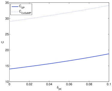
Figure 2: The constants of the SP and CoSaMP algorithms as a funtion of $\delta_{4K}$

With comparison to the results presented in [21] for the OMP and the thresholding, the results obtained for the CoSaMP and SP are uniform, expressed only with respect to the properties of the dictionary ${\bf D}$. These algorithms’ validity is not dependent on the values of the input vector ${\bf x}$, its energy, or the noise power. The condition used is the RIP, which implies constraints only on the used dictionary and the sparsity level.

III-C Near oracle performance of the IHT algorithm

The IHT algorithm, presented in Algorithm 3, uses a different strategy than the SP and the CoSaMP. It applies only multiplications by ${\bf D}$ and ${\bf D}^{*}$, and a hard thresholding operator. In each iteration it calculates a new representation and keeps its $K$ largest elements. As for the SP and CoSaMP, here as well we employ a fixed number of iterations as a stopping criterion.

Algorithm 3 IHT Algorithm [Equation 7 in [15]]

0:  $K,{\bf D},{\bf y}$ where ${\bf y}={\bf D}{\bf x}+{\bf e}$, $K$ is the cardinality of ${\bf x}$ and ${\bf e}$ is the additive noise.

0:  $\hat{{\bf x}}_{IHT}$: $K$-sparse approximation of ${\bf x}$

  Initialize the support: $T^{0}=\emptyset$.

  Initialize the representation: ${\bf x}^{0}_{IHT}=0$.

  while halting criterion is not satisfied do

     Compute the representation: ${\bf x}_{p}=\hat{{\bf x}}_{IHT}^{\ell-1}+{\bf D}^{*}({\bf y}-{\bf D}\hat{{\bf x}}_{IHT}^{\ell-1})$.

     Prune small entries in the representation: $T^{\ell}=\operatorname{supp}({\bf x}_{p},K)$.

     Update the representation: $\hat{{\bf x}}_{IHT,(T^{\ell})^{C}}^{\ell}=0$ and $\hat{{\bf x}}_{IHT,T^{\ell}}^{\ell}=({\bf x}_{p})_{T^{\ell}}$.

  end while

  Form the final solution: $\hat{{\bf x}}_{IHT,(T^{\ell})^{C}}=0$ and $\hat{{\bf x}}_{IHT,T^{\ell}}=({\bf x}_{p})_{T^{\ell}}$.

Similar results, as of the SP and CoSaMP methods, can be sought for the IHT method. Again, the proofs are very similar to the ones shown before for the SP and the CoSaMP and thus only the differences will presented.

Theorem III.7

The IHT solution at the $\ell$-th iteration satisfies the recurrence inequality

$$\left\|{\bf x}-\hat{{\bf x}}^{\ell}_{IHT}\right\|_{2}\leq\sqrt{8}\delta_{3K}\left\|{\bf x}-\hat{{\bf x}}_{IHT}^{\ell-1}\right\|_{2}+4\left\|{\bf D}^{*}_{T_{{\bf e}}}{\bf e}\right\|_{2}.$$ (III.20)

For $\delta_{3K}\leq\frac{1}{\sqrt{32}}$ this leads to

$$\left\|{\bf x}-\hat{{\bf x}}^{\ell}_{IHT}\right\|_{2}\leq 0.5\left\|{\bf x}-\hat{{\bf x}}_{IHT}^{\ell-1}\right\|_{2}+4\left\|{\bf D}^{*}_{T_{{\bf e}}}{\bf e}\right\|_{2}.$$ (III.21)

Proof: Our proof is based on the proof of Theorem 5 in [15], and only major modifications in the proof will be presented here. Using the definition ${\bf r}^{\ell}\triangleq{\bf x}-\hat{{\bf x}}_{IHT}^{\ell}$, and an inequality taken from Equation (22) in [15], it holds that

$$\left\|{\bf x}-\hat{{\bf x}}^{\ell}_{IHT}\right\|_{2}\leq 2\left\|{\bf x}_{T\cup T^{\ell}}-({\bf x}_{p})_{T\cup T^{\ell}}\right\|_{2}$$ (III.22)

$$~{}~{}~{}~{}=2\left\|{\bf x}_{T\cup T^{\ell}}-\hat{{\bf x}}^{\ell-1}_{T\cup T^{\ell}}-{\bf D}^{*}_{T\cup T^{\ell}}{\bf D}{\bf r}^{\ell-1}-{\bf D}^{*}_{T\cup T^{\ell}}{\bf e}\right\|_{2}$$

$$~{}~{}~{}~{}=2\left\|{\bf r}_{T\cup T^{\ell}}^{\ell-1}-{\bf D}^{*}_{T\cup T^{\ell}}{\bf D}{\bf r}^{\ell-1}-{\bf D}^{*}_{T\cup T^{\ell}}{\bf e}\right\|_{2},$$

where the equality emerges from the definition ${\bf x}_{p}=\hat{{\bf x}}_{IHT}^{\ell-1}+{\bf D}^{*}({\bf y}-{\bf D}\hat{{\bf x}}_{IHT}^{\ell-1})=\hat{{\bf x}}_{IHT}^{\ell-1}+{\bf D}^{*}({\bf D}{\bf x}+{\bf e}-{\bf D}\hat{{\bf x}}_{IHT}^{\ell-1}).$

The support of ${\bf r}^{\ell-1}$ is over $T\cup T^{\ell-1}$ and thus it is also over $T\cup T^{\ell}\cup T^{\ell-1}$. Based on this, we can divide ${\bf D}{\bf r}^{\ell-1}$ into a part supported on $T^{\ell-1}-T^{\ell}\cup T$ and a second part supported on $T^{\ell}\cup T$. Using this and the triangle inequality with (III.22), we obtain

$$\left\|{\bf x}-\hat{{\bf x}}^{\ell}_{IHT}\right\|_{2}$$ (III.23)

$$~{}~{}\leq 2\left\|{\bf r}^{\ell-1}_{T\cup T^{\ell}}-{\bf D}^{*}_{T\cup T^{\ell}}{\bf D}{\bf r}^{\ell-1}\right\|_{2}+2\left\|{\bf D}^{*}_{T\cup T^{\ell}}{\bf e}\right\|_{2}$$

$$~{}~{}=2\left\|({\bf I}-{\bf D}^{*}_{T\cup T^{\ell}}{\bf D}_{T\cup T^{\ell}}){\bf r}^{\ell-1}_{T\cup T^{\ell}}\right.$$

$$~{}~{}~{}~{}\left.-{\bf D}^{*}_{T\cup T^{\ell}}{\bf D}_{T^{\ell-1}-T\cup T^{\ell}}{\bf r}^{\ell-1}_{T^{\ell-1}-T\cup T^{\ell}}\right\|_{2}+2\left\|{\bf D}^{*}_{T\cup T^{\ell}}{\bf e}\right\|_{2}$$

$$~{}~{}\leq 2\left\|({\bf I}-{\bf D}^{*}_{T\cup T^{\ell}}{\bf D}_{T\cup T^{\ell}}){\bf r}^{\ell-1}_{T\cup T^{\ell}}\right\|_{2}$$

$$~{}~{}~{}~{}+2\left\|{\bf D}^{*}_{T\cup T^{\ell}}{\bf D}_{T^{\ell-1}-T\cup T^{\ell}}{\bf r}^{\ell-1}_{T^{\ell-1}-T\cup T^{\ell}}\right\|_{2}+2\left\|{\bf D}^{*}_{T_{{\bf e}},2}{\bf e}\right\|_{2}$$

$$~{}~{}\leq 2\delta_{2K}\left\|{\bf r}^{\ell-1}_{T\cup T^{\ell}}\right\|_{2}+2\delta_{3K}\left\|{\bf r}^{\ell-1}_{T^{\ell-1}-T\cup T^{\ell}}\right\|_{2}+4\left\|{\bf D}^{*}_{T_{{\bf e}}}{\bf e}\right\|_{2}.$$

The last inequality holds because the eigenvalues of $({\bf I}-{\bf D}^{*}_{T\cup T^{\ell}}{\bf D}_{T\cup T^{\ell}})$ are in the range $[-\delta_{2K},\delta_{2K}]$, the size of the set $T\cup T^{\ell}$ is smaller than $2K$, the sets $T\cup T^{\ell}$ and $T^{\ell-1}-T\cup T^{\ell}$ are disjoint, and of total size of these together is equal or smaller than $3K$. Note that we have used the definition of $T_{{\bf e},2}$ as given in Section II.

We proceed by observing that $\left\|{\bf r}^{\ell-1}_{T^{\ell-1}-T\cup T^{\ell}}\right\|_{2}+\left\|{\bf r}^{\ell-1}_{T\cup T^{\ell}}\right\|_{2}\leq\sqrt{2}\left\|{\bf r}^{\ell-1}\right\|_{2}$, since these vectors are orthogonal. Using the fact that $\delta_{2K}\leq\delta_{3K}$ we get (III.20) from (III.23). Finally, under the condition $\delta_{3K}\leq 1/\sqrt{32}$, it holds that the coefficient multiplying $\left\|{\bf x}-\hat{{\bf x}}_{IHT}^{\ell-1}\right\|_{2}$ is smaller or equal to $0.5$, which completes our proof. $\Box$

Corollary III.8

Under the condition $\delta_{3K}\leq 1/\sqrt{32}$, the IHT algorithm satisfies

$$\left\|{\bf x}-\hat{{\bf x}}_{IHT}^{\ell}\right\|_{2}\leq 2^{-\ell}\left\|{\bf x}\right\|_{2}+8\left\|{\bf D}_{T_{\bf e}}^{*}{\bf e}\right\|_{2}.$$ (III.24)

In addition, After at most

$$\ell^{*}=\left\lceil\log_{2}\left(\frac{\left\|{\bf x}\right\|_{2}}{\left\|{\bf D}_{T_{\bf e}}^{*}{\bf e}\right\|_{2}}\right)\right\rceil$$ (III.25)

iterations, the solution $\hat{{\bf x}}_{IHT}$ leads to an accuracy

$$\left\|{\bf x}-\hat{{\bf x}}_{IHT}^{\ell}\right\|_{2}\leq C_{IHT}\left\|{\bf D}_{T_{\bf e}}^{*}{\bf e}\right\|_{2},$$ (III.26)

where

$$C_{IHT}=9.$$ (III.27)

Proof: The proof is obtained following the same steps as in Corollaries III.2 and III.5. $\Box$

Finally, considering a random noise instead of an adversial one, we get a near-oracle performance guarantee for the IHT algorithm, as was achieved for the SP and CoSaMP.

Theorem III.9

Assume that ${\bf e}$ is a white Gaussian noise with variance $\sigma^{2}$ and that the columns of ${\bf D}$ are normalized. If the condition $\delta_{3K}\leq 1/\sqrt{32}$ holds, then with probability exceeding $1-(\sqrt{\pi(1+a)\log{N}}\cdot N^{a})^{-1}$ we obtain

$$\left\|{\bf x}-\hat{{\bf x}}_{IHT}\right\|_{2}^{2}\leq C_{IHT}^{2}\cdot(2(1+a)\log{N})\cdot K\sigma^{2}.$$ (III.28)

Proof: The proof is identical to the one of Theorem III.6. $\Box$

A comparison between the constants achieved by the IHT, SP and DS is presented in Fig. 3. The CoSaMP constant was omitted since it is bigger than the one of the SP and it is dependent on $\delta_{4K}$ instead of $\delta_{3K}$. The figure shows that the constant values of IHT and DS are better than that of the SP (and as such better than the one of the CoSaMP), and that the one of the DS is the smallest. It is interesting to note that the constant of the IHT is independent of $\delta_{3K}$.

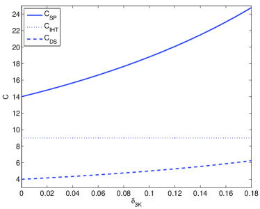
Figure 3: The constants of the SP, IHT and DS algorithms as a funtion of $\delta_{3K}$

In table I we summarize the performance guarantees of several different algorithms – the DS [8], the BP [29], and the three algorithms analyzed in this paper.

Alg.	RIP Condition	Probability of Correctness	Constant	The Obtained Bound
DS	$\delta_{2K}+\delta_{3K}\leq 1$	$1-(\sqrt{\pi(1+a)\log{N}}\cdot N^{a})^{-1}$	$\frac{4}{1-2\delta_{3K}}$	$C_{DS}^{2}\cdot(2(1+a)\log{N})\cdot K\sigma^{2}$
BP	$\delta_{2K}+3\delta_{3K}\leq 1$	$1-(N^{a})^{-1}$	$>\frac{32}{\kappa^{4}}$	$C_{BP}^{2}\cdot(2(1+a)\log{N})\cdot K\sigma^{2}$
SP	$\delta_{3K}\leq 0.139$	$1-(\sqrt{\pi(1+a)\log{N}}\cdot N^{a})^{-1}$	$\leq 21.41$	$C_{SP}^{2}\cdot(2(1+a)\log{N})\cdot K\sigma^{2}$
CoSaMP	$\delta_{4K}\leq 0.1$	$1-(\sqrt{\pi(1+a)\log{N}}\cdot N^{a})^{-1}$	$\leq 34.2$	$C_{CoSaMP}^{2}\cdot(2(1+a)\log{N})\cdot K\sigma^{2}$
IHT	$\delta_{3K}\leq\frac{1}{\sqrt{32}}$	$1-(\sqrt{\pi(1+a)\log{N}}\cdot N^{a})^{-1}$	$9$	$C_{IHT}^{2}\cdot(2(1+a)\log{N})\cdot K\sigma^{2}$

TABLE I: Near oracle performance guarantees for the DS, BP, SP, CoSaMP and IHT techniques.

We can observe the following:

1. In terms of the RIP: DS and BP are the best, then IHT, then SP and last is CoSaMP.

2. In terms of the constants in the bounds: the smallest constant is achieved by DS. Then come IHT, SP, CoSaMP and BP in this order.

3. In terms of the probability: all have the same probability except the BP which gives a weaker guarantee.

4. Though the CoSaMP has a weaker guarantee compared to the SP, it has an efficient implementation that saves the matrix inversion in the algorithm.

For completeness of the discussion here, we also refer to algorithms’ complexity: the IHT is the cheapest, CoSaMP and SP come next with a similar complexity (with a slight advantage to CoSaMP). DS and BP seem to be the most complex.

Interestingly, in the guarantees of the OMP and the thresholding in [21] better constants are obtained. However, these results, as mentioned before, holds under mutual-coherence based conditions, which are more restricting. In addition, their validity relies on the magnitude of the entries of ${\bf x}$ and the noise power, which is not correct for the results presented in this section for the greedy-like methods. Furthermore, though we get bigger constants with these methods, the conditions are not tight, as will be seen in the next section.

IV Experiments

In our experiments we use a random dictionary with entries drawn from the canonic normal distribution. The columns of the dictionary are normalized and the dimensions are $m=512$ and $N=1024$. The vector ${\bf x}$ is generated by selecting a support uniformly at random. Then the elements in the support are generated using the following model:

$${\bf x}_{i}=10\epsilon_{i}(1+\left|n_{i}\right|)$$ (IV.1)

where $\epsilon_{i}$ is $\pm 1$ with probability $0.5$, and $n_{i}$ is a canonic normal random variable. The support and the non-zero values are statistically independent. We repeat each experiment $1500$ times.

In the first experiment we calculate the error of the SP, CoSaMP and IHT methods for different sparsity levels. The noise variance is set to $\sigma=1$. Fig. 4 presents the squared-error $\left\|{\bf x}-{\bf\hat{x}}\right\|_{2}^{2}$ of all the instances of the experiment for the three algorithms. Our goal is to show that with high-probability the error obtained is bounded by the guarantees we have developed. For each algorithm we add the theoretical guarantee and the oracle performance. As can be seen, the theoretical guarantees are too loose and the actual performance of the algorithms is much better. However, we see that both the theoretical and the empirical performance curves show a proportionality to the oracle error. Note that the actual performance of the algorithms’ may be better than the oracle’s – this happens because the oracle is the Maximum-Likelihood Estimator (MLE) in this case [31], and by adding a bias one can perform even better in some cases.

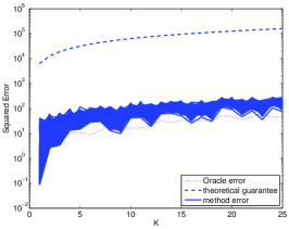
(a) SP method

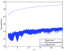
(b) CoSaMP method

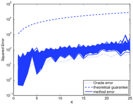
(c) IHT method

Figure 4: The squared-error as achieved by the SP, the CoSaMP and the IHT algorithms as a function of the cardinality. The graphs also show the theoretical guarantees and the oracle performance.

Fig. 5(a) presents the mean-squared-error (by averaging all the experiments) for the range where the RIP-condition seems to hold, and Fig. 5(b) presents this error for a wider range, where it is likely top be violated. It can be seen that in the average case, though the algorithms get different constants in their bounds, they achieve almost the same performance. We also see a near-linear curve describing the error as a function of $K$. Finally, we observe that the SP and the CoSaMP, which were shown to have worse constants in theory, have better performance and are more stable in the case where the RIP-condition do not hold anymore.

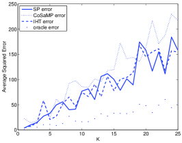
(a) RIP condition satisfied

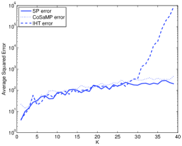
(b) RIP condition not satisfied

Figure 5: The mean-squared-error of the SP, the CoSaMP and the IHT algorithms as a function of the cardinality.

In a second experiment we calculate the error of the SP, the CoSaMP and the IHT methods for different noise variances. The sparsity is set to $K=10$. Fig. 6 presents the error of all the instances of the experiment for the three algorithms. Here as well we add the theoretical guarantee and the oracle performance. As we saw before, the guarantee is not tight but the error is proportional to the oracle estimator’s error.

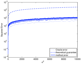
(a) SP method

(b) CoSaMP method

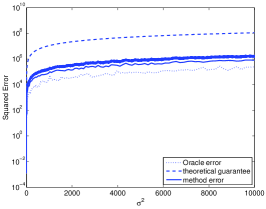
(c) IHT method

Figure 6: The squared-error as achieved by the SP, the CoSaMP and the IHT algorithms as a function of the noise variance. The graphs also show the theoretical guarantees and the oracle performance.

Fig. 7 presents the mean-squared-error as a function of the noise variance, by averaging over all the experiments. It can be seen that the error behaves linearly with respect to the variance, as expected from the theoretical analysis. Again we see that the constants are not tight and that the algorithms behave in a similar way. Finally, we note that the algorithms succeed in meeting the bounds even in very low signal-to-noise ratios, where simple greedy algorithms are expected to fail.

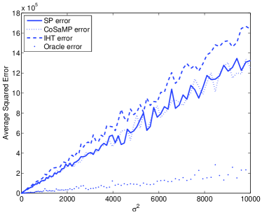
Figure 7: The mean-squared-error of the SP, the CoSaMP and the IHT algorithms as a function of the noise variance.

V Extension to the non-exact sparse case

In the case where ${\bf x}$ is not exactly $K$-sparse, our analysis has to change. Following the work reported in [13], we have the following error bounds for all algorithms (with the different RIP condition and constant).

Theorem V.1

For the SP, CoSaMP and IHT algorithms, under their appropriate RIP conditions, it holds that after at most

$$\ell^{*}=\left\lceil\log_{2}\left(\frac{\left\|{\bf x}\right\|_{2}}{\left\|{\bf D}_{T_{\bf e}}^{*}{\bf e}\right\|_{2}}\right)\right\rceil$$ (V.1)

iterations, the estimation $\hat{{\bf x}}$ gives an accuracy of the form

$$\left\|{\bf x}-\hat{{\bf x}}\right\|_{2} \leq C\bigg{(}\left\|{\bf D}_{T_{\bf e}}^{*}{\bf e}\right\|_{2}$$

$$+(1+\delta_{K})\left\|{\bf x}-{\bf x}_{K}\right\|_{2}+\frac{1+\delta_{K}}{\sqrt{K}}\left\|{\bf x}-{\bf x}_{K}\right\|_{1}\bigg{)}.$$

where ${\bf x}_{K}$ is a $K$-sparse vector that nulls all entries in ${\bf x}$ apart from the $K$ dominant ones. $C$ is the appropriate constant value, dependent on the algorithm.

If we assume that ${\bf e}$ is a white Gaussian noise with variance $\sigma^{2}$ and that the columns of ${\bf D}$ are normalized, then with probability exceeding $1-(\sqrt{\pi(1+a)\log{N}}\cdot N^{a})^{-1}$ we get that

$$\left\|{\bf x}-\hat{{\bf x}}\right\|_{2}^{2} \leq 2\cdot C^{2}\bigg{(}\sqrt{(1+a)\log{N}\cdot K}\cdot\sigma$$

$$~{}~{}~{}~{}~{}~{}~{}~{}+\left\|{\bf x}-{\bf x}_{K}\right\|_{2}+\frac{1}{\sqrt{K}}\left\|{\bf x}-{\bf x}_{K}\right\|_{2}\bigg{)}^{2}.$$

Proof: Proposition 3.5 from [13] provides us with the following claim

$$\left\|{\bf D}{\bf x}\right\|_{2}\leq\sqrt{1+\delta_{K}}\left(\left\|{\bf x}\right\|_{2}+\frac{1}{\sqrt{K}}\left\|{\bf x}\right\|_{1}\right).$$ (V.4)

When ${\bf x}$ is not exactly $K$-sparse we get that the effective error in our results becomes $\tilde{{\bf e}}={\bf e}+{\bf D}({\bf x}-{\bf x}_{K})$. Thus, using the error bounds of the algorithms with the inequality in (V.4) we get

$$\left\|{\bf x}-\hat{{\bf x}}\right\|_{2} \leq C\left\|{\bf D}_{T_{\bf e}}^{*}{\bf\tilde{e}}\right\|_{2}$$

$$\leq C\left\|{\bf D}_{T_{\bf e}}^{*}\left({\bf e}+{\bf D}({\bf x}-{\bf x}_{K})\right)\right\|_{2}$$

$$\leq C\left\|{\bf D}_{T_{\bf e}}^{*}{\bf e}\right\|+C\left\|{\bf D}_{T_{\bf e}}^{*}{\bf D}({\bf x}-{\bf x}_{K})\right\|_{2}$$

$$\leq C\left\|{\bf D}_{T_{\bf e}}^{*}{\bf e}\right\|+C\sqrt{1+\delta_{K}}\left\|{\bf D}({\bf x}-{\bf x}_{K})\right\|_{2}$$

$$\leq C\bigg{(}\left\|{\bf D}_{T_{\bf e}}^{*}{\bf e}\right\|_{2}+(1+\delta_{K})\left\|{\bf x}-{\bf x}_{K}\right\|_{2}$$

$$+\frac{1+\delta_{K}}{\sqrt{K}}\left\|{\bf x}-{\bf x}_{K}\right\|_{1}\bigg{)},$$

which proves (V.1). Using the same steps taken in Theorems III.3, III.6, and III.9, lead us to

$$\left\|{\bf x}-\hat{{\bf x}}\right\|_{2}^{2} \leq C^{2}\bigg{(}\sqrt{(2(1+a)\log{N})\cdot K}\cdot\sigma$$

$$+(1+\delta_{K})\left\|{\bf x}-{\bf x}_{K}\right\|_{2}+\frac{1+\delta_{K}}{\sqrt{K}}\left\|{\bf x}-{\bf x}_{K}\right\|_{1}\bigg{)}^{2}.$$

Since the RIP condition for all the algorithms satisfies $\delta_{K}\leq\sqrt{2}-1$, plugging this into (V) gives (V.1), and this concludes the proof. $\Box$

Just as before, we should wonder how close is this bound to the one obtained by an oracle that knows the support $T$ of the $K$ dominant entries in ${\bf x}$. Following [15], we derive an expression for such an oracle. Using the fact that the oracle is given by ${\bf D}_{T}^{\dagger}{\bf y}={\bf D}_{T}^{\dagger}({\bf D}{\bf x}_{T}+{\bf D}({\bf x}-{\bf x}_{T})+{\bf e})$, its MSE is bounded by

$$E\left\|{\bf x}-\hat{{\bf x}}_{oracle}\right\|_{2}^{2}=E\left\|{\bf x}-{\bf D}_{T}^{\dagger}{\bf y}\right\|_{2}^{2}$$ (V.7)

$$=E\left\|{\bf x}-{\bf x}_{T}-{\bf D}_{T}^{\dagger}{\bf e}-{\bf D}_{T}^{\dagger}{\bf D}({\bf x}-{\bf x}_{T})\right\|_{2}^{2}$$

$$\leq\left(\left\|{\bf x}-{\bf x}_{T}\right\|_{2}+\left\|{\bf D}_{T}^{\dagger}{\bf D}({\bf x}-{\bf x}_{T})\right\|_{2}+E\left\|{\bf D}_{T}^{\dagger}{\bf e}\right\|_{2}\right)^{2},$$

where we have used the triangle inequality. Using the relation given in (I-B) for the last term, and properties of the RIP for the second, we obtain

$$E\left\|{\bf x}-\hat{{\bf x}}_{oracle}\right\|_{2}^{2}\leq$$ (V.8)

$$~{}~{}\left(\left\|{\bf x}-{\bf x}_{T}\right\|_{2}+\frac{1}{\sqrt{1-\delta_{K}}}\left\|{\bf D}({\bf x}-{\bf x}_{T})\right\|_{2}+\frac{\sqrt{K}}{\sqrt{1-\delta_{K}}}\sigma\right)^{2}.$$

Finally, the middle-term can be further handled using (V.4), and we arrive to

$$E\left\|{\bf x}-\hat{{\bf x}}_{oracle}\right\|_{2}^{2} \leq \frac{1}{1-\delta_{k}}\bigg{(}(1+\sqrt{1+\delta_{K}})\left\|{\bf x}-{\bf x}_{T}\right\|_{2}$$

$$+\frac{\sqrt{1+\delta_{K}}}{\sqrt{K}}\left\|{\bf x}-{\bf x}_{K}\right\|_{1}+\sqrt{K}\sigma\bigg{)}^{2}.$$

Thus we see again that the error bound in the non-exact sparse case, is up to a constant and the $\log{N}$ factor the same as the one of the oracle estimator.

VI Conclusion

In this paper we have presented near-oracle performance guarantees for three greedy-like algorithms – the Subspace Pursuit, the CoSaMP, and the Iterative Hard-Thresholding. The approach taken in our analysis is an RIP-based (as opposed to mutual-coherence ones). Despite their resemblance to greedy algorithms, such as the OMP and the thresholding, our study leads to uniform guarantees for the three algorithms explored, i.e., the near-oracle error bounds are dependent only on the dictionary properties (RIP constant) and the sparsity level of the sought solution. We have also presented a simple extension of our results to the case where the representations are only approximately sparse.

Appendix A Proof of Theorem III.1 – inequality (III.1)

In the proof of (III.1) we use two main inequalities:

$$\left\|{\bf x}_{T-\tilde{T}^{\ell}}\right\|_{2} \leq \frac{2\delta_{3K}}{(1-\delta_{3K})^{2}}\left\|{\bf x}_{T-{T}^{\ell-1}}\right\|_{2}$$

$$+\frac{2}{(1-\delta_{3K})^{2}}\left\|{\bf D}_{T_{\bf e}}^{*}{\bf e}\right\|_{2},$$

and

$$\left\|{\bf x}_{T-T^{\ell}}\right\|_{2} \leq \frac{1+\delta_{3K}}{1-\delta_{3K}}\left\|{\bf x}_{T-\tilde{T}^{\ell}}\right\|_{2}$$

$$+\frac{4}{1-\delta_{3K}}\left\|{\bf D}_{T_{{\bf e}}}^{*}{\bf e}\right\|_{2}.$$

Their proofs are in Appendices B and C respectively. The inequality (III.1) is obtained by substituting (A) into (A) as shown below:

$$\left\|{\bf x}_{T-T^{\ell}}\right\|_{2} \leq \frac{1+\delta_{3K}}{1-\delta_{3K}}\left\|{\bf x}_{T-\tilde{T}^{\ell}}\right\|_{2}+\frac{4}{1-\delta_{3K}}\left\|{\bf D}_{T_{{\bf e}}}^{*}{\bf e}\right\|_{2}$$

$$\leq \frac{1+\delta_{3K}}{1-\delta_{3K}}\left[\frac{2\delta_{3K}}{(1-\delta_{3K})^{2}}\left\|{\bf x}_{T-T^{\ell-1}}\right\|_{2}\right.$$

$$\left.+\frac{2}{(1-\delta_{3K})^{2}}\left\|{\bf D}_{T_{\bf e}}^{*}{\bf e}\right\|_{2}\right]+\frac{4}{1-\delta_{3K}}\left\|{\bf D}_{T_{{\bf e}}}^{*}{\bf e}\right\|_{2}$$

$$\leq \frac{2\delta_{3K}(1+\delta_{3K})}{(1-\delta_{3K})^{3}}\left\|{\bf x}_{T-T^{\ell-1}}\right\|_{2}$$

$$+\frac{2(1+\delta_{3K})}{(1-\delta_{3K})^{3}}\left\|{\bf D}_{T_{\bf e}}^{*}{\bf e}\right\|_{2}+\frac{4}{1-\delta_{3K}}\left\|{\bf D}_{T_{{\bf e}}}^{*}{\bf e}\right\|_{2}$$

$$\leq \frac{2\delta_{3K}(1+\delta_{3K})}{(1-\delta_{3K})^{3}}\left\|{\bf x}_{T-T^{\ell-1}}\right\|_{2}$$

$$+\frac{6-6\delta_{3K}+4\delta_{3K}^{2}}{(1-\delta_{3K})^{3}}\left\|{\bf D}_{T_{\bf e}}^{*}{\bf e}\right\|_{2},$$

and this concludes this proof. $\Box$

Appendix B Proof of inequality (A)

Lemma B.1

The following inequality holds true for the SP algorithm:

$$\left\|{\bf x}_{T-\tilde{T}^{\ell}}\right\|_{2} \leq \frac{2\delta_{3K}}{(1-\delta_{3K})^{2}}\left\|{\bf x}_{T-{T}^{\ell-1}}\right\|_{2}$$

$$+\frac{2}{(1-\delta_{3K})^{2}}\left\|{\bf D}_{T_{\bf e}}^{*}{\bf e}\right\|_{2},$$

Proof: We start by the residual-update step in the SP algorithm, and exploit the relation ${\bf y}={\bf D}{\bf x}+{\bf e}={\bf D}_{T-T^{\ell-1}}{\bf x}_{T-T^{\ell-1}}+{\bf D}_{T\cap T^{\ell-1}}{\bf x}_{T\cap T^{\ell-1}}+{\bf e}$. This leads to

$${\bf y}_{r}^{\ell-1} = \operatorname{resid}({\bf y},{\bf D}_{T^{\ell-1}})$$

$$= \operatorname{resid}({\bf D}_{T-T^{\ell-1}}{\bf x}_{T-T^{\ell-1}},{\bf D}_{T^{\ell-1}})$$

$$+\operatorname{resid}({\bf D}_{T\cap T^{\ell-1}}{\bf x}_{T\cap T^{\ell-1}},{\bf D}_{T^{\ell-1}})+\operatorname{resid}({\bf e},{\bf D}_{T^{\ell-1}}).$$

Here we have used the linearity of the operator $\operatorname{resid}(\cdot,{\bf D}_{T^{\ell-1}})$ with respect to its first entry. The second term in the right-hand-side (rhs) is $0$ since ${\bf D}_{T\cap T^{\ell-1}}{\bf x}_{T\cap T^{\ell-1}}\in\operatorname{span}({\bf D}_{T^{\ell-1}})$. For the first term in the rhs we have

$$\operatorname{resid}({\bf D}_{T-T^{\ell-1}}{\bf x}_{T-T^{\ell-1}},{\bf D}_{\ell-1})$$ (B.2)

$$~{}~{}={\bf D}_{T-T^{\ell-1}}{\bf x}_{T-T^{\ell-1}}-\operatorname{proj}({\bf D}_{T-T^{\ell-1}}{\bf x}_{T-T^{\ell-1}},{\bf D}_{T^{\ell-1}})$$

$$~{}~{}={\bf D}_{T-T^{\ell-1}}{\bf x}_{T-T^{\ell-1}}+{\bf D}_{T^{\ell-1}}{\bf x}_{p,T^{\ell-1}}$$

$$~{}~{}=\left[{\bf D}_{T-T^{\ell-1}},{\bf D}_{T^{\ell-1}}\right]\left[\begin{array}[]{c}{\bf x}_{T-T^{\ell-1}}\\ {\bf x}_{p,T^{\ell-1}}\end{array}\right]\triangleq{\bf D}_{T\cup T^{\ell-1}}{\bf x}_{r}^{\ell-1},$$

where we have defined

$${\bf x}_{p,T^{\ell-1}} = -({\bf D}^{*}_{T^{\ell-1}}{\bf D}_{T^{\ell-1}})^{-1}{\bf D}^{*}_{T^{\ell-1}}{\bf D}_{T-T^{\ell-1}}{\bf x}_{T-T^{\ell-1}}.$$ (B.5)

Combining (B) and (B.2) leads to

$${\bf y}_{r}^{\ell-1}={\bf D}_{T\cup T^{\ell-1}}{\bf x}_{r}^{\ell-1}+\operatorname{resid}({\bf e},{\bf D}_{T^{\ell-1}}).$$ (B.6)

By the definition of $T_{\Delta}$ in Algorithm 1 we obtain

$$\left\|{\bf D}^{*}_{T_{\Delta}}{\bf y}_{r}^{\ell-1}\right\|_{2}\geq\left\|{\bf D}^{*}_{T}{\bf y}_{r}^{\ell-1}\right\|_{2}\geq\left\|{\bf D}^{*}_{T-T^{\ell-1}}{\bf y}_{r}^{\ell-1}\right\|_{2}$$ (B.7)

$$~{}~{}\geq\left\|{\bf D}^{*}_{T-T^{\ell-1}}{\bf D}_{T\cup T^{\ell-1}}{\bf x}_{r}^{\ell-1}\right\|_{2}$$

$$~{}~{}~{}~{}-\left\|{\bf D}^{*}_{T-T^{\ell-1}}\operatorname{resid}({\bf e},{\bf D}_{T^{\ell-1}})\right\|_{2}$$

$$~{}~{}\geq\left\|{\bf D}^{*}_{T-T^{\ell-1}}{\bf D}_{T\cup T^{\ell-1}}{\bf x}_{r}^{\ell-1}\right\|_{2}-\left\|{\bf D}^{*}_{T-T^{\ell-1}}{\bf e}\right\|_{2}$$

$$~{}~{}~{}~{}-\left\|{\bf D}^{*}_{T-T^{\ell-1}}\operatorname{proj}({\bf e},{\bf D}_{T^{\ell-1}})\right\|_{2}.$$

We will bound $\left\|{\bf D}^{*}_{T-T^{\ell-1}}\operatorname{proj}({\bf e},{\bf D}_{T^{\ell-1}})\right\|_{2}$ from above using RIP properties from Section II,

$$\left\|{\bf D}^{*}_{T-T^{\ell-1}}\operatorname{proj}({\bf e},{\bf D}_{T^{\ell-1}})\right\|_{2}$$

$$~{}~{}=\left\|{\bf D}^{*}_{T-T^{\ell-1}}{\bf D}_{T^{\ell-1}}({\bf D}_{T^{\ell-1}}^{*}{\bf D}_{T^{\ell-1}})^{-1}{\bf D}_{T^{\ell-1}}^{*}{\bf e}\right\|_{2}$$

$$~{}~{}\leq\frac{\delta_{3K}}{1-\delta_{3K}}\left\|{\bf D}_{T^{\ell-1}}^{*}{\bf e}\right\|_{2}.$$

Combining (B.7) and (B) leads to

$$\left\|{\bf D}^{*}_{T_{\Delta}}{\bf y}_{r}^{\ell-1}\right\|_{2}\geq\left\|{\bf D}^{*}_{T-T^{\ell-1}}{\bf D}_{T\cup T^{\ell-1}}{\bf x}_{r}^{\ell-1}\right\|_{2}$$ (B.9)

$$~{}~{}~{}~{}~{}~{}~{}~{}~{}~{}~{}~{}~{}~{}-\left\|{\bf D}^{*}_{T}{\bf e}\right\|_{2}-\frac{\delta_{3K}}{1-\delta_{3K}}\left\|{\bf D}_{T^{\ell-1}}^{*}{\bf e}\right\|_{2}$$

$$~{}~{}~{}~{}~{}~{}~{}~{}\geq\left\|{\bf D}^{*}_{T-T^{\ell-1}}{\bf D}_{T\cup T^{\ell-1}}{\bf x}_{r}^{\ell-1}\right\|_{2}-\frac{1}{1-\delta_{3K}}\left\|{\bf D}_{T_{\bf e}}^{*}{\bf e}\right\|_{2}.$$

By the definition of $T_{\Delta}$ and ${\bf y}_{r}^{\ell-1}$ it holds that $T_{\Delta}\cap T^{\ell-1}=\emptyset$ since ${\bf D}_{T^{\ell-1}}^{*}{\bf y}_{r}^{\ell-1}=0$. Using (B.6), the left-hand-side (lhs) of (B.9) is upper bounded by

$$\left\|{\bf D}^{*}_{T_{\Delta}}{\bf y}_{r}^{\ell-1}\right\|_{2}$$

$$\leq\left\|{\bf D}^{*}_{T_{\Delta}}{\bf D}_{T\cup T^{\ell-1}}{\bf x}_{r}^{\ell-1}\right\|_{2}+\left\|{\bf D}^{*}_{T_{\Delta}}\operatorname{resid}({\bf e},{\bf D}_{T^{\ell-1}})\right\|_{2}$$

$$\leq\left\|{\bf D}^{*}_{T_{\Delta}}{\bf D}_{T\cup T^{\ell-1}}{\bf x}_{r}^{\ell-1}\right\|_{2}+\left\|{\bf D}^{*}_{T_{\Delta}}{\bf e}\right\|_{2}$$

$$~{}~{}~{}~{}+\left\|{\bf D}^{*}_{T_{\Delta}}{\bf D}_{T^{\ell-1}}({\bf D}_{T^{\ell-1}}^{*}{\bf D}_{T^{\ell-1}})^{-1}{\bf D}_{T^{\ell-1}}^{*}{\bf e}\right\|_{2}$$

$$\leq\left\|{\bf D}^{*}_{T_{\Delta}}{\bf D}_{T\cup T^{\ell-1}}{\bf x}_{r}^{\ell-1}\right\|_{2}+\left\|{\bf D}^{*}_{T_{\Delta}}{\bf e}\right\|_{2}$$

$$~{}~{}~{}~{}+\frac{\delta_{3K}}{1-\delta_{3K}}\left\|{\bf D}_{T^{\ell-1}}^{*}{\bf e}\right\|_{2}$$

$$\leq\left\|{\bf D}^{*}_{T_{\Delta}}{\bf D}_{T\cup T^{\ell-1}}{\bf x}_{r}^{\ell-1}\right\|_{2}+\frac{1}{1-\delta_{3K}}\left\|{\bf D}^{*}_{T_{\bf e}}{\bf e}\right\|_{2}.$$

Combining (B.9) and (B) gives

$$\left\|{\bf D}^{*}_{T_{\Delta}}{\bf D}_{T\cup T^{\ell-1}}{\bf x}_{r}^{\ell-1}\right\|_{2}+\frac{2}{1-\delta_{3K}}\left\|{\bf D}_{T_{\bf e}}^{*}{\bf e}\right\|_{2}$$ (B.11)

$$~{}~{}~{}~{}~{}~{}\geq\left\|{\bf D}^{*}_{T-T^{\ell-1}}{\bf D}_{T\cup T^{\ell-1}}{\bf x}_{r}^{\ell-1}\right\|_{2}.$$

Removing the common rows in ${\bf D}^{*}_{T_{\Delta}}$ and ${\bf D}^{*}_{T-T^{\ell-1}}$ we get

$$\left\|{\bf D}^{*}_{T_{\Delta}-T}{\bf D}_{T\cup T^{\ell-1}}{\bf x}_{r}^{\ell-1}\right\|_{2}+\frac{2}{1-\delta_{3K}}\left\|{\bf D}_{T_{\bf e}}^{*}{\bf e}\right\|_{2}$$ (B.12)

$$~{}~{}~{}~{}\geq\left\|{\bf D}^{*}_{T-T^{\ell-1}-T_{\Delta}}{\bf D}_{T\cup T^{\ell-1}}{\bf x}_{r}^{\ell-1}\right\|_{2}$$

$$~{}~{}~{}~{}=\left\|{\bf D}^{*}_{T-\tilde{T}^{\ell}}{\bf D}_{T\cup T^{\ell-1}}{\bf x}_{r}^{\ell-1}\right\|_{2}.$$

The last equality is true because $T-T^{\ell-1}-T_{\Delta}=T-T^{\ell-1}-(\tilde{T}^{\ell}-T^{\ell-1})=T-\tilde{T}^{\ell}$.

Now we turn to bound the lhs and rhs terms of (B.12) from below and above, respectively. For the lhs term we exploit the fact that the supports $T_{\Delta}-T$ and $T\cup T^{\ell-1}$ are disjoint, leading to

$$\left\|{\bf D}^{*}_{T_{\Delta}-T}{\bf D}_{T\cup T^{\ell-1}}{\bf x}_{r}^{\ell-1}\right\|_{2} \leq \delta_{\left|T_{\Delta}\cup T^{\ell-1}\cup T\right|}\left\|{\bf x}^{\ell-1}_{r}\right\|_{2}$$

$$\leq \delta_{3K}\left\|{\bf x}^{\ell-1}_{r}\right\|_{2}$$

For the rhs term in (B.12), we obtain

$$\left\|{\bf D}^{*}_{T-\tilde{T}^{\ell}}{\bf D}_{T\cup T^{\ell-1}}{\bf x}_{r}^{\ell-1}\right\|_{2}$$ (B.14)

$$~{}~{}\geq\left\|{\bf D}^{*}_{T-\tilde{T}^{\ell}}{\bf D}_{T-\tilde{T}^{\ell}}({\bf x}_{r}^{\ell-1})_{T-\tilde{T}^{\ell}}\right\|_{2}$$

$$~{}~{}~{}~{}-\left\|{\bf D}^{*}_{T-\tilde{T}^{\ell}}{\bf D}_{(T\cup T^{\ell-1})-(T-\tilde{T}^{\ell})}({\bf x}_{r}^{\ell-1})_{(T\cup T^{\ell-1})-(T-\tilde{T}^{\ell})}\right\|_{2}$$

$$~{}~{}\geq(1-\delta_{K})\left\|({\bf x}_{r}^{\ell-1})_{T-\tilde{T}^{\ell}}\right\|_{2}-\delta_{3K}\left\|{\bf x}_{r}^{\ell-1}\right\|_{2}$$

$$~{}~{}\geq(1-\delta_{3K})\left\|({\bf x}_{r}^{\ell-1})_{T-\tilde{T}^{\ell}}\right\|_{2}-\delta_{3K}\left\|{\bf x}_{r}^{\ell-1}\right\|_{2}$$

Substitution of the two bounds derived above into (B.12) gives

$$2\delta_{3K}\left\|{\bf x}^{\ell-1}_{r}\right\|_{2}+\frac{2}{1-\delta_{3K}}\left\|{\bf D}_{T_{\bf e}}^{*}{\bf e}\right\|_{2}$$ (B.15)

$$~{}~{}~{}~{}~{}~{}\geq(1-\delta_{3K})\left\|({\bf x}_{r}^{\ell-1})_{T-\tilde{T}^{\ell}}\right\|_{2}.$$

The above inequality uses ${\bf x}^{\ell-1}_{r}$, which was defined in (B.2), and this definition relies on yet another one definition for the vector ${\bf x}_{p,T^{\ell-1}}$ in (B.5). We proceed by bounding $\left\|{\bf x}_{p,T^{\ell-1}}\right\|_{2}$ from above,

$$\left\|{\bf x}_{p,T^{\ell-1}}\right\|_{2}$$ (B.16)

$$~{}~{}=\left\|-({\bf D}^{*}_{T^{\ell-1}}{\bf D}_{T^{\ell-1}})^{-1}{\bf D}^{*}_{T^{\ell-1}}{\bf D}_{T-T^{\ell-1}}{\bf x}_{T-T^{\ell-1}}\right\|_{2}$$

$$~{}~{}\leq\frac{1}{1-\delta_{K}}\left\|-{\bf D}^{*}_{T^{\ell-1}}{\bf D}_{T-T^{\ell-1}}{\bf x}_{T-T^{\ell-1}}\right\|_{2}$$

$$~{}~{}\leq\frac{\delta_{2K}}{1-\delta_{K}}\left\|{\bf x}_{T-T^{\ell-1}}\right\|_{2}\leq\frac{\delta_{3K}}{1-\delta_{3K}}\left\|{\bf x}_{T-T^{\ell-1}}\right\|_{2},$$

and get

$$\left\|{\bf x}_{r}^{\ell-1}\right\|_{2} \leq \left\|{\bf x}_{T-T^{\ell-1}}\right\|_{2}+\left\|{\bf x}_{p,T^{\ell-1}}\right\|_{2}$$

$$\leq \left(1+\frac{\delta_{3K}}{1-\delta_{3K}}\right)\left\|{\bf x}_{T-T^{\ell-1}}\right\|_{2}$$

$$\leq \frac{1}{1-\delta_{3K}}\left\|{\bf x}_{T-T^{\ell-1}}\right\|_{2}.$$

In addition, since $({\bf x}_{r}^{\ell-1})_{T-T^{\ell-1}}={\bf x}_{T-T^{\ell-1}}$ then $({\bf x}_{r}^{\ell-1})_{T-\tilde{T}^{\ell}}={\bf x}_{T-\tilde{T}^{\ell}}$. Using this fact and (B) with (B.15) leads to

$$\left\|{\bf x}_{T-\tilde{T}^{\ell}}\right\|_{2}$$ (B.18)

$$~{}~{}\leq\frac{2\delta_{3K}}{(1-\delta_{3K})^{2}}\left\|{\bf x}_{T-{T}^{\ell-1}}\right\|_{2}+\frac{2}{(1-\delta_{3K})^{2}}\left\|{\bf D}_{T_{\bf e}}^{*}{\bf e}\right\|_{2},$$

which proves the inequality in (A). $\Box$

Appendix C Proof of inequality (A)

Lemma C.1

The following inequality holds true for the SP algorithm:

$$\left\|{\bf x}_{T-T^{\ell}}\right\|_{2} \leq \frac{1+\delta_{3K}}{1-\delta_{3K}}\left\|{\bf x}_{T-\tilde{T}^{\ell}}\right\|_{2}+\frac{4}{1-\delta_{3K}}\left\|{\bf D}_{T_{{\bf e}}}^{*}{\bf e}\right\|_{2}.$$

Proof: We will define the smear vector ${\boldsymbol{\epsilon}}={\bf x}_{p}-{\bf x}_{\tilde{T}^{\ell}}$, where ${\bf x}_{p}$ is the outcome of the representation computation over ${\tilde{T}}^{\ell}$, given by

$${\bf x_{p}}={\bf D}_{\tilde{T}^{\ell}}^{\dagger}{\bf y}={\bf D}_{\tilde{T}^{\ell}}^{\dagger}({\bf D}_{T}{\bf x}_{T}+{\bf e}),$$ (C.1)

as defined in Algorithm 1. Expanding the first term in the last equality gives:

$${\bf D}_{\tilde{T}^{\ell}}^{\dagger}{\bf D}_{T}{\bf x}_{T}={\bf D}_{\tilde{T}^{\ell}}^{\dagger}{\bf D}_{T\cap\tilde{T}^{\ell}}{\bf x}_{T\cap\tilde{T}^{\ell}}+{\bf D}_{\tilde{T}^{\ell}}^{\dagger}{\bf D}_{T-\tilde{T}^{\ell}}{\bf x}_{T-\tilde{T}^{\ell}}$$ (C.2)

$$~{}={\bf D}_{\tilde{T}^{\ell}}^{\dagger}\left[{\bf D}_{T\cap\tilde{T}^{\ell}},{\bf D}_{\tilde{T}^{\ell}-T}\right]\left[\begin{array}[]{c}{\bf x}_{T\cap\tilde{T}^{\ell}}\\ {\bf 0}\end{array}\right]+{\bf D}_{\tilde{T}^{\ell}}^{\dagger}{\bf D}_{T-\tilde{T}^{\ell}}{\bf x}_{T-\tilde{T}^{\ell}}$$ (C.5)

$$~{}={\bf D}_{\tilde{T}^{\ell}}^{\dagger}{\bf D}_{\tilde{T}^{\ell}}{\bf x}_{\tilde{T}^{\ell}}+{\bf D}_{\tilde{T}^{\ell}}^{\dagger}{\bf D}_{T-\tilde{T}^{\ell}}{\bf x}_{T-\tilde{T}^{\ell}}$$

$$~{}={\bf x}_{\tilde{T}^{\ell}}+{\bf D}_{\tilde{T}^{\ell}}^{\dagger}{\bf D}_{T-\tilde{T}^{\ell}}{\bf x}_{T-\tilde{T}^{\ell}}.$$

The equalities hold based on the definition of ${\bf D}_{\tilde{T}^{\ell}}^{\dagger}$ and on the fact that ${\bf x}$ is $0$ outside of $T$. Using (C.2) we bound the smear energy from above, obtaining

$$\left\|{\boldsymbol{\epsilon}}\right\|_{2} \leq \left\|{\bf D}_{\tilde{T}^{\ell}}^{\dagger}{\bf D}_{T}{\bf x}_{T}\right\|_{2}+\left\|{\bf D}_{\tilde{T}^{\ell}}^{\dagger}{\bf e}\right\|_{2}$$

$$= \left\|({\bf D}_{\tilde{T}^{\ell}}^{*}{\bf D}_{\tilde{T}^{\ell}})^{-1}{\bf D}_{\tilde{T}^{\ell}}^{*}{\bf D}_{T-\tilde{T}^{\ell}}{\bf x}_{T-\tilde{T}^{\ell}}\right\|_{2}$$

$$+\left\|({\bf D}_{\tilde{T}^{\ell}}^{*}{\bf D}_{\tilde{T}^{\ell}})^{-1}{\bf D}_{\tilde{T}^{\ell}}^{*}{\bf e}\right\|_{2}$$

$$\leq \frac{\delta_{3K}}{1-\delta_{3K}}\left\|{\bf x}_{T-\tilde{T}^{\ell}}\right\|_{2}+\frac{1}{1-\delta_{3K}}\left\|{\bf D}_{\tilde{T}^{\ell}}^{*}{\bf e}\right\|_{2}.$$

We now turn to bound $\left\|{\boldsymbol{\epsilon}}\right\|_{2}$ from below. We denote the support of the $K$ smallest coefficients in ${\bf x}_{p}$ by $\Delta T\triangleq\tilde{T}^{\ell}-T^{\ell}$. Thus, for any set $T^{\prime}\subset\tilde{T}^{\ell}$ of cardinality $K$, it holds that $\left\|({\bf x}_{p})_{\Delta T}\right\|_{2}\leq\left\|({\bf x}_{p})_{T^{\prime}}\right\|_{2}$. In particular, we shall choose $T^{\prime}$ such that $T^{\prime}\cap T=\emptyset$, which necessarily exists because $\tilde{T}^{\ell}$ is of cardinality $2K$ and therefore there must be at $K$ entries in this support that are outside $T$. Thus, using the relation ${\boldsymbol{\epsilon}}={\bf x}_{p}-{\bf x}_{\tilde{T}^{\ell}}$ we get

$$\left\|({\bf x}_{p})_{\Delta T}\right\|_{2} \leq \left\|({\bf x}_{p})_{T^{\prime}}\right\|_{2}=\left\|\left({\bf x}_{\tilde{T}^{\ell}}\right)_{T^{\prime}}+{\boldsymbol{\epsilon}}_{T^{\prime}}\right\|_{2}$$

$$= \left\|{\boldsymbol{\epsilon}}_{T^{\prime}}\right\|_{2}\leq\left\|{\boldsymbol{\epsilon}}\right\|_{2}.$$

Because ${\bf x}$ is supported on $T$ we have that $\left\|{\bf x}_{\Delta T}\right\|_{2}=\left\|{\bf x}_{\Delta T\cap T}\right\|_{2}$. An upper bound for this vector is reached by

$$\left\|{\bf x}_{\Delta T\cap T}\right\|_{2} = \left\|({\bf x}_{p})_{\Delta T\cap T}-{\boldsymbol{\epsilon}}_{\Delta T\cap T}\right\|_{2}$$

$$\leq \left\|({\bf x}_{p})_{\Delta T\cap T}\right\|_{2}+\left\|{\boldsymbol{\epsilon}}_{\Delta T\cap T}\right\|_{2}$$

$$\leq \left\|({\bf x}_{p})_{\Delta T}\right\|_{2}+\left\|{\boldsymbol{\epsilon}}\right\|_{2}\leq 2\left\|{\boldsymbol{\epsilon}}\right\|_{2},$$

where the last step uses (C). The vector ${\bf x}_{T-T^{\ell}}$ can be decomposed as ${\bf x}_{T-T^{\ell}}=\left[{\bf x}_{T\cap\Delta T}^{*},{\bf x}^{*}_{T-\tilde{T}^{\ell}}\right]^{*}$. Using (C) and (C) we get

$$\left\|{\bf x}_{T-T^{\ell}}\right\|_{2}\leq\left\|{\bf x}_{T\cap\Delta T}\right\|_{2}+\left\|{\bf x}_{T-\tilde{T}^{\ell}}\right\|_{2}\leq 2\left\|{\boldsymbol{\epsilon}}\right\|_{2}+\left\|{\bf x}_{T-\tilde{T}^{\ell}}\right\|_{2}$$

$$~{}~{}\leq\left(1+\frac{2\delta_{3K}}{1-\delta_{3K}}\right)\left\|{\bf x}_{T-\tilde{T}^{\ell}}\right\|_{2}+\frac{2}{1-\delta_{3K}}\left\|{\bf D}_{\tilde{T}^{\ell}}^{*}{\bf e}\right\|_{2}$$

$$~{}~{}=\frac{1+\delta_{3K}}{1-\delta_{3K}}\left\|{\bf x}_{T-\tilde{T}^{\ell}}\right\|_{2}+\frac{4}{1-\delta_{3K}}\left\|{\bf D}_{T_{{\bf e}}}^{*}{\bf e}\right\|_{2},$$

where the last step uses the property $\left\|{\bf D}_{{\tilde{T}}^{\ell}}^{*}{\bf e}\right\|_{2}\leq 2\left\|{\bf D}_{T_{{\bf e}}}^{*}{\bf e}\right\|_{2}$ taken from Section II, and this concludes the proof. $\Box$

Appendix D Proof of inequality (III.4)

Lemma D.1

The following inequality holds true for the CoSaMP algorithm:

$$\left\|{\bf x}-\hat{{\bf x}}_{CoSaMP}^{\ell}\right\|_{2}\leq\frac{4\delta_{4K}}{(1-\delta_{4K})^{2}}\left\|{\bf x}-\hat{{\bf x}}_{CoSaMP}^{\ell-1}\right\|_{2}+\frac{14-6\delta_{4K}}{(1-\delta_{4K})^{2}}\left\|{\bf D}_{T_{{\bf e}}}^{*}{\bf e}\right\|_{2}.$$

Proof: We denote $\hat{{\bf x}}_{CoSaMP}^{\ell}$ as the solution of CoSaMP in the $\ell$-th iteration: $\hat{{\bf x}}_{CoSaMP,(T^{\ell})^{C}}^{\ell}=0$ and $\hat{{\bf x}}_{CoSaMP,T^{\ell}}^{\ell}=({\bf x}_{p})_{T^{\ell}}$. We further define ${\bf r}^{\ell}\triangleq{\bf x}-\hat{{\bf x}}_{CoSaMP}^{\ell}$ and use the definition of $T_{{\bf e},p}$ (Section II). Our proof is based on the proof of Theorem 4.1 and the Lemmas used with it [13].

Since we choose $T_{\Delta}$ to contain the biggest $2K$ elements in ${\bf D}^{*}{\bf y}_{r}^{\ell}$ and $\left|T^{\ell-1}\cup T\right|\leq 2K$ it holds true that $\left\|({\bf D}^{*}{\bf y}_{r}^{\ell})_{T^{\ell}\cup T}\right\|_{2}\leq\left\|({\bf D}^{*}{\bf y}_{r}^{\ell})_{T_{\Delta}}\right\|_{2}$. Removing the common elements from both sides we get

$$\left\|({\bf D}^{*}{\bf y}_{r}^{\ell})_{(T^{\ell}\cup T)-T_{\Delta}}\right\|_{2}\leq\left\|({\bf D}^{*}{\bf y}_{r}^{\ell})_{T_{\Delta}-(T^{\ell}\cup T)}\right\|_{2}.$$ (D.1)

We proceed by bounding the rhs and lhs of (D.1), from above and from below respectively, using the triangle inequality. We use Propositions II.1 and II.2, the definition of $T_{{\bf e},2}$, and the fact that $\left\|{\bf r}^{\ell}\right\|_{2}=\left\|{\bf r}_{T^{\ell}\cup T}^{\ell}\right\|_{2}$ (this holds true since the support of ${\bf r}^{\ell}$ is over $T\cup T^{\ell}$). For the rhs we obtain

$$\left\|({\bf D}^{*}{\bf y}_{r}^{\ell})_{T_{\Delta}-(T^{\ell}\cup T)}\right\|_{2} = \left\|{\bf D}^{*}_{T_{\Delta}-(T^{\ell}\cup T)}({\bf D}{\bf r}^{\ell}+{\bf e})\right\|_{2}$$

$$\leq \left\|{\bf D}^{*}_{T_{\Delta}-(T^{\ell}\cup T)}{\bf D}_{T^{\ell}\cup T}{\bf r}_{T^{\ell}\cup T}^{\ell}\right\|_{2}+\left\|{\bf D}^{*}_{T_{\Delta}-(T^{\ell}\cup T)}{\bf e}\right\|_{2}$$

$$\leq \delta_{4K}\left\|{\bf r}^{\ell}\right\|_{2}+\left\|{\bf D}^{*}_{T_{{\bf e},2}}{\bf e}\right\|_{2}.$$

and for the lhs:

$$\left\|({\bf D}^{*}{\bf y}_{r}^{\ell})_{(T^{\ell}\cup T)-T_{\Delta}}\right\|_{2} = \left\|{\bf D}^{*}_{(T^{\ell}\cup T)-T_{\Delta}}({\bf D}{\bf r}^{\ell}+{\bf e})\right\|_{2}$$

$$\geq \left\|{\bf D}^{*}_{(T^{\ell}\cup T)-T_{\Delta}}{\bf D}_{(T^{\ell}\cup T)-T_{\Delta}}{\bf r}^{\ell}_{(T^{\ell}\cup T)-T_{\Delta}}\right\|_{2}$$

$$-\left\|{\bf D}^{*}_{(T^{\ell}\cup T)-T_{\Delta}}{\bf D}_{T_{\Delta}}{\bf r}^{\ell}_{T_{\Delta}}\right\|_{2}-\left\|{\bf D}^{*}_{(T^{\ell}\cup T)-T_{\Delta}}{\bf e}\right\|_{2}$$

$$\geq (1-\delta_{2K})\left\|{\bf r}^{\ell}_{(T^{\ell}\cup T)-T_{\Delta}}\right\|_{2}-\delta_{4K}\left\|{\bf r}^{\ell}_{T_{\Delta}}\right\|_{2}-\left\|{\bf D}^{*}_{T_{{\bf e},2}}{\bf e}\right\|_{2}.$$

Because ${\bf r}^{\ell}$ is supported over $T\cup T^{\ell}$, it holds true that $\left\|{\bf r}^{\ell}_{(T\cup T^{\ell})-T_{\Delta}}\right\|_{2}=\left\|{\bf r}^{\ell}_{T_{\Delta}^{C}}\right\|_{2}$. Combining (D) and (D) with (D.1), gives

$$\left\|{\bf r}^{\ell}_{T_{\Delta}^{C}}\right\|_{2} \leq \frac{2\delta_{4K}\left\|{\bf r}^{\ell}\right\|_{2}+2\left\|{\bf D}_{T_{{\bf e},2}}^{*}{\bf e}\right\|_{2}}{1-\delta_{2K}}$$

$$\leq \frac{2\delta_{4K}\left\|{\bf r}^{\ell}\right\|_{2}+4\left\|{\bf D}_{T_{{\bf e}}}^{*}{\bf e}\right\|_{2}}{1-\delta_{4K}}.$$

For brevity of notations, we denote hereafter ${\tilde{T}}^{\ell}$ as ${\tilde{T}}$. Using ${\bf y}={\bf D}{\bf x}+{\bf e}={\bf D}_{\tilde{T}}{\bf x}_{\tilde{T}}+{\bf D}_{\tilde{T}^{C}}{\bf x}_{\tilde{T}^{C}}+{\bf e}$, we observe that

$$\left\|{\bf x}_{\tilde{T}}-({\bf x}_{p})_{\tilde{T}}\right\|_{2} = \left\|{\bf x}_{\tilde{T}}-{\bf D}_{\tilde{T}}^{\dagger}\left({\bf D}_{\tilde{T}}{\bf x}_{\tilde{T}}+{\bf D}_{\tilde{T}^{C}}{\bf x}_{\tilde{T}^{C}}+{\bf e}\right)\right\|_{2}$$

$$= \left\|{\bf D}_{\tilde{T}}^{\dagger}\left({\bf D}_{\tilde{T}^{C}}{\bf x}_{\tilde{T}^{C}}+{\bf e}\right)\right\|_{2}$$

$$\leq \left\|({\bf D}_{\tilde{T}}^{*}{\bf D}_{\tilde{T}})^{-1}{\bf D}_{\tilde{T}}^{*}{\bf D}_{\tilde{T}^{C}}{\bf x}_{\tilde{T}^{C}}\right\|_{2}+\left\|({\bf D}_{\tilde{T}}^{*}{\bf D}_{\tilde{T}})^{-1}{\bf D}_{\tilde{T}}^{*}{\bf e}\right\|_{2}$$

$$\leq \frac{1}{1-\delta_{3K}}\left\|{\bf D}_{\tilde{T}}^{*}{\bf D}_{\tilde{T}^{C}}{\bf x}_{\tilde{T}^{C}}\right\|_{2}+\frac{1}{1-\delta_{3K}}\left\|{\bf D}_{T_{{\bf e},3}}^{*}{\bf e}\right\|_{2}$$

$$\leq \frac{\delta_{4K}}{1-\delta_{4K}}\left\|{\bf x}_{\tilde{T}^{C}}\right\|_{2}+\frac{3}{1-\delta_{4K}}\left\|{\bf D}_{T_{{\bf e}}}^{*}{\bf e}\right\|_{2},$$

where the last inequality holds true because of Proposition II.4 and that $|\tilde{T}|=3K$. Using the triangle inequality and the fact that ${\bf x}_{p}$ is supported on ${\tilde{T}}$, we obtain

$$\left\|{\bf x}-{\bf x}_{p}\right\|_{2}\leq\left\|{\bf x}_{\tilde{T}^{C}}\right\|_{2}+\left\|{\bf x}_{\tilde{T}}-({\bf x}_{p})_{\tilde{T}}\right\|_{2},$$ (D.6)

which leads to

$$\left\|{\bf x}-{\bf x}_{p}\right\|_{2} \leq \left(1+\frac{\delta_{4K}}{1-\delta_{4K}}\right)\left\|{\bf x}_{\tilde{T}^{C}}\right\|_{2}+\frac{3}{1-\delta_{4K}}\left\|{\bf D}_{T_{{\bf e}}}^{*}{\bf e}\right\|_{2}$$

$$= \frac{1}{1-\delta_{4K}}\left\|{\bf x}_{\tilde{T}^{C}}\right\|_{2}+\frac{3}{1-\delta_{4K}}\left\|{\bf D}_{T_{{\bf e}}}^{*}{\bf e}\right\|_{2}.$$

Having the above results we can obtain (III.4) by

$$\left\|{\bf x}-\hat{{\bf x}}_{CoSaMP}^{\ell}\right\|_{2} \leq 2\left\|{\bf x}-{\bf x}_{p}\right\|_{2}$$

$$\leq 2\left(\frac{1}{1-\delta_{4K}}\left\|{\bf x}_{\tilde{T}^{C}}\right\|_{2}+\frac{3}{1-\delta_{4K}}\left\|{\bf D}_{T_{{\bf e}}}^{*}{\bf e}\right\|_{2}\right)$$

$$\leq \frac{2}{1-\delta_{4K}}\left\|{\bf r}^{\ell-1}_{T_{\Delta}^{C}}\right\|_{2}+\frac{6}{1-\delta_{4K}}\left\|{\bf D}_{T_{{\bf e}}}^{*}{\bf e}\right\|_{2}$$

$$\leq \frac{2}{1-\delta_{4K}}\left(\frac{2\delta_{4K}}{1-\delta_{4K}}\left\|{\bf r}^{\ell-1}\right\|_{2}+\frac{4}{1-\delta_{4K}}\left\|{\bf D}_{T_{{\bf e}}}^{*}{\bf e}\right\|_{2}\right)+\frac{6}{1-\delta_{4K}}\left\|{\bf D}_{T_{{\bf e}}}^{*}{\bf e}\right\|_{2}$$

$$= \frac{4\delta_{4K}}{(1-\delta_{4K})^{2}}\left\|{\bf r}^{\ell-1}\right\|_{2}+\frac{14-6\delta_{4K}}{(1-\delta_{4K})^{2}}\left\|{\bf D}_{T_{{\bf e}}}^{*}{\bf e}\right\|_{2},$$

where the inequalities are based on Lemma 4.5 from [13], (D), Lemma 4.3 from [13] and (D) respectively. $\Box$

References

• [1] D. L. Donoho, M. Elad, and V. N. Temlyakov, “Stable recovery of sparse overcomplete representations in the presence of noise,” IEEE Trans. Inf. Theory, vol. 52, no. 1, pp. 6–18, Jan. 2006.
• [2] D. L. Donoho and M. Elad, “On the stability of the basis pursuit in the presence of noise,” Signal Process., vol. 86, no. 3, pp. 511–532, 2006.
• [3] J. Tropp, “Just relax: Convex programming methods for identifying sparse signals,” IEEE Trans. Inf. Theory, vol. 52, no. 3, pp. 1030–1051, Mar. 2006.
• [4] A. M. Bruckstein, D. L. Donoho, and M. Elad, “From sparse solutions of systems of equations to sparse modeling of signals and images,” SIAM Review, vol. 51, no. 1, pp. 34–81, 2009.
• [5] B. Natarajan, “Sparse approximate solutions to linear systems,” SIAM Journal on Computing, vol. 24, pp. 227–234, 1995.
• [6] S. S. Chen, D. L. Donoho, and M. A. Saunders, “Atomic decomposition by basis pursuit,” SIAM Journal on Scientific Computing, vol. 20, no. 1, pp. 33–61, 1998.
• [7] R. Tibshirani, “Regression shrinkage and selection via the lasso,” J. Roy. Statist. Soc. B, vol. 58, no. 1, pp. 267–288, 1996.
• [8] E. J. Candès and T. Tao, “The dantzig selector: Statistical estimation when p is much larger than n,” Annals Of Statistics, vol. 35, p. 2313, 2007.
• [9] S. Chen, S. A. Billings, and W. Luo, “Orthogonal least squares methods and their application to non-linear system identification,” International Journal of Control, vol. 50, no. 5, pp. 1873–1896, 1989.
• [10] S. Mallat and Z. Zhang, “Matching pursuits with time-frequency dictionaries,” IEEE Trans. Signal Process., vol. 41, pp. 3397–3415, 1993.
• [11] G. Davis, S. Mallat, and M. Avellaneda, “Adaptive greedy approximations,” Journal of Constructive Approximation, vol. 50, pp. 57–98, 1997.
• [12] D. Needell and R. Vershynin, “Signal recovery from incomplete and inaccurate measurements via regularized orthogonal matching pursuit,” IEEE Journal of Selected Topics in Signal Processing, vol. 4, no. 2, pp. 310 –316, april 2010.
• [13] D. Needell and J. Tropp, “Cosamp: Iterative signal recovery from incomplete and inaccurate samples,” Applied and Computational Harmonic Analysis, vol. 26, no. 3, pp. 301 – 321, 2009.
• [14] W. Dai and O. Milenkovic, “Subspace pursuit for compressive sensing signal reconstruction,” IEEE Trans. Inf. Theory, vol. 55, no. 5, pp. 2230–2249, 2009.
• [15] T. Blumensath and M. E. Davies, “Iterative hard thresholding for compressed sensing,” Applied and Computational Harmonic Analysis, vol. 27, no. 3, pp. 265 – 274, 2009.
• [16] D. L. Donoho and X. Huo, “Uncertainty principles and ideal atomic decomposition,” IEEE Trans. Inf. Theory, vol. 47, no. 7, pp. 2845–2862, Nov 2001.
• [17] M. Elad and A. Bruckstein, “A generalized uncertainty principle and sparse representation in pairs of bases,” IEEE Trans. Inf. Theory, vol. 48, no. 9, pp. 2558–2567, Sep 2002.
• [18] D. L. Donoho and M. Elad, “Optimal sparse representation in general (nonorthogoinal) dictionaries via l1 minimization,” Proceedings of the National Academy of Science, vol. 100, pp. 2197–2202, Mar 2003.
• [19] E. J. Candès and T. Tao, “Near-optimal signal recovery from random projections: Universal encoding strategies?” IEEE Trans. Inf. Theory, vol. 52, no. 12, pp. 5406 –5425, dec. 2006.
• [20] E. Candès and T. Tao, “Decoding by linear programming,” IEEE Trans. Inf. Theory, vol. 51, no. 12, pp. 4203 – 4215, dec. 2005.
• [21] Z. Ben-Haim, Y. C. Eldar, and M. Elad, “Coherence-based performance guarantees for estimating a sparse vector under random noise,” to appear in IEEE Trans. Signal Process., 2010.
• [22] M. Rudelson and R. Vershynin, “Sparse reconstruction by convex relaxation: Fourier and gaussian measurements,” in Information Sciences and Systems, 2006 40th Annual Conference on, 22-24 2006, pp. 207 –212.
• [23] J. Tropp, “Just relax: convex programming methods for identifying sparse signals in noise,” IEEE Trans. Inf. Theory, vol. 52, no. 3, pp. 1030–1051, March 2006.
• [24] E. J. Candès, J. K. Romberg, and T. Tao, “Stable signal recovery from incomplete and inaccurate measurements,” Communications on Pure and Applied Mathematics, vol. 59, no. 8, pp. 1207–1223, 2006.
• [25] E. Candès, “The restricted isometry property and its implications for compressed sensing,” Comptes Rendus Mathematique, vol. 346, no. 9-10, pp. 589 – 592, 2008.
• [26] T. Cai, L. Wang, and G. Xu, “Shifting inequality and recovery of sparse signals,” IEEE Trans. Signal Process., vol. 58, no. 3, pp. 1300 –1308, march 2010.
• [27] ——, “New bounds for restricted isometry constants,” To appear in IEEE Trans. Inf. Theory., 2010.
• [28] E. J. Candès, “Modern statistical estimation via oracle inequalities,” Acta Numerica, vol. 15, pp. 257–325, 2006.
• [29] P. J. Bickel, Y. Ritov, and A. B. Tsybakov, “Simultaneous analysis of lasso and dantzig selector,” Annals of Statistics, vol. 37, no. 4, pp. 1705–1732, 2009.
• [30] T. Cai, L. Wang, and G. Xu, “Stable recovery of sparse signals and an oracle inequality,” to appear in IEEE Transactions on Information Theory, 2009. [Online]. Available: www-stat.wharton.upenn.edu/ tcai/paper/Stable-Recovery-MIP.pdf
• [31] Z. Ben-Haim and Y. C. Eldar, “The Cramèr–-Rao bound for estimating a sparse parameter vector,” IEEE Trans. Signal Process., vol. 58, no. 6, pp. 3384 –3389, june 2010.