Radiatively Induced Non Linearity in the Walecka Model

Abstract

We evaluate the effective potential for the conventional linear Walecka non perturbatively up to one loop. This quantity is then renormalized with a prescription which allows finite vacuum contributions to the three as well as four 1PI Green’s functions to survive. These terms, which are absent in the standard relativistic Hartree approximation, have a logarithmic energy scale dependence that can be tuned so as to mimic the effects of $\phi^{3}$ and $\phi^{4}$ type of terms present in the non linear Walecka model improving quantities such as the compressibility modulus and the effective nucleon mass, at saturation, by considering energy scales which are very close to the nucleon mass at vanishing density.

I Introduction

Quantum hadrodynamics (QHD) is an effective relativistic quantum field theory, based on mesons and baryons, which can be used at hadronic energy scales where the fundamental theory of strong interactions, quantum chromodynamics (QCD), presents a highly nonlinear behavior. The Walecka model waleckaANP to be considered here represents QHD by means of a lagrangian density formulated so as to describe nucleons interacting through the exchange of an isoscalar vector meson ($\omega$) as well as of a scalar-isoscalar meson ($\phi$) which is introduced to simulate intermediate range attraction due to the $s$-wave isoscalar pion pairs. The original Walecka model (QHD-I) is described by the lagrangian density

$${\cal L}={\bar{\psi}}[\gamma_{\mu}\left(i\partial^{\mu}-g_{v}V^{\mu})-(M-g_{s}\phi)\right]\psi+\frac{1}{2}(\partial_{\mu}\phi\partial^{\mu}\phi-m_{s}^{2}\phi^{2})-\frac{1}{4}F_{\mu\nu}F^{\mu\nu}+\frac{1}{2}m_{v}^{2}V_{\mu}V^{\mu}-U(\phi,V)+{\cal L}_{\rm CT}\;,$$ (1)

where $\psi$, $\phi$ and $\omega$ denote respectively baryon, scalar and vector meson fields (with the latter being coupled to a conserved baryonic current). The term $U(\phi,V)$, which describes mesonic self interactions was set to zero in the original model so as to minimize the many body effects while the term ${\cal L}_{\rm CT}$ represents the counterterms needed to eliminate any potential ultra violet divergences arising from vacuum computations.

It is important to recall that, roughly, counterterms are composed by two distinct parts the first being a divergent piece which exactly eliminates the divergence resulting from the evaluation of a Green function at a given order in perturbation theory. The second piece is composed by a finite part which is arbitrary and can be fixed by choosing an appropriated renormalization scheme ramond .

The important parameters are the ratios of coupling to masses, $C^{2}_{s}$ and $C^{2}_{v}$, with $C_{i}^{2}=(g_{i}M/m_{i})^{2}$ which are tuned to fit the saturation density $\rho_{0}=0.193\,{\rm fm}^{-3}$ and binding energy per nucleon, $BE=-15.75\,{\rm MeV}$ waleckaANP . However, the QHD-I predictions for some other relevant static properties of nuclear matter do not agree well with the values quoted in the literature. For example, using the Mean Field Approximation (MFA) which considers only in medium contributions at the one loop level one obtains that, at saturation, the effective nucleon mass is $M^{*}_{\rm sat}\sim 0.56\,M$, which is somewhat low, while the compression modulus, $K\sim 540\,{\rm MeV}$, is too high. In principle, since this is a renormalizable quantum field theory, vacuum contributions (and potential ultra violet divergences) can be properly treated yielding meaningful finite results. These contributions were first considered by Chin chin , at the one loop level, in the so called Relativistic Hartree Approximation (RHA) which produced a more reasonable value for the effective mass, $M^{*}_{\rm sat}\sim 0.72\,M$. However, the compression modulus remained at a high value, $K\sim 470\,{\rm MeV}$.

One could then try to improve the situation by also considering exchange contributions since both, MFA and RHA, consider only direct terms in a nonperturbative way. When vacuum contributions are neglected this approximation is known as the Hartree-Fock (HF) approximation producing $M^{*}_{\rm sat}\sim 0.53\,M$ and $K\sim 585\,{\rm MeV}$ waleckaANP . By comparing the results from MFA, RHA and HF one sees how vacuum effects can improve the values of $M^{*}_{\rm sat}$ and $K$. Then, the natural question is if the situation could be further improved by considering the vacuum in HF type of evaluations. The main concern now being the difficulty to deal with overall, nested, and overlapping type of divergences which surely arise due to the self consistent procedure.

The complete evaluation of vacuum contributions within direct and exchange terms was performed by Furnstahl, Perry and Serot furnstahl1 (see Ref. early for an early attempt in which only the propagators have been fully renormalized ). This cumbersome calculation considers the nonperturbative evaluation and renormalization of the energy density up to the two loop level showing the non convergence of the loop expansion. Later, the situation has been addressed with the alternative Optimized Perturbation Theory (OPT) which allows for an easier manipulation of divergences ijmpe . Two loop contributions have been evaluated and renormalized in a perturbative fashion with nonperturbative results further generated via a variational criterion. However, saturation of nuclear matter could not be achieved with the results supporting those of Ref. furnstahl1 .

Meanwhile, the compressibility modulus problem has been circumvented by introducing some more parameters, in the form of new couplings bogutabodmer , to the original Walecka model. One then considers $U(\phi,V)$ appearing in Eq. (1) as

$$U(\phi)=\frac{\kappa}{3!}\phi^{3}+\frac{\lambda}{4!}\phi^{4}\,,$$ (2)

where $\kappa=2bMg_{s}^{3}$ and $\lambda=6cg_{s}^{4}$. This version of QHD is known as the nonlinear Walecka model (NLWM) and the main role of the two additional parameters, $b$ and $c$, is to bring the compression modulus of nuclear matter and the nucleon effective mass under control. However, one may object to this course of action since the mesonic self interactions will increase the many body effects apart from increasing the parameter space. Notice also that terms like $\phi^{n}$ ($n\geq 5$) are not allowed since then, in 3+1 dimensions, one would need to introduce coupling parameters with negative mass dimensions spoiling the renormalizability of the original model. apart from increasing the parameter space.

Heide and Rudaz rudaz have then realized that it is still possible to keep $U(\phi,V)=0$ while improving both $K$ and $M^{*}_{\rm sat}$. The key ingredient in their approach is related to the complete evaluation (regularization and renormalization) of divergent vacuum contributions. Regularization is a formal way to isolate the divergences associated with a physical quantity for which many different prescriptions exist, e.g., sharp cut-off, Pauli-Villars, and Dimensional Regularization (DR). Within DR, which was used by Chin, one basically performs the evaluations in $d-2\epsilon$ dimensions taking $\epsilon\to 0$ at the end so that the ultra violet divergences show up as powers of $1/\epsilon$. However, to keep the dimensionality right when doing $d\to d-2\epsilon$ one has to introduce arbitrary scales with dimensions of energy ($\Lambda$, or the related $\Lambda_{\overline{\rm MS}}$). Chin has chosen a renormalization prescription in which the final results do not depend on the arbitrary energy scale while Heide and Rudaz chose one in which such a dependence remains, as in most QCD applications. Since the latter authors also worked at the one loop level their approximation became known as the Modified Relativistic Hartree Approximation (MRHA) and their main result was to show that it is possible to substantially improve $K$ and $M^{*}_{\rm sat}$ by suitably fixing the energy scale, $\Lambda$. Moreover by choosing $\Lambda=M$ the MRHA recovers RHA. In connection with neutron stars, the MRHA has been applied to the Walecka model in Refs. cezar .

Here one of our goals is to treat the Walecka model using a formalism which is closely related to the one used in QCD and other modern quantum field theories. Within the QHD model, the temperature and density are usually introduced using the real time formalism employed in the original work of Walecka. Instead, we use Matsubara’s imaginary time formalism treating the divergent integrals with DR adapted to the modified minimal subtraction renormalization scheme $\overline{\rm MS}$ ramond which constitute the framework most commonly used within QCD. To obtain the ground state energy density, ${\cal E}$, we will first evaluate the effective potential (or Landau’s free energy), $\cal F$, whose minimum gives the pressure, $P$. By choosing appropriate renormalization conditions we generate effective three- and four-body couplings, in $\cal F$, which are not present at the classical level. As we shall see the numerical values of these effective couplings run with the energy scale, $\Lambda_{\overline{\rm MS}}$, allowing for a good tuning of $K$ and $M^{*}_{\rm sat}$ which have their values improved at energy scales of about $0.92\,M$-$0.98\,M$ ($M=939\,{\rm MeV}$) while the usual RHA results are retrieved for the choice $\Lambda_{\overline{\rm MS}}=M$.

The MRHA proposed by Heide and Rudaz suggests that if one seeks to minimize many-body effects in nuclear matter at saturation, the choice $\Lambda\simeq M^{*}_{\rm sat}$ is the necessary one. Our philosophy is slightly different and perhaps simpler to implement. Since possible modifications in the behavior of $K$ and $M^{*}$ seem to be dictated by the presence of $\kappa_{\rm eff}\phi^{3}$ and $\lambda_{\rm eff}\phi^{4}$ type of terms we shall use the Chin-Walecka renormalization prescription to deal with $\phi^{n}$ ($n=0,1,2$) vacuum contributions by requiring that their respective contributions vanish at zero density (a requirement which was also adopted within the MRHA). However, as far as the vacuum contributions related to $\phi^{3}$ and $\phi^{4}$ are concerned we advocate that one only needs to keep the finite energy scale dependent parts in the effective three- and four-body couplings. In this way, not only $\kappa_{\rm eff}$ and $\lambda_{\rm eff}$ run with $\Lambda_{\overline{\rm MS}}$ but, as we shall see, one also retrieves the RHA at $\Lambda_{\overline{\rm MS}}=M$.

Considering the effective potential at zero density we will choose an appropriate renormalization prescription for this particular model. Since our main goal is to improve $K$ and $M_{\rm sat}^{*}$ by quantically renormalizing $\kappa=0\to\kappa_{\rm eff}(\Lambda_{\overline{\rm MS}})$ and $\lambda=0\to\lambda_{\rm eff}(\Lambda_{\overline{\rm MS}})$ we can keep $M,m_{s},m_{v}$ as representing the vacuum physical masses for simplicity. This choice means that, at $k_{F}=0$, all mass parameters ($M$,$m_{s}$,$m_{v}$) represent the effective vacuum masses and shall not run with $\Lambda_{\overline{\rm MS}}$ as opposed to $\kappa_{\rm eff}$ and $\lambda_{\rm eff}$. In theories such as QCD the running of the couplings is dictated by the $\beta$ function whose most important contributions come from the so-called leading logs , e.g. $\ln(\Lambda_{\overline{\rm MS}}/M)$, which naturally arise in DR evaluations. The application of RG equations to the effective model Walecka model is beyond the scope of our work . Nevertheless, our renormalization prescription to obtain a scale dependence so as to better control $K$ and $M_{\rm sat}^{*}$ is inspired by the leading logs role in the $\beta$ function and the the renormalization scheme presented here proposes that one should preserve only the scale dependent leading logs which appear in the expressions for $\kappa_{\rm eff}\phi^{3}$ and $\lambda_{\rm eff}\phi^{4}$. As a byproduct, and contrary to the MRHA case, both quantities will display the same scale dependence. Here, this approximation will be called the Logarithmic Hartree Approximation (LHA). The numerical results show that the best LHA predictions for $K$ and $M^{*}_{\rm sat}$ are obtained at energy scales which are only about $5\%$ smaller than that of the RHA, that is $\Lambda_{\overline{\rm MS}}\simeq 0.95\,M$. This is a nice feature since the values of the energy scale and that of the highest mass in the spectrum are almost the same whereas in the MRHA the optimum scale, set to be close to $M_{\rm sat}^{*}$ is about $35\%$ smaller than $M$. From the quantitative point of view, the LHA produces better results than the MRHA as will be shown.

The work is presented as follows. In the next section the one loop free energy is evaluated using Matsubara’s formalism. The renormalization of the vacuum contributions is discussed in Section III and the complete renormalized energy density is presented in Section IV. Numerical results and discussions appear in Section V where while our conclusions are presented in Section VI. For completeness, in the appendix, we discuss a case in which $m_{s}$ does not represent the physical mass.

II The Free Energy to One Loop

In quantum field theories the effective potential (or Landau’s free energy), ${\cal F}$, is defined as the generator of all one particle irreducible (1PI) Green’s functions with zero external momentum. The standard textbook definition (for one field, $\phi$) reads ramond

$${\cal F}(\phi_{c})=\sum_{n=0}^{\infty}{\tilde{\Gamma}}^{(n)}(0)\phi_{c}^{n}\,\,,$$ (3)

where have absorbed non relevant factors of $i$ and $n!$ by defining ${\tilde{\Gamma}}^{(n)}(0)=(-i)^{n}\Gamma^{(n)}(0)/n!$ with $\Gamma^{(n)}(0)$ representing the 1PI $n$-point Green’s function and $\phi_{c}$ representing the classical (space-time independent) scalar field. In practice, this quantity incorporates quantum (or radiative) corrections to the classical potential which appears in the original lagrangian density. While the latter is always finite the former can diverge due to the evaluation of momentum integrals present in the Feynman loops. One way to obtain this free energy density is to perform a functional integration over the fermionic fields ramond . To one loop this leads to

$${\cal F}(\phi_{c},V_{c})=-\frac{m_{v}^{2}}{2}V_{c,\mu}V^{\mu}_{c}+\frac{m_{s}^{2}}{2}\phi_{c}^{2}+i\int\frac{d^{4}k}{(2\pi)^{4}}{\rm tr}\ln[\gamma^{\mu}(k_{\mu}-g_{v}V_{c,\mu})-(M-g_{s}\phi_{c})]\,\,.$$ (4)

Notice that this free energy density contains the classical potential (zero loop or tree level term) present in the lagrangian density plus a one loop quantum (radiative) correction represented by the third term. Working in the rest frame of nuclear matter we assume that the classical fields are time-like $(V_{c,\mu}=\delta_{\mu,0}V_{c,\mu})$. Then, after taking the trace one can write the free energy as

$${\cal F}(\phi_{c},V_{c,0})=-\frac{m_{v}^{2}}{2}V_{c,0}^{2}+\frac{m_{s}^{2}}{2}\phi_{c}^{2}+i\gamma\int\frac{d^{4}k}{(2\pi)^{4}}\ln[-(k_{0}-g_{v}V_{c,0})^{2}+{\bf k}^{2}+(M-g_{s}\phi_{c})^{2}]\,\,,$$ (5)

where $\gamma=4(2)$ is the spin-isospin degeneracy for nuclear (neutron) matter. To obtain finite density results one may use Matsubara’s imaginary time formalism with $k_{0}\to i(\omega_{n}-i\mu)$ where $\mu$ represents the chemical potential while, for fermions, $\omega_{n}=(2n+1)\pi T$ ($n=0,1,...)$ is the Matsubara frequency with $T$ representing the temperature. Then, the free energy reads

$${\cal F}(\phi_{c},V_{c,0})=-\frac{m_{v}^{2}}{2}V_{c,0}^{2}+\frac{m_{s}^{2}}{2}\phi_{c}^{2}-\gamma T\sum_{n}\int\frac{d^{3}{\bf k}}{(2\pi)^{3}}\ln\{[\omega_{n}-(\mu-g_{v}V_{c,0})]^{2}+{\bf k}^{2}+(M-g_{s}\phi_{c})^{2}]\,\,.$$ (6)

The Matsubara’s sums can be performed using

$$T\sum_{n=-\infty}^{+\infty}\ln[(\omega_{n}-i{\mu^{\prime}})^{2}+E^{2}]=E+T\ln\left[1+e^{-\left(E+\mu^{\prime}\right)/T}\right]+T\ln\left[1+e^{-\left(E-\mu^{\prime}\right)/T}\right],$$ (7)

where $E^{2}({\bf k})={\bf k}^{2}+(M-g_{s}\phi_{c})^{2}$ and $\mu^{\prime}=\mu-g_{v}V_{c,0}$. Being interested in the $T=0$ case one may take the zero temperature limit of Eq. (7) which is given by

$$\lim_{T\rightarrow 0}T\sum_{n=-\infty}^{+\infty}\ln[(\omega_{n}-i\mu^{\prime})^{2}+E^{2}({\bf k})]=E({\bf k})+\left[\mu^{\prime}-E({\bf k})\right]\theta(\mu^{\prime}-E({\bf k}))=\mathrm{max}(E({\bf k}),\mu^{\prime})\;.$$ (8)

Then, at $T=0$ and $\mu\neq 0$, the one loop free energy for the Walecka model becomes

$${\cal F}(\phi_{c},V_{c,0})=-\frac{m_{v}^{2}}{2}V_{c,0}^{2}+\frac{m_{s}^{2}}{2}\phi_{c}^{2}-\gamma\int\frac{d^{3}{\bf k}}{(2\pi)^{3}}\left[\mu^{\prime}-E({\bf k})\right]\theta(\mu^{\prime}-E({\bf k}))+\Delta(\phi_{c})\,\,,$$ (9)

where

$$\Delta(\phi_{c})=-\gamma\int\frac{d^{3}{\bf k}}{(2\pi)^{3}}E({\bf k})\,\,.$$ (10)

Power counting shows that $\Delta(\phi_{c})$ is a divergent quantity while the $\mu$ dependent term of Eq. (9) is convergent due to the Heaviside step function.

III The Renormalized Vacuum Correction Term

In order to renormalize the vacuum correction term one must first isolate the divergences which is formally achieved by regularizing the divergent integral. Here we use DR performing the divergent integrals in $2\omega=3-2\epsilon$ dimensions. Then, in order to introduce the ${\overline{\rm MS}}$ energy scale, ${\Lambda_{\overline{\rm MS}}}$, commonly used within QCD one redefines the integral measure as

$$\int\frac{d^{3}{\bf k}}{(2\pi)^{3}}\to\left(\frac{e^{\gamma_{E}}\Lambda_{{\overline{\rm MS}}}^{2}}{4\pi}\right)^{\epsilon/2}\int\frac{d^{2\omega}{\bf k}}{(2\pi)^{2\omega}}\,\,\,,$$ (11)

where $\gamma_{E}=-0.5772...$ represents the Euler-Mascheroni constant. Note that, with this definition, irrelevant factors of $\gamma_{E}$ and $4\pi$ are automatically cancelled but the results of Refs. chin ; ijmpe ; rudaz can be readily reproduced by using $\Lambda_{{\overline{\rm MS}}}=\sqrt{4\pi e^{-\gamma_{E}}}\Lambda$. The integral can then be performed yielding ramond

$$\Delta(\phi_{c})=\gamma\frac{(M-g_{s}\phi_{c})^{4}}{32\pi^{2}}\left\{\frac{1}{\epsilon}+\frac{3}{2}-2\ln\left[\frac{(M-g_{s}\phi_{c})}{\Lambda_{{\overline{\rm MS}}}}\right]\right\}\;.$$ (12)

As one can see, by expanding the the term proportional to $1/\epsilon$, there are five potentially divergent contributions ranging from $g^{0}$ to $g^{4}$ while all terms of order $g^{n}$ ($n\geq 5$) are convergent. The divergent terms proportional to $\Gamma^{(n)}\phi_{c}^{n}$ ($n=0,...,4$) are respectively

$${\tilde{\Gamma}}^{(0)}=\gamma\frac{M^{4}}{32\pi^{2}}\left[\frac{1}{\epsilon}+\frac{3}{2}-2\ln\left(\frac{M}{\Lambda_{{\overline{\rm MS}}}}\right)\right]\;,$$ (13)

$${\tilde{\Gamma}}^{(1)}\phi_{c}=-\gamma\frac{g_{s}\phi_{c}M^{3}}{8\pi^{2}}\left[\frac{1}{\epsilon}+1-2\ln\left(\frac{M}{\Lambda_{{\overline{\rm MS}}}}\right)\right]\;,$$ (14)

$${\tilde{\Gamma}}^{(2)}\phi_{c}^{2}=\gamma\frac{3(g_{s}\phi_{c})^{2}M^{2}}{16\pi^{2}}\left[\frac{1}{\epsilon}+\frac{1}{3}-2\ln\left(\frac{M}{\Lambda_{{\overline{\rm MS}}}}\right)\right]\;,$$ (15)

$${\tilde{\Gamma}}^{(3)}\phi_{c}^{3}=-\gamma\frac{(g_{s}\phi_{c})^{3}M}{8\pi^{2}}\left[\frac{1}{\epsilon}-\frac{2}{3}-2\ln\left(\frac{M}{\Lambda_{{\overline{\rm MS}}}}\right)\right]\;,$$ (16)

and

$${\tilde{\Gamma}}^{(4)}\phi_{c}^{4}=\gamma\frac{(g_{s}\phi_{c})^{4}}{32\pi^{2}}\left[\frac{1}{\epsilon}-\frac{8}{3}-2\ln\left(\frac{M}{\Lambda_{{\overline{\rm MS}}}}\right)\right]\;.$$ (17)

The counterterms contained in ${\cal L}_{\rm CT}$ needed to render the free energy finite are chin ; ijmpe

$${\cal L}_{\rm CT}=\sum_{n=0}^{4}\frac{\alpha_{n}}{n!}\phi_{c}^{n}\,\,,$$ (18)

where the $\alpha_{n}$ coefficients have the general form

$$\alpha_{n}\sim g^{n}_{s}\left[\frac{1}{\epsilon}+f_{n}(\Lambda_{{\overline{\rm MS}}})\right]\,\,.$$ (19)

Now, within the ${\overline{\rm MS}}$ renormalization scheme generally adopted within QCD one simply sets $f_{n}=0$ and the counterterms have only the bare bones needed to eliminate the $1/\epsilon$ poles while the final finite contributions depend on the arbitrary energy scale. If one adopts this scheme within the Walecka model the free energy would look like the dashed curve in Fig. 1 which shows $\cal F$ versus $\phi_{c}$ for the values $\Lambda_{{\overline{\rm MS}}}=0.9\,{\rm GeV}$, $M=1\,{\rm GeV}$, $m_{s}=0.55\,{\rm GeV}$, and $g_{s}=1$. As it is well known, within this scheme $M$, $m_{s}$, and $m_{v}$ do not represent the measurable physical vacuum masses which are instead taken as mass parameters whose values, like the values of the couplings, run with $\Lambda_{{\overline{\rm MS}}}$ in a way ultimateley dictated by RG equation.

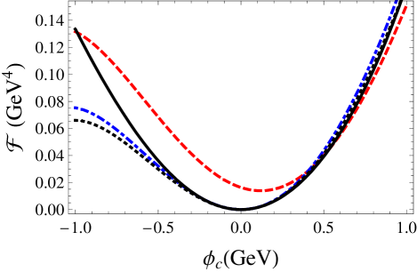
Figure 1: (color online) The free energy, in the $\phi_{c}$ direction, as a function of the classical field for $\Lambda_{{\overline{\rm MS}}}=0.9\,{\rm GeV}$, $M=1\,{\rm GeV}$, $m_{s}=0.55\,{\rm GeV}$, and $g_{s}=1$. The dashed line is the $\overline{\rm MS}$ renormalization scheme result. The dotted-dashed corresponds to $\Gamma^{(0)}=\Gamma^{(1)}=0$ while $\overline{\rm MS}$ is used in the remaining three 1PI function. The same situation but with $\Gamma^{(2)}=0$ is represented by the dotted line. The continuous line represents the LHA prescription.

If instead, like Chin, one adopts the so-called on-mass renormalization scheme the counterterms completely eliminate the total contributions represented by Eqs (13-17). Within this choice the results are scale independent while $M$, $m_{s}$, and $m_{v}$ represent the measurable physical masses at zero density whereas the three and four-body mesonic couplings vanish in agreement with the tree level result displayed by the original lagrangian density. The free energy generated by this scheme is represented by the dashed line in Fig. 2. Considering the relevant $K_{F}=0$ case, let us find a hybrid alternative scheme between the ${\overline{\rm MS}}$ and the on-mass-shell so that a residual, scale dependent, contribution survives within the three and four 1PI Green’s function given by Eqs (16) and (17).

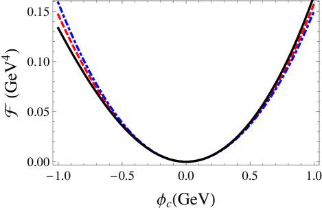
Figure 2: (color online) The free energy, in the $\phi_{c}$ direction, as a function of the classical field for $\Lambda_{{\overline{\rm MS}}}=0.9\,{\rm GeV}$, $M=1\,{\rm GeV}$, $m_{s}=0.55\,{\rm GeV}$, and $g_{s}=1$. All curves represent the LHA prescription at the different scales $\Lambda_{{\overline{\rm MS}}}=0.9\,{\rm GeV}<M$ (continuous line), $\Lambda_{{\overline{\rm MS}}}=1\,{\rm GeV}=M$ (dashed line) and $\Lambda_{{\overline{\rm MS}}}=1.1\,{\rm GeV}>M$. The dashed line also corresponds to the RHA result.

To do that, let us analyze each of the arbitrary $f_{n}$ terms contained in the counterterm coefficients from the physical point of view starting with $f_{0}$ which is contained in the field independent $\Gamma^{(0)}$. This contribution is renormalized by the constant counterterm $\alpha_{0}$ which can be referred to as the “cosmological constant” lowell . In practice, the only effect this term has is to give the zero point energy value and by its complete elimination one assures that ${\cal F}(\phi_{c}=0)=0$ which, within the Walecka model, will later assure that the pressure as well as the energy density vanish at $k_{F}=0$. Therefore, as in the on-mass shell prescription, we can impose that $f_{0}$ be exactly equal to the finite part of the $\Gamma^{(0)}$ term. It is important to point out that even if one uses the ${\overline{\rm MS}}$ scheme this term can be absorbed in a vacuum expectation value subtraction of the zero point energy so that the exact way in which it done is not too relevant for the present purposes.

The effect of the the linear (tadpole) term $\Gamma^{(1)}\phi_{c}$ is to shift the origin so that the minimum is not at the origin (${\bar{\phi}}_{c}\neq 0$) as shown by the dashed line of Fig. 1. Also any finite contribution left in the tadpole will cause direct terms to contribute to the baryon self energy which, at the present level of approximation, means that $M$ does not represent the physical nucleon mass at $k_{F}=0$, $M^{*}_{\rm vac}$. This can be understood by recalling that the baryon self-energy is $\Sigma_{B}\sim(g_{s}/m_{s}^{2}){\tilde{\Gamma}}^{(1)}(\Lambda_{{\overline{\rm MS}}})$ so that the vacuum effective baryon mass is given by $M^{*}_{\rm vac}=M+\Sigma_{B}(\Lambda_{{\overline{\rm MS}}})$ and since $M_{\rm sat}^{*}=939\,{\rm MeV}$ one sees that $M$, as well as $g_{s}$ and $m_{s}$, should depend on $\Lambda_{{\overline{\rm MS}}}$. However, for the purposes of controlling $K$ and $M_{\rm sat}^{*}$ the renormalization of the baryonic vacuum mass from $M$ to $M^{*}_{\rm vac}$ does not generate the wanted $\phi^{3}$ and $\phi^{4}$ vertices. Therefore, for simplicity, we can also set $f_{1}$ so as to completely eliminate the tadpole vacuum contribution. This choice for $f_{0}$ and $f_{1}$ together with $f_{2}=f_{3}=f_{4}=0$ produces the dot-dashed line of figure 1. The term $\Gamma^{(2)}$ represents a (momentum independent) vacuum correction to the scalar meson mass, $m_{s}$. As in the previous case, getting rid of this term assures that $m_{s}$ be taken as the physical mass simplifying the calculations since $(m_{s,{\rm vac}}^{*})^{2}=m_{s}^{2}+\Sigma_{s}(\Lambda_{{\overline{\rm MS}}})$ where $\Sigma_{s}(\Lambda_{{\overline{\rm MS}}})\sim{\tilde{\Gamma}}^{(2)}(\Lambda_{{\overline{\rm MS}}})$. Fixing $f_{2}$ so as to completely eliminate the $\Gamma^{(2)}$ contribution produces the dotted line of figure 1. In summary, so far we have adopted the usual Chin-Walecka on-mass shell renormalization conditions for $f_{1},f_{2}$, and $f_{3}$ so that: the vacuum energy is normalized to zero, $\phi_{c}=0$ is the minimum of $\cal F$ (also meaning that $M=M^{*}_{\rm vac}$), while $m_{s}$ represents the vacuum scalar meson mass. In this approach, none of the vacuum mass parameters present in the original lagrangian density run with $\Lambda_{{\overline{\rm MS}}}$. Note that, physically, our choice was also inspired by the NLWM observation that the compressibility modulus is improved by the introduction of $\phi^{3}$ and $\phi^{4}$ terms which is consistent with our choice of neglecting any corrections to terms proportional to $\phi{\bar{\psi}}\psi$ and $\phi^{2}$ which are directly related with the scalar meson and baryon masses.

Now, taking $f_{3}=0$ and $f_{4}=0$ would leave us with the wanted $\phi^{3}$ and $\phi^{4}$ scale dependent terms. However, inspection of Eq. (16) and Eq. (17) shows that these contributions would vanish at different scales, given by $\Lambda_{{\overline{\rm MS}}}=Me^{1/3}$ and $\Lambda_{{\overline{\rm MS}}}=Me^{4/3}$ respectively. As already emphasized the NLWM controls the compression modulus with the $\kappa\phi^{3}$ and $\lambda\phi^{4}$ terms so one can impose that, within our approach, both $\kappa_{\rm eff}$ and $\lambda_{\rm eff}$ arise at the same energy scale. This can be achieved by imposing that $\Gamma^{(3)}=\Gamma^{(4)}=0$ at $\Lambda_{{\overline{\rm MS}}}=M$ in which case the RHA is always reproduced. Finally, in our RG-NLWM inspired prescription we also impose that any $\Lambda_{{\overline{\rm MS}}}$ dependence should be left within the leading logs which naturally emerge within DR, as shown by Eqs (13-17), and which are the main contributing terms to the $\beta$ function. In this case, the $\alpha_{3}$ and $\alpha_{4}$ counterterms also eliminate the $\Lambda_{{\overline{\rm MS}}}$ independent constants in Eqs (16) and (17). One then obtains the continuous line of Fig. 1. The complete finite, scale dependent, vacuum contribution is then given by

$$\Delta_{R}^{\rm LHA}(\phi_{c},\Lambda_{\overline{\rm MS}}) = -\frac{\gamma}{16\pi^{2}}\left[(M-g_{s}\phi_{c})^{4}\,\ln\left(\dfrac{M-g_{s}\phi_{c}}{M}\right)+g_{s}\phi_{c}M^{3}-\frac{7}{2}(g_{s}\phi_{c})^{2}M^{2}+\frac{13}{3}(g_{s}\phi_{c})^{3}M-\frac{25}{12}(g_{s}\phi_{c})^{4}\right]$$ (20)

$$+ \frac{\gamma}{4\pi^{2}}\left[(g_{s}\phi_{c})^{3}M-\frac{1}{4}(g_{s}\phi_{c})^{4}\right]\ln\left(\frac{M}{\Lambda_{{\overline{\rm MS}}}}\right)\,.$$

The free energy obtained with this finite vacuum contribution term is shown in Fig 2 for $\Lambda_{{\overline{\rm MS}}}<M$ (continuous line), $\Lambda_{{\overline{\rm MS}}}>M$ (dot-dashed line) as well as for $\Lambda_{{\overline{\rm MS}}}=M$ (dashed line) in which case the usual RHA is retrieved. As one can check, the first term in Eq. (20) is just the RHA vacuum correction chin so that, in view of Eq. (2), one can write

$$\Delta_{R}^{\rm LHA}(\phi_{c},\Lambda_{\overline{\rm MS}})=\Delta_{R}^{\rm RHA}(\phi_{c})+\frac{\kappa_{\rm eff}}{3!}\phi_{c}^{3}+\frac{\lambda_{\rm eff}}{4!}\phi_{c}^{4}\,\,\,,$$ (21)

where $\kappa_{\rm eff}=2g_{s}^{3}Mb_{\rm eff}(\Lambda_{\overline{\rm MS}})$ and $\lambda_{\rm eff}=6g_{s}^{4}c_{\rm eff}(\Lambda_{\overline{\rm MS}})$ with

$$b_{\rm eff}(\Lambda_{\overline{\rm MS}})=\frac{3}{\pi^{2}}\ln\left(\frac{M}{\Lambda_{{\overline{\rm MS}}}}\right)$$ (22)

and $b_{\rm eff}(\Lambda_{\overline{\rm MS}})=-3\,c_{\rm eff}(\Lambda_{\overline{\rm MS}})$. In this way not only $\kappa_{\rm eff}$ and $\lambda_{\rm eff}$ vanish at the same scale but an inversion of their respective signs happen at the same time. We have then achieved our goal by quanticaly inducing $\kappa=0\to\kappa_{\rm eff}(\Lambda_{\overline{\rm MS}})$ and $\lambda=0\to\lambda_{\rm eff}(\Lambda_{\overline{\rm MS}})$ in a way that all the scale dependence is contained in the leading logs and also achieving $\kappa_{\rm eff}(\Lambda_{\overline{\rm MS}})=\lambda_{\rm eff}(\Lambda_{\overline{\rm MS}})=0$ at $\Lambda_{\overline{\rm MS}}=M$.

For comparison purposes let us quote the MRHA result

$$\Delta_{R}^{\rm MRHA}(\phi_{c},\Lambda)=\Delta_{R}^{\rm RHA}(\phi_{c})+\gamma\frac{(g_{s}\phi_{c})^{3}}{4\pi^{2}}\left[\ln\left(\frac{M}{\Lambda}\right)-1+\frac{\Lambda}{M}\right]-\gamma\frac{(g_{s}\phi_{c})^{4}}{16\pi^{2}}\ln\left(\frac{M}{\Lambda}\right)\,\,.$$ (23)

One notices that the major difference between the MRHA and our prescription amounts to the finite contribution contained within the cubic term where the scale dependence is not restricted to the leading log being also contained in an extra linear term which does not naturally arise when expands the DR results for the loop integrals in powers of $\epsilon$, as shown by Eqs. (13-17).

IV Renormalized Energy Density

To obtain the thermodynamical potential, $\Omega$, one minimizes the free energy (or effective potential) with respect to the fields. That is, $\Omega={\cal F}({\bar{\sigma}}_{c},{\bar{V}}_{0})=-P$, where $P$ represents the pressure. Then, the LHA renormalized pressure is

$$P^{\rm LHA}=\frac{m_{v}^{2}}{2}{\overline{V}}_{c,0}^{2}-\frac{m_{s}^{2}}{2}{\bar{\phi}}_{c}^{2}+\gamma\int_{0}^{k_{F}}\frac{d^{3}{\bf k}}{(2\pi)^{3}}\left[(\mu-g_{v}{\overline{V}}_{0,c})-E^{*}({\bf k})\right]-\Delta_{R}^{\rm LHA}({\bar{\phi}}_{c},\Lambda_{\overline{\rm MS}})$$ (24)

where $E^{*}=({\bf k}^{2}+M^{*})^{1/2}$ with $M^{*}=M-g_{s}{\bar{\phi}}_{c}$ while the Fermi momentum is given by $k_{F}^{2}=(\mu-g_{v}{\bar{V}}_{0,c})^{2}-{M^{*}}^{2}$. For the vector field one gets

$${\overline{V}}_{0,c}=\frac{g_{v}}{m_{v}^{2}}\rho_{B}\,\,,$$ (25)

where $\rho_{B}=(\gamma k_{F}^{3})/(6\pi^{2})$ is the baryonic density whereas for the scalar field the result is

$${\bar{\phi}}_{c}=\frac{g_{s}}{m_{s}^{2}}[\rho_{s}+\Delta^{\prime\,{\rm LHA}}_{R}({\bar{\phi}}_{c})]\,\,\,,$$ (26)

where

$$\rho_{s}=\gamma\frac{M^{*}}{2\pi^{2}}\int_{0}^{k_{F}}d{\bf k}\frac{{\bf k}^{2}}{E^{*}({\bf k})}\;,$$ (27)

represents the scalar density and

$$\Delta^{\prime\,{\rm LHA}}_{R}({\bar{\phi}}_{c}) = -\frac{\gamma}{4\pi^{2}}\left[{M^{*}}^{3}\ln\left(\frac{M^{*}}{M}\right)+g_{s}{\bar{\phi}}_{c}M^{2}-\frac{5}{2}(g_{s}{\bar{\phi}}_{c})^{2}M+\frac{11}{6}(g_{s}{\bar{\phi}}_{c})^{3}\right]$$ (28)

$$+ \frac{\gamma}{4\pi^{2}}\left[3(g_{s}{\bar{\phi}}_{c})^{2}M-(g_{s}{\bar{\phi}}_{c})^{3}\right]\ln\left(\frac{M}{\Lambda_{{\overline{\rm MS}}}}\right)\;.$$

To get the energy density, $\cal E$, one can use the relation ${\cal E}=-P+\mu\rho_{B}$ obtaining

$${\cal E}^{\rm LHA}=\frac{g_{v}^{2}}{2m_{v}^{2}}\rho_{B}^{2}+\frac{m_{s}^{2}}{2}{\bar{\phi}}_{c}^{2}+\frac{\gamma}{2\pi^{2}}\int_{0}^{k_{F}}{\bf k}^{2}d{\bf k}E^{*}({\bf k})+\Delta_{R}^{\rm LHA}(M^{*},\Lambda_{\overline{\rm MS}})\;,$$ (29)

where

$$\Delta_{R}^{\rm LHA}(M^{*},\Lambda_{\overline{\rm MS}}) = -\frac{\gamma}{16\pi^{2}}\left[{M^{*}}^{4}\,\ln\left(\dfrac{M^{*}}{M}\right)+(M-M^{*})M^{3}-\frac{7}{2}(M-M^{*})^{2}M^{2}\right.$$ (30)

$$+ \left.\frac{13}{3}(M-M^{*})^{3}M-\frac{25}{12}(M-M^{*})^{4}\right]$$

$$+ \dfrac{\gamma}{4\pi^{2}}\left[(M-M^{*})^{3}M-\frac{1}{4}(M-M^{*})^{4}\right]\ln\left(\dfrac{M}{\Lambda_{{\overline{\rm MS}}}}\right)\;,$$

and

$$M^{*}=M-\gamma\frac{g_{s}^{2}}{m_{s}^{2}}\frac{M^{*}}{2\pi^{2}}\int_{0}^{k_{F}}\frac{{\bf k}^{2}}{E^{*}({\bf k})}d{\bf k}-\frac{g_{s}^{2}}{m_{s}^{2}}\Delta_{R}^{\prime}(M^{*},\Lambda_{\overline{\rm MS}})\;,$$ (31)

where

$$\Delta^{\prime\,{\rm LHA}}_{R}(M^{*},\Lambda_{\overline{\rm MS}}) = -\frac{\gamma}{4\pi^{2}}\left[{M^{*}}^{3}\ln\left(\frac{M^{*}}{M}\right)+(M-M^{*})M^{2}-\frac{5}{2}(M-M^{*})^{2}M+\frac{11}{6}(M-M^{*})^{3}\right]$$ (32)

$$+ \frac{\gamma}{4\pi^{2}}\left[3(M-M^{*})^{2}M-(M-M^{*})^{3}\right]\ln\left(\frac{M}{\Lambda_{{\overline{\rm MS}}}}\right)\;.$$

V Numerical Results

Let us now investigate the numerical results furnished by LHA for the baryon mass at saturation as well as for the compressibility modulus, with the latter given by

$$K=\left[k^{2}\frac{\partial^{2}}{\partial k^{2}}\left(\frac{\varepsilon}{\rho_{B}}\right)\right]_{k=k_{F}}=9\left[\rho_{B}^{2}\frac{\partial^{2}}{\partial\rho_{B}^{2}}\left(\frac{\varepsilon}{\rho_{B}}\right)\right]_{\rho_{B}=\rho_{0}}\;.$$ (33)

Table 1 shows the coupling constants and saturation properties for some values of the renormalization scale ($\Lambda_{\overline{\rm MS}}$) that yield $BE=-15.75$ MeV and $k_{F}=1.42$ fm^-1 (280.20 MeV). These values are chosen just in order to compare with the original Walecka Model (QHD-I) waleckaANP . The meson masses are $m_{s}=512$ MeV and $m_{v}=783$ MeV. This table shows that some of the best LHA values are obtained with $\Lambda_{\overline{\rm MS}}$ values which are very close to $M$. Since at $\Lambda_{\overline{\rm MS}}=M$ the RHA result is reproduced one concludes, based on our results, that slight decrease from the RHA energy scale produces an enormous effect on the values of both, $K$ and $M^{*}_{\rm sat}$.

Table 1: Coupling constants and saturation properties for some values of the renormalization scale ($\Lambda_{\overline{\rm MS}}$) that yield $BE=-15.75$ (MeV) and $k_{F}=1.42$ fm^-1. The meson masses are $m_{s}=512$ MeV and $m_{v}=783$ MeV.

	$\Lambda_{\overline{\rm MS}}/M$	$K$ (MeV)	$M^{*}_{\rm sat}/M$	$C_{v}^{2}$	$C_{s}^{2}$	$g_{v}^{2}$	$g_{s}^{2}$	$\kappa_{\rm eff}/M$	$\lambda_{\rm eff}$
($\overline{\rm MS}$)	1.030	1279.408	0.606	171.339	176.984	119.138	52.619	-6.859	49.753
($\overline{\rm MS}$)	1.020	910.234	0.646	151.744	184.093	105.512	54.736	-4.875	36.063
($\overline{\rm MS}$)	1.010	639.833	0.684	132.232	185.875	91.945	55.263	-2.485	18.474
($\overline{\rm MS}$)	1.005	542.279	0.702	123.626	185.609	85.961	55.184	-1.243	9.233
($\overline{\rm MS}$)	1.000	468.140	0.718	114.740	183.300	79.782	54.497	0.000	0.000
($\overline{\rm MS}$)	0.990	371.437	0.745	99.784	177.933	69.383	52.901	2.351	-17.099
($\overline{\rm MS}$)	0.980	314.086	0.767	88.623	173.525	61.622	51.591	4.551	-32.689
($\overline{\rm MS}$)	0.975	294.260	0.776	84.456	172.456	58.725	51.273	5.651	-40.463
($\overline{\rm MS}$)	0.970	277.989	0.784	80.307	170.683	55.840	50.746	6.694	-47.684
($\overline{\rm MS}$)	0.960	253.249	0.798	73.691	168.648	51.240	50.141	8.811	-62.391
($\overline{\rm MS}$)	0.950	235.660	0.809	67.923	166.440	47.229	49.484	10.855	-76.356
($\overline{\rm MS}$)	0.940	222.493	0.818	63.025	164.576	43.824	48.930	12.875	-90.058
($\overline{\rm MS}$)	0.920	202.507	0.832	55.411	162.702	38.529	48.373	17.054	-118.611
($\overline{\rm MS}$)	0.900	188.175	0.843	49.467	161.826	34.396	48.112	21.375	-148.267
($\overline{\rm MS}$)	0.8595	166.351	0.8595	40.936	164.038	28.464	48.770	31.349	-218.926
($\overline{\rm MS}$)	0.850	162.638	0.863	39.348	165.080	27.360	49.080	33.971	-237.992
($\overline{\rm MS}$)	0.800	144.532	0.876	32.511	172.680	22.606	51.340	49.902	-357.552
($\overline{\rm MS}$)	0.700	118.409	0.893	23.328	200.551	16.221	59.626	99.833	-770.891
($\overline{\rm MS}$)	0.600	98.285	0.905	17.052	256.570	11.857	76.281	206.893	-1806.98
($\overline{\rm MS}$)	0.500	81.019	0.914	12.239	397.387	8.510	118.147	541.142	-5881.97
($\overline{\rm MS}$)	0.400	65.319	0.921	8.235	1290.240	5.726	383.600	4185.070	-81967.5
(RHA)	-	468.140	0.718	114.740	183.300	79.782	54.497	-	-
(MFT)	-	546.610	0.556	195.900	267.100	136.210	79.423	-	-

Figures 3 (a) and (b) show the binding energy per baryon, $BE=E/A-M$, and the effective baryon mass as functions of the Fermi momentum for some $\Lambda_{\overline{\rm MS}}$ values, shown in table 1. One easily sees the effect of considering the vacuum contribution and its improvements on the compressibility and the effective mass. As expected, when $\Lambda_{\overline{\rm MS}}=M$, the RHA results are recovered. From figures 4 (a) and (b) it is possible to see some properties obtained in table 1 within the LHA approach, as functions of $\Lambda_{\overline{\rm MS}}/M$. One notes from figure 4 (a) that when $\Lambda_{\overline{\rm MS}}$ increases the value of the nuclear compressibility ($K$) also increases and $M^{*}_{\rm sat}$ decreases. The crossing point in figure 4 (a) represents the RHA values of $K$ and $M^{*}$ which occurs when we set $\Lambda_{\overline{\rm MS}}=M$. Figure 4 (b) shows the effective couplings that arise due to the LHA as functions of $\Lambda_{\overline{\rm MS}}/M$. Similarly when $\Lambda_{\overline{\rm MS}}$ reaches the value $M$ the RHA results are recovered and the effective couplings vanish.

(a)	(b)

Figure 3: (a) Binding energy per nucleon as a function of the Fermi momentum for different values of our scale $\Lambda_{\overline{\rm MS}}$. We also plot the MFT and RHA results for comparison purposes. The saturation properties are: $BE=-15.75$ MeV and $k_{F}=1.42$ fm^-1 (280.20 MeV). (b) Similar as figure (a) but for the effective baryon mass $M^{*}$ as a function of the Fermi momentum for different values of the scale. Note that when $\Lambda_{\overline{\rm MS}}=1$ we reproduce the RHA results.

(a)	(b)

Figure 4: Some properties obtained in table 1 within the LHA approach, as a function of the renormalization scale $\Lambda_{\overline{\rm MS}}$ in units of the baryon mass. (a) Compression modulus and effective baryon mass $\times$ $\Lambda_{\overline{\rm MS}}/M$ and (b) effective couplings that arise due to the LHA as functions of $\Lambda_{\overline{\rm MS}}/M$. They vanish when $\Lambda_{\overline{\rm MS}}/M=1$ and the RHA results are reproduced as one sees in table 1.

To compare our numerical results with those provided by the MRHA let us make a remark concerning the effective nucleon mass. From a non-relativistic analysis of scattering of neutron-Pb nuclei it has been found johnsonHoren that $M_{\rm sat}^{*}/M\approx 0.74~{}{\rm to}~{}0.82$ which can be viewed as approximately describing the Landau effective mass glenM . The relativistic isoscalar component known as the effective mass defined in Eq. (31) can be called the Dirac effective mass and is related to the Landau effective mass. Therefore, the range expected for the Dirac effective mass at saturation density lies in the range $M_{\rm sat}^{*}/M\approx 0.70~{}{\rm to}~{}0.80$ whereas for the nuclear compressibility at saturation the most widely accepted values are $K\approx 200\,{\rm MEV}~{}{\rm to}~{}300$ MeV blaizotK . For this range of $K$ and according to table 2 the MRHA predicts $M_{\rm sat}^{*}/M\approx 0.80~{}{\rm to}~{}0.85$ for $\Lambda/M\approx 1.185~{}{\rm to}~{}1.466$. However, one should note that this MRHA energy scale range is not unique and can also be reproduced with $\Lambda/M\approx 0.753~{}{\rm to}~{}0.778$ which in turn leads to a rather low range for $M_{\rm sat}^{*}$ values, $M_{\rm sat}^{*}/M\approx 0.65~{}{\rm to}~{}0.69$. Our results, shown in tables 1 and 2, seem to produce a better agreement for this range of $K$ giving the unique range $M_{\rm sat}^{*}/M\approx 0.76~{}{\rm to}~{}0.83$ for $\Lambda_{\overline{\rm MS}}/M\approx 0.920~{}{\rm to}~{}0.977$ with $\kappa_{\rm eff}>0$ and $\lambda_{\rm eff}<0$.

As a last remark we would like to point out that if one chooses $\Lambda_{\overline{\rm MS}}/M=0.9805$, $(g_{s}/m_{s})^{2}=9.468$ fm² and $(g_{v}/m_{v})^{2}=4.879$ fm² the LHA approach reproduces the same saturation properties as performed by the so-called GM2 parameter set according to glenGM123 : $K=300$ MeV, $M_{\rm sat}^{*}/M=0.78$, $BE=-16.3$ MeV, $k_{F}=1.313$ fm^-1 and $\rho_{0}=0.153$ fm^-3. The resulting effective couplings are: $b_{\rm eff}=0.005986$ and $c_{\rm eff}=-0.001995$.

Table 2: Comparison between the LHA and the MRHA approaches with other estimates.

	$\Lambda_{s}/M$	$K$ (MeV)	$M^{*}/M$
MRHA rudaz	1.185 - 1.466	300 - 200	0.80 - 0.85
MRHA rudaz	0.778 - 0.753	300 - 200	0.65 - 0.69
LHA	0.977 - 0.920	300 - 200	0.76 - 0.83
Estimates johnsonHoren ; glenM ; blaizotK	-	300 - 200	0.70 - 0.80
Where $\Lambda_{s}=\Lambda$ for MRHA and LHA is given by: $\Lambda_{s}=\Lambda_{\overline{\rm MS}}$ .

In the appendix we show that leaving a leading log dependence also in the two point Green’s function, $\Gamma^{(2)}$, only increases the numerical complexity without producing results better than the ones generated by the simplest LHA version employed so far.

VI Conclusions

We considered the simplest form of the Walecka model to analyze how the values of the compressibility modulus as well as the baryon mass, at saturation, can be improved by adopting an appropriate renormalization scheme in which cubic and quartic effective couplings are radiatively generated. With this aim we have evaluated the effective potential to the one loop level using Matsubara’s formalism to introduce the density dependence. The vacuum contributions have been evaluated using dimensional renormalization compatible with the ${\overline{\rm MS}}$ renormalization scheme.

We have then chosen the renormalization conditions in such a way so that all the mass parameters appearing in the original lagrangian density represent the physical mass at zero density and therefore do not run with the energy scale. For our purposes the most important part was to renormalize the values of the cubic and quartic terms ($\kappa\phi^{3}/3!$ and $\lambda\phi^{4}/4!$) which vanish at the classical (tree) level in the original model. We have then allowed only scale dependent logarithms, which naturally arise within DR, to be present in the final finite expressions and, contrary to the MRHA prescription, we obtained that both couplings have exactly the same type of scale dependence. In other words, the parameters $b$ and $c$ contained in the cubic and quartic terms have been dressed by one loop vacuum contributions so that $b=0\to b_{\rm eff}=3/\pi^{2}\ln(\Lambda_{\overline{\rm MS}}/M)$ and $c=0\to-b_{\rm eff}/3$.

In our approach each value of the energy scale produces only one value for $K$ and $M_{\rm sat}^{*}$ while two values can be obtained within the MRHA. In our case the best values for these physical quantities occur at energy scales very close to the highest mass value, $M$. Since the RHA is obtained for $\Lambda_{\overline{\rm MS}}=M$ one concludes that a small variation around this value of the energy scale can significantly improve both $K$ and $M_{\rm sat}^{*}$ as shown by our numerical results which predict $M_{\rm sat}^{*}/M\approx 0.76~{}{\rm to}~{}0.83$ and $K\approx 200\,{\rm MeV}~{}{\rm to}~{}300$ MeV at $\Lambda_{\overline{\rm MS}}/M\approx 0.920~{}{\rm to}~{}0.977$. These results turn to be in excellent agreement with the most quoted estimates $M_{\rm sat}^{*}/M\approx 0.70~{}{\rm to}~{}0.80$ and $K\approx 200\,{\rm MeV}~{}{\rm to}~{}300$ MeV. To achieve these $K$ values the MRHA predicts either $M_{\rm sat}^{*}/M\approx 0.80~{}{\rm to}~{}0.85$ or $M_{\rm sat}^{*}/M\approx 0.65~{}{\rm to}~{}0.69$ in the two possible energy scale ranges. Recalling that at $\Lambda_{\overline{\rm MS}}/M=1$ the (RHA) results are $M_{\rm sat}^{*}/M=0.718$ and $K=468.14\,{\rm MeV}$ one may further appreciate how a small tuning of the energy scale within the LHA greatly improves the situation. To compare the LHA with the MRHA we recall that the philosophy within the latter is that many-body effects in nuclear matter at saturation can be minimized by choosing the energy scale close to $M^{*}_{\rm sat}$ in which case the values $M^{*}_{\rm sat}/M=0.731$ and $K=162\,{\rm MeV}$ are reproduced. Although the former seems reasonable the latter seems too low according to the above quoted estimates. The philosophy of the LHA, proposed in the present work, is to keep only the scale dependent leading logs in the finite parts of the effective cubic and quartic couplings.

In practice, the main difference between the two approximations is reflected by the fact that the MRHA effective cubic coupling, apart from the logarithmic term, also displays a term which depends linearly on the energy scale accounting for the numerical differences cited above. It is worth pointing out that, within the LHA as well as the MRHA, a given scale sets both $\kappa_{\rm eff}$ and $\lambda_{\rm eff}$ so that both $K$ and $M_{\rm sat}^{*}$ cannot be separately tuned as in the NLWM where $\kappa$ and $\lambda$ can be set separately. However, even in an effective theory such as the Walecka model, an increase in the parameter space as the one generated by the NLWM can be viewed as an unwanted feature and the LHA succeeds in improving the values of $K$ of $M_{\rm sat}^{*}$ without the drawback of increasing many body effects and parameter space. The method proposed here should be easy to be implemented within many existing MFA or RHA applications where $\Delta^{\rm LHA}$ can be added to the energy density (in the MFA case) or used to replace the existing $\Delta^{\rm RHA}$ in a RHA type of calculation.

In principle the LHA philosophy could be extended to the two loop level in a calculation similar to the one performed in Refs. furnstahl1 and ijmpe . Then by tuning the energy scale appropriately one could try to reduce the size of the two loop corrections producing physically meaningful results.

Our method can be extended to applications related to neutron stars and evaluation of other physical quantities, such as the symmetry energy. In particular, models and/or approximations which lead to low effective masses at saturation are not suitable for neutron stars calculations since as the density increases the effective mass vanishes so quickly that higher densities cannot be properly reached as needed alex-debora . In principle, the LHA has potential to correct this problem without the need to introduce extra mesonic interactions with their respective parameters.

*

Appendix A

For completeness, let us check numerically the effects of leaving a leading log dependence also in the two point Green’s function with zero external momentum, $\Gamma^{(2)}$, given by Eq. (15). Then,

$$\Delta^{{\rm LHA}}_{R}(M^{*},\Lambda_{\overline{\rm MS}})\to\Delta^{{\rm LHA}}_{R}(M^{*},\Lambda_{\overline{\rm MS}})-(M-M^{*})^{2}M^{2}\frac{\gamma}{16\pi^{2}}\left[6\ln\left(\frac{M}{\Lambda_{{\overline{\rm MS}}}}\right)\right]\;,$$ (34)

and

$$\Delta^{\prime\,{\rm LHA}}_{R}(M^{*},\Lambda_{\overline{\rm MS}})\to\Delta^{\prime\,{\rm LHA}}_{R}(M^{*},\Lambda_{\overline{\rm MS}})-(M-M^{*})M^{2}\frac{\gamma}{8\pi^{2}}\left[6\ln\left(\frac{M}{\Lambda_{{\overline{\rm MS}}}}\right)\right]\;.$$ (35)

In this case, the effective potential gives a first (momentum independent) correction to the effective scalar mass in the vacuum is $m_{s,\rm vac}^{*}$. Then, for each energy scale, apart from the $BE$ requirement one also has to fix the parameter set so that the effective scalar meson mass, in the vacuum $m_{s,\rm vac}^{*}=512\,{\rm MeV}$. This effective mass is obtained by considering one loop momentum independent self energy

$$(m_{s,\rm vac}^{*})^{2}=m_{s}^{2}-M^{2}g_{s}^{2}\frac{\gamma}{8\pi^{2}}\left[6\ln\left(\frac{M}{\Lambda_{{\overline{\rm MS}}}}\right)\right]\,\,,$$ (36)

which clearly indicates that $m_{s}$ (as well as $g_{s}$) must run with the energy scale. However, this more cumbersome approach has almost no effect in our best results for $K$ and $M_{\rm sat}^{*}$ as table 3 shows indicating the adequacy of the LHA simple prescription previously adopted.

Table 3: Same as in table 1 for the case in which $\Gamma^{(2)}$ has a non vanishing leading log and $m_{s}$ runs with the energy scale.

	$\Lambda_{\overline{\rm MS}}/M$	$K$ (MeV)	$M_{\rm sat}^{*}/M$	$C_{v}^{2}$	$C_{s}^{2}$	$g_{v}^{2}$	$g_{s}^{2}$	$m_{s}$ (MeV)
($\overline{\rm MS}$)	1.000	468.140	0.718	114.740	183.300	79.782	54.497	512.000
($\overline{\rm MS}$)	0.975	294.260	0.776	84.456	74.106	58.725	22.032	641.594
($\overline{\rm MS}$)	0.950	235.660	0.809	67.923	46.297	47.229	13.765	671.839
($\overline{\rm MS}$)	0.920	202.507	0.832	55.411	31.755	38.529	9.441	687.840

References

- (1) J. D. Walecka, Ann. Phys. (N.Y.) 83, 491 (1974); B. D. Serot and J.D. Walecka, Adv. Nucl. Phys. 16 (1986);
- (2) P. Ramond, “Field Theory: a Modern Primer” (Westview Press, 2001); D. Bailin and A. Love, “Introduction to Gauge Field Theory Revised Edition” (Taylor and Francis, 1993).
- (3) S. A. Chin, Phys. Lett. B62, 263 (1976); Ann. Phys. (N.Y.) 108, 301 (1977).
- (4) R. J. Furnstahl, R. J. Perry and B. D. Serot, Phys. Rev. C 40, 321 (1989); Erratum Phys. Rev. C 42, 2040 (1990).
- (5) A Bielajew and B. Serot, Ann. Phys. (N.Y.) 156, 215 (1984).
- (6) D. P. Menezes, M. B. Pinto and D. P. Menezes, Int. J. of Mod. Phys. E 9, 221 (2000).
- (7) J. Boguta and A. R. Bodmer, Nucl. Phys. A292, 413 (1977).
- (8) E. K. Heide and S. Rudaz, Phys. Lett. B262, 375 (1991).
- (9) M. Prakash, P. J. Ellis, E. K. Heidi and S. Rudaz, Nucl.Phys A575, 583 (1994); S. S. Rocha, A. R. Taurines, C. A. Z. Vaconcellos, M. B. Pinto, and M. Dillig, Mod. Phys. Lett. A 17, 1335 (2002).
- (10) W. Zisheng, M. Zhongyu and Z. Yizhong, Phys. Rev. C 55, 3159 (1997).
- (11) L. Brown, “Quantum Field Theory” (CUP, 1994).
- (12) C. H. Johnson, D. J. Horen and C. Mahaux, Phys. Rev. C 36, 2252 (1987); C. Mahaux and R. Sartor, Nucl. Phys. A475, 247 (1987); Nucl. Phys. A493, 157 (1989).
- (13) N. K. Glendenning, Phys. Rev. C 37, 2733 (1988); M. Jaminon and C. Mahaux, Phys. Rev. C 40, 354 (1989); Zhong-Yu Ma, Jian Rong, Bao-Qiu Chen, Zhi-Yuan Zhu and Hong-Qiu Song, Phys. Lett. B604, 170 (2004).
- (14) J. P. Blaizot, D. Gogny and B. Grammiticos, Nucl. Phys. A265, 315 (1976); J. P. Blaizot, Phys. Rep. 64, 171 (1980); H. Krivine, J. Treiner and O. Bohigas, Nucl. Phys. A336, 155 (1980); N. K. Glendenning, Phys. Rev. Lett. 57, 1120 (1986); Phys. Rev. C 37, 2733 (1988); M. M. Sharma, W. T. A. Borghols, S. Brandenburg, S. Crona, A. van der Woude and M. N. Harakeh, Phys. Rev. C 38, 2562 (1988).
- (15) N. K. Glendenning, Phys. Rev. Lett. 67, 2414 (1991).
- (16) A. M. S. Santos and D. P. Menezes, Phys. Rev. C 69, 045803 (2004); Braz. J. Phys. 34, 833 (2004).