Chapter 1 Extreme Eigenvalues of Wishart Matrices: Application to Entangled Bipartite System

Satya N. Majumdar
 
Laboratoire de Physique Théorique et Modèles Statistiques (UMR 8626 du CNRS) Université Paris-Sud, Bâtiment 100 91405 Orsay Cedex, France

Abstract

This chapter discusses an application of the random matrix theory in the context of estimating the bipartite entanglement of a quantum system. We discuss how the Wishart ensemble (the earliest studied random matrix ensemble) appears in this quantum problem. The eigenvalues of the reduced density matrix of one of the subsystems have similar statistical properties as those of the Wishart matrices, except that their trace is constrained to be unity. We focus here on the smallest eigenvalue which serves as an important measure of entanglement between the two subsystems. In the hard edge case (when the two subsystems have equal sizes) one can fully characterize the probability distribution of the minimum eigenvalue for real, complex and quaternion matrices of all sizes. In particular, we discuss the important finite size effect due to the fixed trace constraint.

1.1 Introduction

The different chapters of this book have already illustrated numerous applications of random matrices in a variety of problems ranging from physics to finance. In this chapter, I will demonstrate yet another beautiful application of random matrix theory in a bipartite quantum system that is entangled. Entanglement has off late become a rather fashionable subject due to its applications in quantum information theory and quantum computation. Entanglement serves as a simple measure of nonclassical correlations between different parts of a quantum system. The more the entanglement between two parts of a system, better it is for the functioning of algorithms of quantum computation. This is so because, intuitively speaking, quantum states that are highly entangled contain more informations about different subparts of the composite system. In this chapter I will discuss the statistical properties of the entanglement in a particularly simple model of the ‘random pure state’ of a bipartite system. We will see how random matrices come into play in such a system.

Indeed, historically the earliest studied ensemble of random matrices is the Wishart ensemble (introduced by Wishart [Wis28] in 1928 in the context of multivariate data analysis, much before Wigner introduced the standard Gaussian ensembles of random matrices in the physics literature). Wishart matrices have found wide applications in a variety of systems (see the discussion later and also chapter 28 and chapter 40 of this book). In this chapter, we will see that the Wishart ensemble ( with a fixed trace constraint) also appears quite naturally as the reduced density matrix of a coupled entangled bipartite quantum system. The plan of this chapter, after a brief introduction to Wishart matrices, is to explore this connection more deeply with a particular focus on the statistics of the minimum eigenvalue which serves as a useful measure of entanglement.

Let us start with a brief recollection of the Wishart matrices. Consider a square $(N\times N)$ matrix $W$ of the product form $W=XX^{\dagger}$ where $X$ is a $(N\times M)$ rectangular matrix with real, complex or quaternion entries and $X^{\dagger}$ its conjugate. The matrix $W$ has a simple and natural interpretation. For example, let the entries $X_{ij}$ of the $X$ matrix represent some data, e.g., the price of the $i$-th commodity on, say, the $j$-th day of observation. So, there are $N$ commodities and for each of them we have the prices for $M$ consecutive days, represented by the $(N\times M)$ array $X$. Thus for each commodity, we have $M$ different samples. The product $(N\times N)$ matrix $W=XX^{\dagger}$ then represents the (unnormalized) covariance matrix, i.e., the correlation matrix between the prices of $N$ commodities. If the entries of $X$ are independent Gassian random variables chosen from the joint distribution $P[\{X_{ij}\}]\propto\exp\left[-\frac{\beta}{2}{\rm Tr}(XX^{\dagger})\right]$ (where the Dyson index $\beta=1$, $2$, or $4$ corresponds respectively to real, complex or quaternion entries), then the random covariance matrix $W$ is called the Wishart matrix [Wis28]. This ensemble is also referred to as the Laguerre ensemble since its spectral properties involve Laguerre polynomials [Bro65, For93].

As mentioned earlier, since its introduction Wishart matrices have found an impressive list of applications. They play an important role in statistical data analysis [Wil62, Joh01], in particular in data compression techniques known as Prinicipal Component Analysis (PCA) (see chapter 28 and chapter 40 of this book) with applications in image processing [Fuk90], biological microarrays [Hol00, Alt00], population genetics [Pat06, Nov08], finance [Bou01, Bur04], meteorology and oceanography [Pre88] amongst others. In physics, Wishart matrices have appeared in multiple areas: in nuclear physics [Fyo97], in low energy QCD and gauge theories  [Ver94a] (see also chapter 32 of this book), quantum gravity [Amb94, Ake97] and also in several problems in statistical physics. These include directed polymers in a disordered medium [Joh00], nonintersecting Brownian excursions [Kat03, Sch08] and fluctuating nonintersecting interfaces over a solid substrate [Nad09]. Several deformations of Wishart ensemble, with multiple applications, have also been studied in the literature [Ake08].

The Wishart matrix $W$ has $N$ non-negative random eigenvalues denoted by $\{w_{1},w_{2},\ldots,w_{N}\}$ ($w_{i}\geq 0$ for each $i$) whose spectral properties are well understood and some of them will be briefly reviewed in section 1.2. These include the joint distribution of $N$ eigenvalues, the average density of eigenvalues and also the distribution of extreme eigenvalues (the largest and the smallest). In this chapter we will be mostly concerned with the distribution of the smallest eigenvalue $w_{\rm min}={\rm min}(w_{1},w_{2},\ldots,w_{N})$ in the particular case $M=N$ corresponding to the so called hard edge (at the origin) case where the average $\langle w_{\rm min}\rangle\to 0$ as $N\to\infty$. In this case, the properties of the small eigenvalues (near $w=0$) are governed by Bessel functions in the large $N$ limit [Ede88, For93, Nag93, Ver94b, Nag95]. Such hard edge properties are absent in the traditional Wigner-Dyson Gaussian random matrix [Meh04] whose eigenvalues can be both positive and negative.

The reason we are interested in the smallest eigenvalue distribution of the Wishart matrix is because of its application in the seemingly unrelated quantum entanglement problem which is the main objective of this chapter. As we will see later, Wishart matrices will appear naturally as the reduced density matrix in a coupled bipartite quantum system that is in an entangled random pure state. There is a slight twist though: the Wishart matrix in this system satisfies a constraint, namely its trace is fixed to unity. This fixed trace ensemble is thus analogus to the microcanonical ensemble in statistical mechanics while the standard (unconstrained) Wishart ensemble being the analogue of the canonical ensemble in statistical mechanics (for other discussions on fixed trace ensembles see chapter 14, section 14.3.2 of this book). In particular, our emphasis will be on the distribution of the smallest eigenvalue $\lambda_{\rm min}$ in this fixed trace Wishart ensemble. This is because the smallest eigenvalue turns to be a very useful observable in this system which contains informations about entanglement. For the special case $M=N$ (hard edge), we will see that the distribution of $\lambda_{\rm min}$ can be exactly computed for all $N$ in this fixed trace ensemble in all three cases $\beta=1$, $\beta=2$ and $\beta=4$. In particular, we will discuss how the fixed trace constraint modifies the distribution of $\lambda_{\rm min}$ from its counterpart in the canonical Wishart ensemble. We will see that the global fixed trace constraint gives rise to rather strong finite size effects. This is relevant in the quantum context where the subsystems can be just a few qubits. So, it is actually important to know the distribution of entanglement for finite size systems (the thermodynamic limit is not always relevant in this context). Hence, the fact that one can compute the distribution of the minimum eigenvalue exactly for all $N$ (not necessarily large) in presence of the fixed trace constraint becomes important and relevant.

This rest of the chapter is organized as follows. In section 1.2, we briefly review some spectral properties of unconstrained Wishart matrices. In section 1.3 we introduce the problem of the random pure state of an entangled quantum bipartite system. Its connection to Wishart matrices with a fixed trace constraint is established. Next we focus on the smallest eigenvalue and derive its probability distribution for the bipartite problem in section 1.4. Finally we conclude in section 1.5 with a summary and open problems.

1.2 Spectral Properties of Wishart Matrices: A brief summary

Let us first briefly recall some spectral properties of the $(N\times N)$ Wishart matrix $W=XX^{\dagger}$ with $X$ being a rectangular $(N\times M)$ matrix with real $(\beta=1)$, complex $(\beta=2)$ or quaternion $(\beta=4)$ Gaussian entries drawn from the joint distribution $P[\{X_{ij}\}]\propto\exp\left[-\frac{\beta}{2}{\rm Tr}(XX^{\dagger})\right]$. These results will be useful for the problem of the random pure state of the bipartite system to be discussed in the next section.

Joint distribution of eigenvalues: The $N$ eigenvalues of $W$, denoted by $\{w_{1},w_{2},\ldots,w_{N}\}$, are non-negative and have the joint probability density function (pdf) [Jam64]

$$P[\{w_{i}\}]=K_{N,M}\,e^{-\frac{\beta}{2}\sum_{i=1}^{N}w_{i}}\,\prod_{i=1}^{N}w_{i}^{\alpha\beta/2}\,\prod_{j<k}|w_{j}-w_{k}|^{\beta}$$ (1.2.1)

where $\alpha=(1+M-N)-2/\beta$ and the normalization constant $K_{N,M}$ can be computed exactly [Jam64]. Without any loss of generality, we will assume $N\leq M$. This is because if $N>M$, one can show that $N-M$ eigenvalues are exactly $0$ and the rest of the $M$ eigenvalues are distributed exactly as in Eq. (1.2.1) with $N$ and $M$ exchanged. Note that while for Wishart matrices $M-N$ is a non-negative integer and $\beta=1$, $2$ or $4$, the joint density in Eq. (1.2.1) is well defined for any $\beta>0$ and $\alpha>-2/\beta$ (this last condition is necessary so that the joint pdf is normalizable). When these parameters take continuous values the joint pdf is called the Laguerre ensemble.

Coulomb gas interpretation, typical scaling and average density of states: The joint pdf (1.2.1) can be written in the standard Boltzmann form, $P[\{w_{i}\}]\propto\exp\left[-\beta E(\{w_{i}\})\right]$ where

$$E[\{w_{i}\}=\frac{1}{2}\sum_{i=1}^{N}(w_{i}-\alpha\log w_{i})-\frac{1}{2}\sum_{j\neq k}\ln|w_{j}-w_{k}|$$ (1.2.2)

can be identified as the energy of a Coulomb gas of charges with positions $\{w_{i}\}\geq 0$. These charges repel each other via the $2$-d Coulomb (logarithmic) interaction (the second term in the energy), though they are restricted to live on the positive real line. In addition, these charges are subjected to an external potential which is linear+logarithmic (the first term in the energy ). The external potential tends to push the charges towards the origin while the Coulomb repulsion tends to spread them apart. The first term typically scales as $w_{\rm typ}N$ where $w_{\rm typ}$ is the typical value of an eigenvalue, while the second term scales as $N^{2}$ for large $N$. Balancing these two terms one gets $w_{\rm typ}\sim N$ for large $N$. Indeed, this scaling shows up in the average density of states (average charge density) which can be computed from the joint pdf and has the following scaling for large $N$

$$\rho_{N}(w)=\frac{1}{N}\sum_{i=1}^{N}\langle\delta(w-w_{i})\rangle\to\frac{1}{N}\,f_{\rm MP}\left(\frac{w}{N}\right)$$ (1.2.3)

where the Marcenko-Pastur(MP) scaling function is given by [Mar67] (see also chapter 28 section 28.4.1 of this book)

$$f_{\rm MP}(x)=\frac{1}{2\pi x}\,\sqrt{(b-x)(x-a)}.$$ (1.2.4)

Thus the charge density is confined over a finite support $[a,b]$ with the lower edge $a=(1-c^{-1/2})^{2}$ and the upper edge $b=(1+c^{-1/2})^{2}$ with $0\leq c=N/M\leq 1$. For all $c<1$, the average density vanishes at both edges of the MP sea. For the special case $c=1$ (this happens in the large $N$ limit when $M-N<<O(N)$), the lower edge $a$ gets pushed towards the hard wall at $0$ (this is the so called hard edge limit) and the upper edge $b\to 4$ and the average density simply becomes, $f_{\rm MP}(x)=\frac{1}{2\pi}\sqrt{(4-x)/x}$ for $0\leq x\leq 4$. It diverges as $x^{-1/2}$ at the hard lower edge $x=0$.

For later purposes, it is also useful to calculate the average value of the trace $Tr=\sum_{i=1}^{N}w_{i}$. Using the expression for the average density of states, it follows that for large $N$

$$\langle Tr\rangle=N\int_{0}^{\infty}w\,\rho_{N}(w)\,dw\to\frac{N^{2}}{c}.$$ (1.2.5)

In particular, for $c=1$ (i.e., $M-N<<O(N)$), we have $\langle Tr\rangle=N^{2}$ in the large $N$ limit.

Maximum eigenvalue: Let $w_{\rm max}={\rm max}(w_{1},w_{2},\ldots,w_{N})$ denote the maximum eigenvalue. On an average, it is located at the upper edge of the MP density of states. It then follows from Eq. (1.2.3) that $\langle w_{\rm max}\rangle=bN$ for large $N$. However, for large but finite $N$, the random variable $w_{\rm max}$ fluctuates, from one sample to another, around its average value $bN$. The typical fluctuations around its mean were shown to be $\sim O(N^{1/3})$ for large $N$ [Joh00, Joh01] and the limiting distribution of these typical fluctuations are described by the well known Tracy-Widom density [Tra94]. In other words, $w_{\rm max}=bN+c^{1/6}b^{2/3}N^{1/3}\chi$, where the random variable $\chi$ has an $N$-independent limiting pdf, $g_{\beta}(\chi)$ described by the Tracy-Widom function [Tra94]. In contrast, atypically large, e.g., $\sim O(N)$ fluctuations of $w_{\rm max}$ from its mean are not described by the TW density. Such large fluctuations play an important role in many practical applications such as in PCA [Viv07, Maj09a]. Far away from the mean $bN$, these atypically large fluctuations of $w_{\rm max}$ are instead described by large deviation functions associated with the pdf of $P(w_{\rm max},N)$ and are of the form

$$P(w_{\rm max}=t,N) \sim \exp\left[-\beta N^{2}\Phi_{-}\left(\frac{bN-t}{N}\right)\right]\quad{\rm for}\quad t<<bN$$ (1.2.6)

$$\sim \exp\left[-\beta N\Phi_{+}\left(\frac{t-bN}{N}\right)\right]\quad{\rm for}\quad t>>bN.$$ (1.2.7)

The left rate function $\Phi_{-}(x)$ was computed explicitly for all $c$ in [Viv07] extending a Coulomb gas approach developed originally in [Dea06] to compute the corresponding left rate functions for Wigner-Dyson Gaussian matrices. On the other hand, the computation of the right rate function $\Phi_{+}(x)$ required a different approach and was recently obtained explicitly for all $c$ [Maj09a]. The right rate function in the Wigner-Dyson Gaussian case was also obtained by a different, albeit rigorous, method in  [Ben01]. One interesting point is that while the limiting TW density $g_{\beta}(\chi)$ depends on $\beta$, the rate functions $\Phi_{\mp}(x)$ are independent of $\beta$.

Minimum eigenvalue: Since in this chapter our main interest in the problem of bipartitite entanglement concerns the lowest eigenvalue of the reduced density matrix, we need to discuss, in some detail, the statistical properties of the minimum eigenvalue of the unconstrained Wishart ensemble. For the minimum eigenvalue, $w_{\rm min}={\rm min}(w_{1},w_{2},\ldots,w_{N})$, the situation is rather different for $c<1$ and $c=1$ cases. For $c<1$, the lower edge of the MP sea is at $a=(1-c^{-1/2})^{2}>0$, indicating that $\langle w_{\rm min}\rangle=aN$ in the large $N$ limit and thus the typical value of $w_{\rm min}\sim O(N)$. The typical fluctuations of $w_{\rm min}$ around this mean value $aN$ are again described by the TW density (appropriately rescaled). The large deviation functions describing atypical fluctuations, to our knowledge, have not been systematically studied as in the maximum eigenvalue case (though see [Che96] and references therein).

The situation, however, is quite different in the $c=1$ case (when $M-N<<O(N)$ where the lower edge of the MP sea $a\to 0$. This is the so called hard edge case. We will see shortly that in this case the typical value of the minimum eigenvalue scales as $w_{\rm min}\sim 1/N$ for large $N$, to be contrasted with the behavior $w_{\rm min}\sim aN$ for $c<1$. There have been a lot of studies on the distribution of $w_{\rm min}$ in this hard edge $c=1$ ($M-N<<O(N)$) case, notably by Edelman [Ede88] and Forrester [For93, For94]. It has also found very nice applications in QCD (see e.g. chapter 32, section 32.2.6 of this book). Here, for simplicity, we will focus on the special case $M=N$ (such that $c=1$ strictly for all $N$, and not just for large $N$). For other cases when $M-N\sim O(1)$ (so that $c=1$ only in the large $N$ limit), a summary can be found in the table 32.2 of chapter 32 of this book (see also section 4.2 of  [Ake08] and references therein).

In this special case $M=N$, the cumulative distribution of the minimum, $Q_{N}(z)={\rm Prob}[w_{\rm min}\geq z,N]$, is known [Ede88] exactly for all $N$ in all the three cases $\beta=1$, $\beta=2$ and $\beta=4$. Note that, $Q_{N}(z)=\int_{z}^{\infty}\ldots\int_{z}^{\infty}P[\{w_{i}\}]\,\prod dw_{i}$ where $P[\{w_{i}\}]$ is the joint pdf given in Eq. (1.2.1). For $M=N$, this multiple integral $Q_{N}(z)$ can be easily performed for $\beta=2$ by making a trivial shift $w_{i}\to w_{i}+z$ and one gets for all $N$

$$Q_{N}(z)=\exp[-Nz];\quad\beta=2$$ (1.2.8)

For $\beta=1$ and $4$, the simple shift does not work. However, the integral $Q_{N}(z)$ can be calculated explicitly [Ede88]. For $\beta=1$, one obtains for all $N$

$$Q_{N}(z)=\frac{\Gamma(N+1)}{2^{N-1/2}\Gamma(N/2)}\,\int_{z}^{\infty}y^{-1/2}\,e^{-Ny/2}\,U\left(\frac{N-1}{2},-\frac{1}{2},\frac{y}{2}\right)\,dy$$ (1.2.9)

where $U(p,q,z)$ is the confluent (Kummer) hypergeometric function [Abr72]. For $\beta=4$, while Edelman does not provide an explicit expression for $Q_{N}(z)$, it is not difficult to obtain $Q_{N}(z)$ by using his Lemma 9.2 [Ede88] and one gets (see also  [For94])

$$Q_{N}(z)=e^{-2Nz}\,_{1}F_{1}\left(-N;\frac{1}{2};-z\right);\quad\beta=4$$ (1.2.10)

where

$${}_{1}F_{1}(p;q;z)=1+\frac{p}{q}\,\frac{z}{1!}+\frac{p(p+1)}{q(q+1)}\,\frac{z^{2}}{2!}+\ldots$$ (1.2.11)

is the degenerate hypergeometric function [Abr72].

The large $N$ limit is interesting where in all three cases $\beta=1$, $2$ and $4$, the cumulative distribution of the minimum $Q_{N}(z)$ approaches a scaling form: $Q_{N}(z)\to q_{\beta}(zN)$ where the scaling function $q_{\beta}(y)$ can be computed explicitly

$$q_{1}(y) = \exp\left[-\sqrt{y}-y/2\right]$$ (1.2.12)

$$q_{2}(y) = \exp[-y]$$ (1.2.13)

$$q_{4}(y) = \frac{1}{2}\,\left[e^{-2y+2\sqrt{y}}+e^{-2y-2\sqrt{y}}\right].$$ (1.2.14)

Note in particular that the average value $\langle w_{\rm min}\rangle=\int_{0}^{\infty}Q_{N}(z)dz\to c_{\beta}/N$ for large $N$, where the prefactor

$$c_{\beta}=\int_{0}^{\infty}q_{\beta}(y)dy$$ (1.2.15)

can be computed explicitly in all three cases and one gets

$$c_{1} = 2\left[1-\sqrt{\frac{\pi e}{2}}\,{\rm erfc}(1/\sqrt{2})\right]=0.68864..$$ (1.2.16)

$$c_{2} = 1$$ (1.2.17)

$$c_{4} = \frac{1}{2}\,\left[1+\sqrt{\frac{\pi e}{2}}\,{\rm erf}(1/\sqrt{2})\right]=1.20534..$$ (1.2.18)

where ${\rm erf}(z)=\frac{2}{\sqrt{\pi}}\int_{0}^{z}e^{-u^{2}}\,du$ is the standard error function and ${\rm erfc}(z)=1-{\rm erf}(z)$. These results will be used in Section 1.4.

1.3 Entangled Random Pure State of a Bipartite System

We now turn to the main problem of interest in this chapter, namely the properties of an entangled random state of a quantum bipartite system. We will see that Wishart matrices, albeit with a fixed trace constraint, play a central role in this problem.

As mentioned in the introduction, entanglement has been studied extensively in the recent past due to its central role in quantum information and possible involvement in quantum computation. In the context of quantum algorithms, it is often desirable to create states of large entanglement. A potential candidate for such a state with ‘large entanglement’ that is relatively simple to analyse turns out to be the ‘random pure state’ in a bipartite system [Hay06] which we will describe in detail shortly. Such a random pure state can also be used as a null model or reference point to which the entanglement of an arbitrary time-evolving state may be compared. Apart from the issue of bipartite entanglement, statistical properties of such random states are relevant for quantum chaotic or non-integrable systems. The applicability of random matrix theory and hence of random states to systems with well-defined chaotic classical limits was pointed out long back [Boh84].

We start with a general discussion of entanglement in a bipartite setting without any reference to any specific statistical measure. The statistical properties will be discussed later when we introduce the ‘random’ state. For now, the discussion below holds for any quantum pure state. Let us consider a composite bipartite system $A\otimes B$ composed of two smaller subsystems $A$ and $B$, whose respective Hilbert spaces ${\cal H}^{(N)}_{A}$ and ${\cal H}^{(M)}_{B}$ have dimensions $N$ and $M$. The Hilbert space of the composite system ${\cal H}^{(NM)}={\cal H}^{(N)}_{A}\otimes{\cal H}^{(M)}_{B}$ is thus $NM$-dimensional. Without loss of generality we will assume that $N\leq M$. Let $\{|i^{A}\rangle\}$ and $\{|\alpha^{B}\rangle\}$ represent two complete basis states for $A$ and $B$ respectively. Then, any arbitrary pure state $|\psi\rangle$ of the composite system can be most generally written as a linear combination

$$|\psi\rangle=\sum_{i=1}^{N}\sum_{\alpha=1}^{M}x_{i,\alpha}\,|i^{A}\rangle\otimes|\alpha^{B}\rangle$$ (1.3.1)

where the coefficients $x_{i,\alpha}$’s form the entries of a rectangular $(N\times M)$ matrix $X=[x_{i,\alpha}]$. As an example of such a bipartite system, $A$ may be considered a given subsystem (say a set of spins) and $B$ may represent the environment (e.g., a heat bath).

Next we discuss the density matrix and the concept of entanglement. For a pure state, the density matrix of the composite system is simply defined as

$$\rho=|\psi\rangle\,\langle\psi|$$ (1.3.2)

with the constraint ${\rm Tr}[\rho]=1$, or equivalently $\langle\psi|\psi\rangle=1$. Note that had the composite system been in a statistically mixed state, its density matrix would have been of the form

$$\rho=\sum_{k}p_{k}\,|\psi_{k}\rangle\,\langle\psi_{k}|,$$ (1.3.3)

where $|\psi_{k}\rangle$’s are the pure states of the composite system and $0\leq p_{k}\leq 1$ denotes the probability that the composite system is in the $k$-th pure state, with $\sum_{k}p_{k}=1$. A classical example of such a mixed state is when the system is in the canonical ensemble at given temperature $T$: in this case the density matrix is given by

$$\rho=\sum_{E}\frac{1}{Z}e^{-E/{k_{B}T}}\,|E\rangle\,\langle E|$$ (1.3.4)

where $Z=\sum_{E}e^{-E/{k_{B}T}}$ is the canonical partition function ($k_{B}$ is the Boltzmann constant) and the pure state $E\rangle$ denotes the energy eigenstate (with eigenvalue $E$) of the full system. In this chapter, we will not discuss the mixed state and will restrict ourselves only to the case of a pure state whose density matrix is given in Eq. (1.3.2).

The concept of entanglement is simple. A pure state $|\psi\rangle$ is called entangled if it is not expressible as a direct product of two states belonging to the two subsystems $A$ and $B$. Only in the special case when the coefficients have the product form, $x_{i,\alpha}=a_{i}b_{\alpha}$ for all $i$ and $\alpha$, the state $|\psi\rangle=|\phi^{A}\rangle\otimes|\phi^{B}\rangle$ can be written as a direct product of two states $|\phi^{A}\rangle=\sum_{i=1}^{N}a_{i}|i^{A}\rangle$ and $|\phi^{B}\rangle=\sum_{\alpha=1}^{M}b_{\alpha}|\alpha^{B}\rangle$ belonging respectively to the two subsystems $A$ and $B$. In this case, the composite state $|\psi\rangle$ is fully separable or unentangled. But otherwise, it is generically entangled.

Upon using the decomposition in Eq. (1.3.1), the density matrix of the pure state can be expressed as

$$\rho=\sum_{i,\alpha}\sum_{j,\beta}x_{i,\alpha}\,x_{j,\beta}^{*}\,|i^{A}\rangle\langle j^{A}|\otimes|\alpha^{B}\rangle\langle\beta^{B}|$$ (1.3.5)

where the Roman indices $i$ and $j$ run from $1$ to $N$ and the Greek indices $\alpha$ and $\beta$ run from $1$ to $M$. We also assume that the pure state $|\psi\rangle$ is normalized to unity so that ${\rm Tr}[\rho]=1$. Hence the coefficients $x_{i,\alpha}$’s must satisfy $\sum_{i,\alpha}|x_{i,\alpha}|^{2}=1$.

Given the density matrix of the pure composite state in Eq. (1.3.5), one can then compute the reduced density matrix of, say, the subsystem $A$ by tracing over the states of the subsystem $B$

$$\rho_{A}={\rm Tr}_{B}[\rho]=\sum_{\alpha=1}^{M}\langle\alpha^{B}|\rho|\alpha^{B}\rangle.$$ (1.3.6)

The reduced density matrix is important because if we measure any observable $\hat{O}$ of the subsystem $A$, its expected value is given by ${\rm Tr}[{\hat{O}}\,\rho_{A}]$. Thus, $\rho_{A}$ is the basic physical object whose properties are directly related to measurements.

Using (1.3.5) one gets

$$\rho_{A}=\sum_{i,j=1}^{N}\sum_{\alpha=1}^{M}x_{i,\alpha}\,x_{j,\alpha}^{*}\,|i^{A}\rangle\langle j^{A}|=\sum_{i,j=1}^{N}W_{ij}|i^{A}\rangle\langle j^{A}|$$ (1.3.7)

where $W_{ij}$’s are the entries of the $N\times N$ square matrix $W=XX^{\dagger}$. In a similar way, one can express the reduced density matrix $\rho_{B}={\rm Tr}_{A}[\rho]$ of the subsystem $B$ in terms of the square $M\times M$ dimensional matrix ${\tilde{W}}=X^{\dagger}X$. Hence we see how the Wishart covariance matrix $W=XX^{\dagger}$ appears in this quantum problem.

Let $\lambda_{1},\lambda_{2},\ldots,\lambda_{N}$ denote the $N$ eigenvalues of $W=XX^{\dagger}$. Note that these eigenvalues are non-negative, $\lambda_{i}\geq 0$ for all $i=1,2,\ldots,N$. Now the matrix ${\tilde{W}}=X^{\dagger}X$ has $M\geq N$ eigenvalues. It is easy to prove that $M-N$ of them are identically $0$ and $N$ nonzero eigenvalues of ${\tilde{W}}$ are the same as those of $W$. Thus, in this diagonal representation, one can express $\rho_{A}$ as

$$\rho_{A}=\sum_{i=1}^{N}\lambda_{i}\,|\lambda^{A}_{i}\rangle\,\langle\lambda^{A}_{i}|$$ (1.3.8)

where $|\lambda^{A}_{i}\rangle$’s are the eigenvectors of $W=XX^{\dagger}$. A similar representation holds for $\rho_{B}$. It then follows that one can represent the original composite state $|\psi\rangle$ in this diagonal representation as

$$|\psi\rangle=\sum_{i=1}^{N}\sqrt{\lambda_{i}}\,\,|\lambda_{i}^{A}\rangle\otimes|\lambda^{B}_{i}\rangle$$ (1.3.9)

where $|\lambda^{A}_{i}\rangle$ and $|\lambda^{B}_{i}\rangle$ represent the normalized eigenvectors (corresponding to the same nonzero eigenvalue $\lambda_{i}$) of $W=XX^{\dagger}$ and ${\tilde{W}}=X^{\dagger}X$ respectively. This spectral decomposition in Eq. (1.3.9) is known as the Schimdt decomposition. The normalization condition $\langle\psi|\psi\rangle=1$, or equivalently ${\rm Tr}[\rho]=1$, thus imposes a constraint on the eigenvalues, $\sum_{i=1}^{N}\lambda_{i}=1$.

Note that while each individual state $|\lambda_{i}^{A}\rangle\otimes|\lambda^{B}_{i}\rangle$ in the Schimdt decomposition in Eq. (1.3.9) is separable, their linear combination $|\psi\rangle$, in general, is entangled. This simply means that the composite state $|\psi\rangle$ can not, in general, be written as a direct product $|\psi\rangle=|\phi^{A}\rangle\otimes|\phi^{B}\rangle$ of two states of the respective subsystems. The spectral properties of the matrix $W$, i.e., the knowledge of the eigenvalues $\lambda_{1},\lambda_{2},\ldots,\lambda_{N}$, in association with the Schimdt decomposition in Eq. (1.3.9), provide useful information about how entangled a pure state is.

Measures of Entanglement: It is useful to construct a measure of entanglement, i.e., a function of the eigenvalues $\lambda_{i}$’s whose value will tell us how entangled a pure state is. There are many ways of constructing such a measure. Its value should monotonically increase from the configuration of $\lambda_{i}$’s where the state is fully separable to the configuration where the state is maximally entangled. These two configurations, recalling that $\sum_{i}\lambda_{i}=1$, are the following:

(i) separable: When one of the eigenvalues, say $\lambda_{1}$ is $1$ and the rest are all identically zero. Then the state completely decouples as only one term, say the first term, is present in Eq. (1.3.9).

(ii) maximally entangled: When all eigenvalues are equal, i.e., $\lambda_{i}=1/N$. In this case all $N$ terms in Eq. (1.3.9) are present.

In Fig. (1.1), we present a cartoon for $N=3$ for the purpose of illustration. In the three dimensional space $(\lambda_{1},\lambda_{2},\lambda_{3})$, any point on the triangular plane $\lambda_{1}+\lambda_{2}+\lambda_{3}=1$ with $\lambda_{i}\geq 0$ represents an allowed configuration. The three vertices, where the system gets completely factorised, represent the fully separable configurations (situation (i) above). On the other hand, the centroid $(1/3,1/3,1/3)$ represents the fully (maximally) entangled configuration (situation (ii) above).

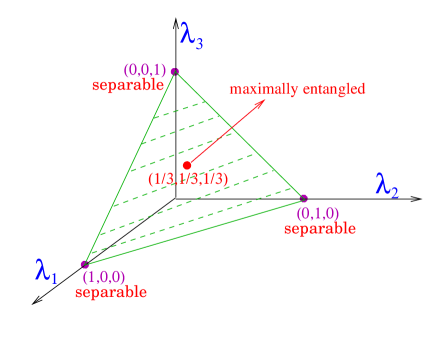
Figure 1.1: A cartoon for $N=3$. The system lives on the triangular plane $\lambda_{1}+\lambda_{2}+\lambda_{3}=1$. The vertices of the triangle represent the separable configurations and the centroid $(\lambda_{1}=\lambda_{2}=\lambda_{3}=1/3)$ represents the maximally entangled configuration.

If the system is in a given configuration $\{\lambda_{i}\}$ on the allowed plane $\sum_{i=1}^{N}\lambda_{i}=1$ (and $\lambda_{i}\geq 0$), how much entangled it is? In other words, how do we measure the entanglement content of a given configuration of $\{\lambda_{i}\}$? This is usually done by defining the so called entanglement entropy, a single scalar quantity associated with each configuration, i.e., each point on the plane $\sum_{i=1}^{N}\lambda_{i}=1$ (and $\lambda_{i}\geq 0$). A standard and perhaps most studied measure of entanglement is the so called von Neumann entropy [Ben96], $S_{1}=-\sum_{i=1}^{N}\lambda_{i}\ln(\lambda_{i})=-{\rm Tr}[\rho_{A}\ln(\rho_{A})]$, which has its smallest value $S_{1}=0$ in configuration (i) and its maximum possible value $S_{1}=\ln N$ in configuration (ii). Renyi entropy defined as $S_{q}=\ln\left(\sum_{i}\lambda_{i}^{q}\right)/(1-q)$ [Ren70] with the parameter $q>0$ is a natural generalization that reduces to the von Neumann entropy when $q\to 1$. Again, for any $q>0$, $S_{q}=0$ at the ‘separable’ vertices (situation (i) above) and $S_{q}=\ln(N)$ at the ‘maximally entangled’ centroid (situation (ii) above). For $q=2$, $\sum_{i=1}^{N}\lambda_{i}^{2}=\exp[-S_{2}]$ is called the purity that has been widely studied (see [Fac06] and references therein). For other measures we refer the reader to the introduction in [Gir07]. Essentially, one can define any scalar quantity whose value increases monotonically as one moves from fully ‘separable’ to maximally ‘entangled’ configurations (e.g., as one moves from the vertices towards the centroid in Fig. (1.1)) (for more detailed prescriptions and requirements on the measure, see e.g.  [Ved98]).

Important informations regarding the degree of entanglement can also be obtained from the two extreme eigenvalues, the largest $\lambda_{\rm max}={\rm max}(\lambda_{1},\lambda_{2},\ldots,\lambda_{N})$ and the smallest $\lambda_{\rm min}={\rm min}(\lambda_{1},\lambda_{2},\ldots,\lambda_{N})$. Due to the constraint $\sum_{i=1}^{N}\lambda_{i}=1$ and the fact that eigenvalues are all non-negative, it follows that $1/N\leq\lambda_{\rm max}\leq 1$ and $0\leq\lambda_{\rm min}\leq 1/N$. Consider, for instance, the following limiting situations. Suppose that the largest eigenvalue $\lambda_{\rm max}={\rm max}(\lambda_{1},\lambda_{2},\ldots,\lambda_{N})$ takes its maximum allowed value $1$. Then due to the constraint $\sum_{i=1}^{N}\lambda_{i}=1$ and the fact that $\lambda_{i}\geq 0$ for all $i$, it follows that all the rest $(N-1)$ eigenvalues must be identically $0$. Thus it corresponds to the configuration (i) above of fully separable state. On the other hand, if $\lambda_{\rm max}=1/N$ (i.e., it takes its lowest allowed value), it follows that all the eigenvalues must have the same value, $\lambda_{i}=1/N$ for all $i$, again due to the constraint $\sum_{i=1}^{N}\lambda_{i}=1$. This then corresponds to situation (ii) of maximally entangled state. Thus, for instance, one can consider $-\ln(\lambda_{\rm max})$ as a measure of entanglement as it increases from its value $0$ in the separable state to its maximal value $\ln(N)$ in the maximally entangled case. In fact, $-\ln(\lambda_{\rm max})$ is precisely the $q\to\infty$ limit of the Renyi entropy $S_{q}$.

In this chapter our particular interest is on the smallest eigenvalue $0\leq\lambda_{\rm min}\leq 1/N$. When $\lambda_{\rm min}$ takes its maximal allowed value $1/N$, it follows again, from the constraint $\sum_{i=1}^{N}\lambda_{i}=1$ and $\lambda_{i}\geq 0$ for all $i$, that all the eigenvalues must have the same value $\lambda_{i}=1/N$. This will thus make the state $|\psi\rangle$ maximally entangled, i.e., situation (ii). In the opposite case, when $\lambda_{\rm min}$ takes its smallest allowed value $0$, while it does not provide any information on the entanglement of the state $|\psi\rangle$, one sees from the Schmidt decomposition (1.3.9) that the dimension of the effective Hilbert space of the subsystem $A$ reduces from $N$ to $N-1$ (assuming that $\lambda_{\rm min}$ is non-degenerate). Indeed, if $\lambda_{\rm min}$ is very close to zero, one can effectively ignore the term containing $\lambda_{\rm min}$ in Eq. (1.3.9) and achieve a reduced Hilbert space, a process called ‘dimensional reduction’ that is often used in the compression of large data structures in computer vision [Wil62, Fuk90, Viv07]. Thus the knowledge of $\lambda_{\rm min}$ and in particular its proximity to its upper and lower limits provide informations on both the degree of entanglement as well as on the efficiency of the dimensional reduction process.

Random Pure State: So far, our discussion was valid for an arbitrary pure state in Eq. (1.3.1) with any fixed coefficient matrix $X=[x_{i,\alpha}]$. One can now introduce a statistical measure or distribution for the entries of the matrix $X$ which, in turn, will induce a probability distribution for the eigenvalues $\lambda_{i}$’s of $W=XX^{\dagger}$ that appear in the Schimdt representation in Eq. (1.3.9). As a result, any measure of entanglement (e.g., the von Neumann entropy or the minimum eigenvalue $\lambda_{\rm min}$) will also have a statistical distribution associated with it. The main challenge then is to compute this probability distribution of the entanglement, given the measure on the entries of $X$.

So, what is an appropriate measure on $X$? Evidently, we can not choose any arbitrary measure on $X$. Indeed, in Eq. (1.3.1) we can just rotate (unitarily) the basis of the Hilbert space. Clearly physical properties of the system in a pure state should not depend on which basis we choose. Thus the joint probability distribution of the entries $x_{i,\alpha}$ in Eq. (1.3.1) should be invariant under a unitary (or orthogonal if we restrict $X$ to be real) transformation $|\psi\rangle\to U|\psi\rangle$, where $U$ represents a unitary operator. The only measure that remains invariant under a unitary rotation is the uniform measure over all pure states. This is the so called Haar measure where the coefficients $x_{i,\alpha}$’s are uniformly distributed over all possible values satisfying the constraint $\sum_{i,\alpha}|x_{i,\alpha}|^{2}=1$ or equivalently, $P[\{X_{ij}\}]\propto\delta\left({\rm Tr}(XX^{\dagger}-1\right)$. The physical meaning of this Haar measure is clear: under unitary time evolution, and in absence of any other conservation law (such as fixed energy as in the case of standard microcanonical ensemble in statistical physics), the system visits all allowed normalized pure states equally likely, i.e., Haar measure is a natural stationary measure under unitary evolution when ergodicity holds over all allowed pure states of the composite system. This is, in fact, the case in many physical situations when the system is described by a sufficiently complex ‘time-dependent’ Hamiltonian as in quantum chaotic systems [Ban02].

Given that the entries of $X$ are distributed via the Haar measure $P[\{X_{ij}\}]\propto\delta\left({\rm Tr}(XX^{\dagger}-1\right)$, the next question is how are the eigenvalues of $W=XX^{\dagger}$ distributed? Noticing that the eigenvalues $\lambda_{i}$’s of $W=XX^{\dagger}$ are the same as Wishart eigenvalues, except with the additional constraint ${\rm Tr}(W)=\sum_{i=1}^{N}\lambda_{i}=1$, it follows immediately from Eq. (1.2.1) that the joint pdf of $\lambda_{i}$’s is given by [Llo88, Zyc01]

$$P[\{\lambda_{i}\}]=B_{M,N}\delta\left(\sum_{i=1}^{N}\lambda_{i}-1\right)\prod_{i=1}^{N}\lambda_{i}^{\frac{\beta}{2}(M-N+1)-1}\prod_{j<k}|\lambda_{j}-\lambda_{k}|^{\beta}$$ (1.3.10)

where the normalization constant $B_{M,N}$ is known explicitly [Zyc01]. Note that the exponential factor $e^{-\frac{\beta}{2}\sum_{i=1}^{N}\lambda_{i}}$ present in Eq. (1.2.1) becomes a constant due to the constraint $\sum_{i=1}^{N}\lambda_{i}=1$ and hence is absorbed in the normalization constant $B_{M,N}$. The ensemble described in Eq. (1.3.10) can thus be seen as the microcanonical version of the canonical Wishart ensemble in (1.2.1).

When the coefficient matrix $X$ is drawn from the Haar measure, we will refer to the state in Eq. (1.3.1) as a random pure state. Given that $\lambda_{i}$’s corresponding to the random pure state are distributed via the joint pdf (1.3.10), it follows that the associated observables such as the von Neumann entropy $S_{1}=-\lambda_{i}\ln(\lambda_{i})$, the maximum eigenvalue $\lambda_{\rm max}$, the minimum eigenvalue $\lambda_{\rm min}$ etc. are also random variables. The main technical problem then is to evaluate the statistical properties (such as the mean, variance or even the full probability distribution) of such observables.

There have been quite a few studies in this direction. For example, the average entropy $\langle S_{1}\rangle$ (where the average is performed with the measure in Eq. (1.3.10)) was computed for $\beta=2$ by Page [Pag95] and was found to be $\langle S\rangle\approx\ln(N)-\frac{N}{2M}$ for large $1<<N\leq M$. Noting that $\ln(N)$ is the maximal possible value of entropy of the subsystem $A$, the average entanglement entropy of a random pure state was concluded to be near maximal. Later, the same result was shown to hold for the $\beta=1$ case [Ban02]. On the other hand, there have been only few studies on the full probability distribution of the entanglement entropy. The distribution of the so called G-concurrence [Cap06], a measure of entanglement, was computed exactly in the large $N$ limit and was shown to have a point measure (delta function). For small $N$, the distribution of purity is known [Gir07]. On the other hand, for large $N$, the Laplace transform of the distribution of purity (for positive Laplace variable) was computed in  [Fac08, Pas09] which only gave partial information about the full purity distribution.

Recently, using a Coulomb gas approach, the full probability distribution of the Renyi and von Neumann entropy, as well as that of purity, was computed exactly in the large $N$ limit by studying the associated Coulomb gas model via a saddle point method [Nad10]. Interestingly, the pdf of the entropy exhibits two singular points which correspond to two interesting phase transitions in the Coulomb gas problem [Nad10, Fac08, Pas09]. Similar phase transitions in the Coulomb gas picture, leading to a nonsingular pdf of a physical observable, have also been noted recently in several other problems where the random matrix theory is applicable: these include the pdf of the conductance and the shot noise power through a mesoscopic cavity [Viv08, Viv10, Osi08] (see also the chapter 35 and 36 of this book for applications of the RMT to quantum transport properties), the pdf of the number of positive eigenvalues (the so called index) of Gaussian random matrices [Maj09b], nonintersecting Brownian interfaces near a hard wall [Nad09] and in information and communication systems [Kaz09] to name a few.

Here our focus is on the statistical properties of the minimum eigenvalue $\lambda_{\rm min}$ and for all values of $M=N$. For the special case $\beta=2$ and $M=N$, the average value $\langle\lambda_{\rm min}\rangle$ was studied recently by Znidaric [Zni07]. He computed, by hand, $\langle\lambda_{\rm min}\rangle$ for small values of $N$ and conjectured that $\langle\lambda_{\rm min}\rangle=1/N^{3}$ for all $N$. Later, in [Maj08], the full probability distribution of $\lambda_{\rm min}$ was computed explicity for all $M=N$ and $\beta=1$ and $\beta=2$. Znidaric’s conjecture for $\beta=2$ then followed as a simple corollary [Maj08]. In the next section, I briefly outline this derivation and also provide a new result for the distribution of $\lambda_{\rm min}$ for $\beta=4$.

1.4 Minimum Eigenvalue Distribution for $M=N$

In this section, we compute the distribution of $\lambda_{\rm min}$ when the eigenvalues are distributed via Eq. (1.3.10). It is easier to compute the cumulative distribution

$$R_{N}(x)=\mbox{Prob}\left[\lambda_{\rm min}\geq x\right]=\mbox{Prob}\left[\lambda_{1}\geq x,\lambda_{2}\geq x,\ldots,\lambda_{N}\geq x\right].$$ (1.4.1)

Using (1.3.10)

$$R_{N}(x)=B_{M,N}\,\int_{x}^{\infty}\cdots\int_{x}^{\infty}\delta\left(\sum_{i=1}^{N}\lambda_{i}-1\right)\prod_{j<k}|\lambda_{j}-\lambda_{k}|^{\beta}\,\prod_{i=1}^{N}\lambda_{i}^{\frac{\beta}{2}(M-N+1)-1}\,d\lambda_{i}.$$ (1.4.2)

The challenge is to evaluate this multiple integral.

We proceed by introducing an auxiliary integral

$$I(x,t)=\int_{x}^{\infty}\cdots\int_{x}^{\infty}\delta\left(\sum_{i=1}^{N}\lambda_{i}-t\right)\prod_{j<k}|\lambda_{j}-\lambda_{k}|^{\beta}\,\prod_{i=1}^{N}\lambda_{i}^{\frac{\beta}{2}(M-N+1)-1}\,d\lambda_{i}.$$ (1.4.3)

If we can evaluate $I(x,t)$ for all $t$, then

$$R_{N}(x)=B_{M,N}\,I(x,1).$$ (1.4.4)

To evaluate $I(x,t)$, it is natural to consider its Laplace transform

$$\int_{0}^{\infty}I(x,t)e^{-st}dt=\int_{x}^{\infty}\cdots\int_{x}^{\infty}e^{-s\sum_{i=1}^{N}\lambda_{i}}\prod_{j<k}|\lambda_{j}-\lambda_{k}|^{\beta}\,\prod_{i=1}^{N}\lambda_{i}^{\frac{\beta}{2}(M-N+1)-1}\,d\lambda_{i}.$$ (1.4.5)

Next, a change of variable $\lambda_{i}=\frac{\beta}{2s}\,w_{i}$ reduces it to

$$\int_{0}^{\infty}I(x,t)e^{-st}dt=\left(\frac{\beta}{2s}\right)^{-\beta MN/2}\,\int_{2sx/\beta}^{\infty}\dots\int_{2sx/\beta}^{\infty}e^{-\frac{\beta}{2}\sum_{i=1}^{N}w_{i}}\,\prod_{j<k}|w_{j}-w_{k}|^{\beta}\,\prod_{i=1}^{N}w_{i}^{\alpha\beta/2}\,dw_{i}$$ (1.4.6)

where $\alpha=(1+M-N)-2/\beta$. Next we recognize the multiple integral, up to an overall constant, as the cumulative distribution $Q_{N}(2sx/\beta)$ of the minimum eigenvalue $w_{\rm min}$ in the unconstrained Wishart ensemble discussed previously. Thus, up to an overall constant $A_{1}$ independent of $s$, we have

$$\int_{0}^{\infty}I(x,t)e^{-st}dt=A_{1}s^{-\beta MN/2}\,Q_{N}\left(\frac{2sx}{\beta}\right).$$ (1.4.7)

The program then is to invert this Laplace transform, compute $I(x,t)$ for all $t$ and calculate $R_{N}(x)$ using Eq. (1.4.4). Henceforth, we will drop the overall constant which can be finally fixed from the normalization that $R_{N}(0)=1$.

Thus, if we know the cumulative distribution of the Wishart minimum eigenvalue $Q_{N}(z)$, we can, at least in principle, determine the minimum eigenvalue distribution $R_{N}(x)$ for the random pure state problem. This is hardly surprising given the microcanonical to canonical correspondence between the two ensembles. In practice, however, it is nontrivial to invert the Laplace transform in Eq. (1.4.7). That indeed is the real challenge. We will see below that fortunately for $M=N$, where $Q_{N}(z)$ is given in Eqs. (1.2.9), (1.2.8) and (1.2.10) for $\beta=1$, $2$ and $4$ respectively, this Laplace inversion can be carried out in closed form and one can compute $R_{N}(x)$ explicitly in all three cases $\beta=1$, $2$ and $4$.

The case $\beta=2$: Let us start with the simplest case $\beta=2$ with $M=N$. Here $Q_{N}(z)=e^{-Nz}$ from Eq. (1.2.8). Dropping the overall constant, Eq. (1.4.7) gives

$$\int_{0}^{\infty}I(x,t)e^{-st}dt=\dfrac{e^{-sNx}}{s^{N^{2}}}.$$ (1.4.8)

The Laplace inversion is trivial upon using the convolution theorem giving (up to an overall constant) $I(x,t)=(t-Nx)^{N^{2}-1}\Theta(t-Nx)$ where $\Theta(z)$ is the step function. Putting $t=1$ and using (1.4.4) gives the exact distribution [Maj08]

$$R_{N}(x)=\mbox{Prob}\left[\lambda_{\rm min}\geq x\right]=\left(1-Nx\right)^{N^{2}-1}\Theta\left(1-Nx\right).$$ (1.4.9)

Subsequently, the pdf is given by

$$P_{N}(x)=-\frac{dR_{N}(x)}{dx}=N(N^{2}-1)(1-Nx)^{N^{2}-2}\,\Theta(1-Nx).$$ (1.4.10)

A plot of this pdf can be found in Fig. (1.2) for $N=2$. Thus $P_{N}(x)$ in $x\in[0,1/N]$ has the limiting behavior

$$P_{N}(x) \to N\,(N^{2}-1)\quad\quad{\rm as}\quad x\to 0$$ (1.4.11)

$$\to N\,(N^{2}-1)\,(1-Nx)^{N^{2}-2}\quad{\rm as}\quad x\to 1/N$$

One can easily compute all the moments explicitly

$$\mu_{k}(N)=\langle\lambda_{\rm min}^{k}\rangle=\int_{0}^{\infty}x^{k}P_{N}(x)\,dx=\frac{\Gamma(k+1)\Gamma(N^{2})}{N^{k}\,\Gamma(N^{2}+k)}.$$ (1.4.12)

In particular, for $k=1$, we obtain for all $N$

$$\mu_{1}(N)=\langle\lambda_{\rm min}\rangle=\frac{1}{N^{3}},$$ (1.4.13)

proving the conjecture by Znidaric [Zni07]. Putting $k=2$ in Eq. (1.4.12), we get the second moment $\mu_{2}=\frac{2}{N^{4}(N^{2}+1)}$. Thus the variance is given by

$$\sigma^{2}=\mu_{2}(N)-[\mu_{1}(N)]^{2}=\frac{1}{N^{6}}\left(\frac{N^{2}-1}{N^{2}+1}\right).$$ (1.4.14)

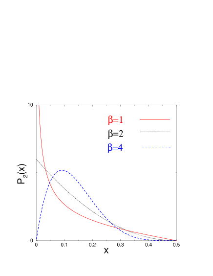
Figure 1.2: The pdf of $\lambda_{\rm min}$ for $N=2$ for $\beta=1$, $\beta=2$ and $\beta=4$.

The case $\beta=1$: The computation in this case proceeds as in the case $\beta=2$, though the Laplace inversion is nontrivial. Omitting details [Maj08], we just quote here the main results. For $M=N$, the pdf of the minimum eigenvalue, $P_{N}(x)=-dR_{N}(x)/dx$ is nonzero in $x\in[0,1/N]$ and is given by [Maj08]

$$P_{N}(x)=A_{N}\,x^{-N/2}\,(1-Nx)^{(N^{2}+N-4)/2}\,_{2}F_{1}\left(\frac{N+2}{2},\frac{N-1}{2},\frac{N^{2}+N-2}{2},-\frac{1-Nx}{x}\right)$$ (1.4.15)

where ${}_{2}F_{1}(a,bc,c,z)$ is the standard hypergeometric function [Abr72] and the constant $A_{N}$ is given by

$$A_{N}=\dfrac{N\,\Gamma(N)\,\Gamma(N^{2}/2)}{2^{N-1}\,\Gamma(N/2)\,\Gamma((N^{2}+N-2)/2)}.$$ (1.4.16)

The limiting behavior of $P_{N}(x)$ as $x\to 0$ and $x\to 1/N$ can be worked out

$$P_{N}(x) \approx \left[\frac{\sqrt{\pi}\,\Gamma(N)\,\Gamma(N^{2}/2)}{2^{N-1}\,\Gamma^{2}(N/2)\,\Gamma((N-1)/2)}\right]\,x^{-1/2}\quad\,{\rm as}\quad x\to 0$$ (1.4.17)

$$\approx A_{N}\,N^{-N/2}\,(1-Nx)^{(N^{2}+N-4)/2}\quad\,{\rm as}\quad x\to 1/N$$

All moments can also be worked out explicitly [Maj08]. In particular, the average is given by

$$\mu_{1}(N)=\langle\lambda_{\rm min}\rangle=\frac{\sqrt{\pi}\,\Gamma(N)}{N\,\Gamma(N/2)\,\Gamma((N+5)/2)2^{N-1}}\,_{2}F_{1}\left(3,\frac{3}{2},\frac{N+5}{2},1-N\right).$$ (1.4.18)

Thus the expression for $\langle\lambda_{\rm min}\rangle$ for arbitrary $N$ in the real $(\beta=1)$ case is considerably more complicated than its counterpart in Eq. (1.4.13) for the complex case. One finds, from Eq. (1.4.18), that $\mu_{1}(N)$ decreases with increasing $N$, e.g., $\mu_{1}(1)=1$, $\mu_{1}(2)=(4-\pi)/8$, $\mu_{1}(3)=(2-\sqrt{3})/9$ etc. One can show [Maj08] that asymptotically for large $N$, $\mu_{1}(N)$ decays as

$$\mu_{1}(N)\approx\frac{c_{1}}{N^{3}}$$ (1.4.19)

where $c_{1}$ is precisely the constant in Eq. (1.2.16).

The case $\beta=4$: For $\beta=4$, we first substitute $Q_{N}(z)$ from (1.2.10) in (1.4.7), expand the hypergeometric function in power series as in (1.2.11) and then invert the Laplace transform term by term to get a series for $I(x,t)$. To transform each term, we make use of the convolution theorem. We then put $t=1$ in the expression for $I(x,t)$ and compute $R_{N}(x)$ in (1.4.4). The overall constant is fixed by imposing $R_{N}(0)=1$. This gives the explicit expression, valid for $0\leq x\leq 1/N$,

$$R_{N}(x)=\Gamma(N+1)\Gamma(2N^{2})\,\sum_{k=0}^{N}\frac{(2x)^{k}\,(1-Nx)^{2N^{2}-k-1}}{(N-k)!(2k)!\Gamma(2N^{2}-k)}$$ (1.4.20)

The pdf $P_{N}(x)=-dR_{N}(x)/dx$ of $\lambda_{\rm min}$ vanishes linearly at $x=0$ as $P_{N}(x)\to B_{N}\,x$ where $B_{N}=N(2N+1)(2N^{2}-1)(2N^{2}-2)/3$. This in contrast to the $\beta=1$ case (where $P_{N}(x)$ diverges as $x^{-1/2}$ as $x\to 0$) and also to the $\beta=2$ case where $P_{N}(x)$ approaches a constant as $x\to 0$ (see Fig. (1.2)). At the upper edge, when $x\to 1/N$, the pdf vanishes as $P_{N}(x)\sim(1-Nx)^{2N^{2}-N-2}$.

All the moments can also be calculated explicitly for $\beta=4$. For example, the average is given by

$$\mu_{1}(N)=\langle\lambda_{\rm min}\rangle=\frac{1}{2N^{3}}\sum_{k=0}^{N}{N\choose k}\,\frac{(k!)^{2}}{(2k)!}\,\left(\frac{2}{N}\right)^{k}.$$ (1.4.21)

One can extract the large $N$ asymptotics of this sum. We first express ${N\choose k}=\Gamma(N+1)/\Gamma(N-k+1)$, then use the property of the Gamma function, $\lim_{z\to\infty}\Gamma(z+a)/\Gamma(z)\to z^{a}$, to obtain for large $N$

$$\mu_{1}(N)=\langle\lambda_{\rm min}\rangle=\frac{1}{2N^{3}}\sum_{k=0}^{\infty}\frac{k!}{(2k)!}\,2^{k}$$ (1.4.22)

The sum can be exactly evaluated giving,

$$\mu_{1}(N)=\langle\lambda_{\rm min}\rangle\approx\frac{c_{4}}{N^{3}}$$ (1.4.23)

where $c_{4}$ is precisely the constant in Eq. (1.2.18).

Let us then summarize the behavior of the pdf $P_{N}(\lambda_{\rm min})$ of $\lambda_{\min}$ in the three cases $\beta=1$, $\beta=2$ and $\beta=4$ (see Fig. (1.2)). At the lower edge $x\to 0$, $P_{N}(x)$ displays very different behavior in the three cases. As $x\to 0$, $P_{N}(x)$ diverges as $x^{-1/2}$ for $\beta=1$, approaches a constant for $\beta=2$ and vanishes linearly for $\beta=4$. On the other hand, at the upper edge $x\to 1/N$, $P_{N}(x)$ approaches $0$ as a power law in all three cases, albeit with different powers, $P_{N}(x)\sim(1-Nx)^{\nu_{\beta}}$ where $\nu_{1}=(N^{2}+N-4)/2$, $\nu_{2}=N^{2}-2$ and $\nu_{4}=2N^{2}-N-2$.

In the large $N$ limit and in the range $x<<1/N$ (far away from the upper edge) the cumulative distribution $R_{N}(x)=\int_{x}^{1/N}P_{N}(x^{\prime})\,dx^{\prime}$ approaches the scaling form $R_{N}(x)\to q_{\beta}(xN^{3})$, where the scaling functions $q_{\beta}(y)$ are exactly same as in the unconstrained Wishart case given respectively in Eqs. (1.2.12), (1.2.13) and (1.2.14). Thus, in this range and for large $N$, effectively the random variable $\lambda_{\rm min}$ in the bipartite problem behaves, in law, as the Wishart minimum eigenvalue scaled by a factor $N^{-2}$, i.e., $\lambda_{\min}\to w_{\rm min}/N^{2}$. This is also confirmed in Eq. (1.2.5), where we see that the average trace in the unconstrained Wishart ensemble scales as $N^{2}$. Thus, in the microcanonical enemble, where the trace is constrained to be unity, it amounts to rescale all the Wishart eigenvalues by a factor $N^{-2}$ for large $N$. However, for finite $N$, the distributions are very different in the constrained and unconstrained ensembles, in particular near the upper edge $x=1/N$. In other words, the distribution of $\lambda_{\rm min}$ exhibits strong finite size effects.

1.5 Summary and Conclusion

In this chapter we have discussed an application of Wishart matrices in an entangled random pure state of a bipartite system consisting of two subsystems whose Hilbert spaces have dimensions $M$ and $N$ respectively with $N\leq M$. The $N$ eigenvalues of the reduced density matrix of the smaller subsystem are distributed exactly as the eigenvalues of a Wishart matrix, with the only difference that the eigenvalues satisfy a global constraint: the trace is fixed to be unity.

We have studied the distribution of the minimum eigenvalue in this fixed-trace Wishart ensemble. For the hard edge case (when two subsystems have same size $M=N$), we have shown that the minimum eigenvalue distribution can be computed exactly for all $N$ in all three interesting physical cases $\beta=1$, $\beta=2$ and $\beta=4$.

What does this exact distribution of $\lambda_{\rm min}$ tell us about the entanglement entropy of the bipartite system in a pure state? We have seen before that if $\lambda_{\rm min}$ is close to its maximally allowed value $1/N$ (set by the unit trace constraint), then that configuration is maximally entangled since all the eigenvalues contribute equally to the composition of the state. A measure of how close the random state is to this maximally entangled state can be estimated by computing the net measure of $\lambda_{\rm min}$ in a small range close to $1/N$, e.g., by the cumulative probability $R_{N}(1/N-\epsilon)=\int_{1/N-\epsilon}^{1/N}P_{N}(x)\,dx$ where $\epsilon<<1/N$. From our exact calculation, we see that the pdf of $\lambda_{\rm min}$, in all three cases, approaches zero as $\lambda_{\rm min}$ approaches its maximum possible value $1/N$, $P_{N}(\lambda_{\rm min}=x,N)\sim(1-Nx)^{\nu_{\beta}}$ where $\nu_{1}=(N^{2}+N-4)/2$, $\nu_{2}=N^{2}-2$ and $\nu_{4}=2N^{2}-N-2$. This shows that the ‘closeness to maximal entropy’ measure $R_{N}(1/N-\epsilon)\sim(\epsilon\,N)^{\nu_{\beta}+1}$. For $\epsilon<<1/N$, this measure is evidently very small. It was argued before [Pag95], on the basis of the computation of the only the first moment of the von Neumann entropy (not the full distribution), that a random state is almost maximally entangled. Our result shows that the probability that a random state is maximally entangled is actually very small. The same conclusion was also deduced recently on the basis of the large $N$ computation of the full distribution of the Renyi entropy [Nad10]. Thus, the lesson is that conclusions based just on the first moment, may sometimes be a bit misleading.

Here we have discussed only the hard edge $M=N$ case where the two subsystems have equal sizes. Our results are of relevance for small systems such as when each subsystem consists of identical number of qubits. It would be interesting to extend these calculations to the cases when $M\neq N$. In particular, in the context of thermodynamic systems where, for instance, one of the subsystems is a heat bath, one needs to study the opposite limit $N<<M$. It would be interesting to estimate the distribution of the minimum eigenvalue and other measures of entanglement in that limit.

Finally, we have restricted ourselves here to ‘random pure’ states where all pure states are sampled equally likely. This is the Haar measure. So far, we have not discussed dynamics, i.e., the temporal unitary evolution of the system. Under any unitary evolution that is ergodic over the space of all pure states, Haar measure is the unique stationary measure of the unitary evolution. This ergodicity holds provided one does not have any strict conservation law. For instance, the uniform measure over all pure states will not hold under the standard microcanonical scenario where the composite system has a fixed total energy $E$ (eigenvalue of the Hamiltonian $\hat{H}$ of the composite system). Only those pure states with total energy $E$, and not all pure states, will be sampled by the system under unitary evolution. An appropriate ‘stationary’ measure is then the microcanonical measure which is uniform over all pure states belonging to the fixed $E$ manifold. For such a measure, one can again define the reduced density matrix of the subsystem $A$ and its eigenvalues. It would be interesting to study the statistics of the bipartite entanglement (von Neumann or the Renyi entropy or the minimum eigenvalue $\lambda_{\rm min}$) in this microcanonical setting with a fixed total energy $E$. For such systems, some recent results of very general nature (that do not require the detailed knowledge of the Hamiltonian of the system) have been derived [Pop06, Gol06, Rei07] which says that any pure state, drawn from the uniform measure on the constrained manifold, will almost surely be ‘maximally entangled’ i.e., very close to the maximally entangled (centroid) configuration $\lambda_{i}=1/N$ for all $i$, provided $M>>N$, i.e., the environment (subsystem $B$) is much bigger than the system (subsystem $A$). It would be interesting to compute explicitly the distribution of this ‘typicality’ i.e, the distance between the pure state (drawn from a uniform measure over the constrained manifold) and the maximally entangled state for some systems with specific Hamiltonians.

Acknowledgements: The discussion in this chapter is based on my joint work [Maj08, Nad10, Viv07] with O. Bohigas, A. Lakshminarayan, C. Nadal, M. Vergassola and P. Vivo. It is my pleasure to thank them. I am particularly grateful to C. Nadal for carefully reading and correcting the manuscript. I also thank my other collaborators on related subjects in random matrix theory: A. Comtet, D.S. Dean, A. Scardicchio, and G. Schehr. After this article was accepted, I came across a recent preprint by Y. Chen, D.-Z. Liu and D.-S. Zhou (arXiv: 1002.3975) where the distribution of $\lambda_{\rm min}$ was computed for $M>N$ and for all $\beta$. Also, the average density of eigenvalues for all finite $N$ and $M$ but for $\beta=1$ was computed in a recent preprint of P. Vivo.

References

- [Abr72] M. Abramowitz and I.A. Stegun, Handbook of Mathematical Functions (Dover, New York, 1972)
- [Ake97] G. Akemann, Nucl. Phys. B507 (1997) 475
- [Ake08] G. Akemann and P. Vivo, JSTAT P09002 (2008)
- [Alt00] O. Alter et. al. Proc. Nat. Acad. Sci. USA 97 (2000) 10101
- [Amb94] J. Ambjorn, Yu. Makeenko, and C.F. Kristjansen, Phys. Rev. D50 (1994) 5193
- [Ban02] J. N. Bandyopadhyay and A. Lakshminarayan, Phys. Rev. Lett. 89 (2002) 060402
- [Ben01] G. Ben-Arous, A. Dembo, and A. Guionnet, Probab. Theory Relat. Fields 120 (2001) 1
- [Ben96] C.H. Bennet et. al. Phys. Rev. A bf 53 (1996) 2046
- [Boh84] O. Bohigas, M.-J. Giannoni, and C. Schmit, Phys. Rev. Lett. 52 (1984) 1
- [Bou01] J.-P. Bouchaud and M. Potters, Theory of Financial Risks (Cambridge University Press, Cambridge, 2001)
- [Bro65] B.V. Bronk, J. Math. Phys. 6 (1965) 228
- [Bur04] Z. Burda and J. Jurkiewicz, Physica A344 (2004) 67
- [Cap06] V. Cappellini, H.-J Sommers, and K. Zyczkowski, Phys. Rev. A 74 (2006) 062322
- [Che96] Y. Chen and S.M. Manning, J. Phys. A.: Math. Gen. 29 (1996) 7561
- [Dea06] D.S. Dean and S.N. Majumdar, Phys. Rev. Lett. 97 (2006) 160201; Phys. Rev. E 77 (2008) 041108
- [Ede88] A. Edelman, J. Matrix Anal. and Appl. 9 (1988) 543; Linear Algebra Appl. 159 (1991) 55
- [Fac06] P. Facchi, G. Florio, and S. Pascazio, Phys. Rev. A 74 (2006) 042331
- [Fac08] P. Facchi et. al. Phys. Rev. Lett. 101 (2008) 050502
- [For93] P.J. Forrrester, Nucl. Phys. B402 (1993) 709
- [For94] P.J. Forrester, J. Math. Phys. 35 (1994) 2539
- [Fuk90] K. Fukunaga, Introduuction to Statistical Pattern Recognition (Elsevier, New York, 1990)
- [Fyo97] Y.V. Fyodorov and H.-J. Sommers, J. Math. Phys. 38 (1997) 1918
- [Gir07] O. Giraud, J. Phys. A.: Math. Theor. 40 (2007) 1053
- [Gol06] S. Goldstein, J.L. Lebowitz, R. Tumulka, and N. Zanghi, Phys. Rev. Lett. 96 (2006) 050403
- [Hay06] P. Hayden, D. W. Leung and A. Winter, Comm. Math. Phys. 265 (2006) 95
- [Hol00] N. Holter et. al. Proc. Nat. Acad. Sci. USA 97 (2000) 8409
- [Jam64] A.T. James, Ann. Math. Stat. 35 (1964) 475
- [Joh00] K. Johansson, Comm. Math. Phys. 209 (2000) 437
- [Joh01] I.M. Johnstone, Ann. Statist. 29 (2001) 295
- [Kat03] M. Katori, H. Tanemura, T. Nagao, and N. Komatsuda, Phys. Rev. E68 (2003) 021112
- [Kaz09] P. Kazakopoulos et. al. arXiv:0907.5024
- [Llo88] S. Lloyd and H. Pagels, Ann. Phys. (NY) 188 (1988) 186
- [Maj08] S.N. Majumdar, O. Bohigas, and A. Lakshminarayan, J. Stat. Phys. 131 (2008) 33
- [Maj09a] S.N. Majumdar and M. Vergassola, Phys. Rev. Lett. 102 (2009) 060601
- [Maj09b] S.N. Majumdar, C. Nadal, A. Scardicchio, and P. Vivo, Phys. Rev. Lett. 103 (2009) 220603
- [Mar67] V.A. Marcenko and L.A. Pastur, Math. USSR-Sb 1 (1967) 457
- [Meh04] M.L. Mehta, Random Matrices (Academic Press, 3rd Edition, London, 2004)
- [Nad09] C. Nadal and S.N. Majumdar, Phys. Rev. E79 (2009) 061117
- [Nad10] C. Nadal, S.N. Majumdar, and M. Vergassola, Phys. Rev. Lett. 104 (2010) 110501
- [Nag93] T. Nagao and K. Slevin, J. Math. Phys. 34 (1993) 2075
- [Nag95] T. Nagao and P.J. Forrester, Nucl. Phys. B435 (1995) 401
- [Nov08] J. Novembre and M. Stephens, Nature Genetics 40 (2008) 646
- [Osi08] V. Al Osipov and E. Kanzieper, Phys. Rev. Lett. 101, 176804 (2008); Note that the results for the tails of the conductance pdf stated in this paper were errorneous and the correct results can be found in [Viv08] and [Viv10].
- [Pag95] D. N. Page, Phys. Rev. Lett. 71 (1995) 1291
- [Pas09] A. De Pasquale, P. Facchi, G. Parisi, S. Pascazio, and A. Scardicchio, arXiv:0911.3888
- [Pat06] N. Patterson, A.L. Preis, and D. Reich, PLos Gentics 2 (2006) 2074
- [Per93] A. Peres, Quantum Theory: Concepts and Methods, (Kluwer Academic Publishers, Dordrecht, 1993)
- [Pop06] S. Popescu, A.J. Short and A. Winter, Nature Physics, 2 (2006) 754
- [Pre88] R.W. Preisendorfer, Principal Component Analysis in Meteorology and Oceanography (Elsevier, New York, 1988)
- [Rei07] P. Reimann, Phys. Rev. Lett. 99 (2007) 160404
- [Ren70] A. Renyi, Probability Theory (North Holland, Amsterdam, 1970)
- [Sch08] G. Schehr, S.N. Majumdar, A. Comtet, and J. Randon-Furling, Phys. Rev. Lett. 101 (2008) 150601
- [Tra94] C. Tracy and H. Widom, Commun. Math. Phys. 159 (1994) 151; 177 (1996) 727
- [Ver94a] J.J.M. Verbaarschot, Phys. Rev. Lett. 72 (1994) 2531 and references therein
- [Ver94b] J.J.M. Verbaarschot, Nucl. Phys. B426 (1994) 559
- [Ved98] V. Vedral and M.B. Plenio, Phys. Rev. A 57 (1998) 1619
- [Viv07] P. Vivo, S.N. Majumdar, and O. Bohigas, J. Phys. A 40 (2007) 4317
- [Viv08] P. Vivo, S.N. Majumdar, and O. Bohigas, Phys. Rev. Lett. 101 (2008) 216809
- [Viv10] P. Vivo, S.N. Majumdar, and O. Bohigas, Phys. Rev. B. 81 (2010) 104202
- [Wil62] S.S. Wilks, Mathematical Statistics (John Wiley & Sons, New York, 1962)
- [Wis28] J. Wishart, Biometrica 20 (1928) 32
- [Zyc01] K. Zyczkowski and H-J. Sommers, J. Phys. A: Math. Gen. 34 (2001) 7111
- [Zni07] M. Znidaric, J. Phys. A: Math. Theor. 40 (2007) F105