Experimental investigation of the non-Markovian dynamics of classical and quantum correlations

Abstract

We experimentally investigate the dynamics of classical and quantum correlations of a Bell diagonal state in a non-Markovian dephasing environment. The sudden transition from classical to quantum decoherence regime is observed during the dynamics of such kind of Bell diagonal state. Due to the refocusing effect of the overall relative phase, the quantum correlation revives from near zero and then decays again in the subsequent evolution. However, the non-Markovian effect is too weak to revive the classical correlation, which remains constant in the same evolution range. With the implementation of an optical $\sigma_{x}$ operation, the sudden transition from quantum to classical revival regime is obtained and correlation echoes are formed. Our method can be used to control the revival time of correlations, which would be important in quantum memory.

I Introduction

Quantum entanglement, as a kind of distinctive quantum correlation without the classical counterpart, is widely recognized as the crucial resource of quantum communication and computation Nielsen00 . However, there are also other nonclassical correlations that can even exist in separated quantum states Ollivier01 ; Henderson01 . The finding that nonclassical correlations other than quantum entanglement may provide the speedup in the deterministic quantum computation with one pure qubit (DQC1) protocol Datta08 ; Lanyon08 has greatly motivated the related study.

One of the essential issues is to distinguish different kinds of correlations in quantum systems. In the classical information theory, correlation is perfectly characterized by the Shannon entropy, which is represented by the classical mutual information Shannon48 . When it comes to quantum systems, the Shannon entropy is replaced by the von Neumann entropy and the total correlation in a bipartite system is characterized by the quantum mutual information Groisman05 . For bipartite systems, the quantumness of correlation can be quantified by the quantum discord which represents the difference between classical information theory and quantum information theory Ollivier01 . A related method concerning classical correlation is proposed and it is based on the maximal information one can extract with a one-sided local measurement Henderson01 . It has been demonstrated that almost all quantum states contains non-vanishing quantum discord that is composed by the quantum entanglement and non-entanglement quantum correlation Ferraro10 .

There are many investigations of quantum correlation measured by quantum discord in different kinds of physical systems, including the spin chains Sarandy09 ; Werlang10 ; Chen10 ; Werlang102 , Jaynes-Cummings systems Cole10 , spin-boson systems Ge01 , optical systems Xu10 , quantum dots Fanchini-Castelano10 and NMR systems Soares10 . Recently, this kind of measurement is also extended to continuous variable systems Giorda10 ; Adesso10 ; Vasile10 and even the quantum biology systems Bradler10 . Quantum discord has been found to be useful in quantum information processing and quantum information theory. The non-entanglement quantum discord may provide the quantum advantage in the DQC1 quantum computation protocol Datta08 ; Lanyon08 . The vanishing of quantum discord implies completely positive dynamics maps Shabani09 . Quantum discord also plays important roles in many basic physical problems, for example the Maxwell’s demon Zurek03 , quantum phase transition Sarandy09 ; Werlang10 ; Chen10 ; Werlang102 and the relative effect Datta09 ; WangDeng10 .

The quantification of quantum discord is based on the one-sided measurement on a bipartite system, which is usually asymmetric. We would get different results by choosing different subsystem to be measured. A symmetrical method with two-sided measurement over both partitions of a bipartite system is proposed to quantify the classical correlation which is represented by the maximal classical mutual information Terhal02 ; DiVincenzo04 . There are also other approaches proposed to distinguish classical and quantum correlations. Inspired by the work consumption when extracting information from a heat bath, a thermodynamics approach is used to defined quantum correlation in quantum systems Oppenheim02 ; Horodecki05 . In particularly, the difference between the extractable information with the closed local operation and classical communication and the total information is defined as the quantum information deficit, which is used to quantify quantum correlation Horodecki05 . Because classical states are measured without disturbance, classical and quantum correlations are also characterized by the measurement-induced disturbance Luo08 . Recently, by employing the relative entropy as a distance measure of correlations, the method proposed by Modi et al. Modi10 provides an unified view of quantum and classical correlations. Different from quantum discord based on bipartite mutual information, this method can be extended to quantified different kinds of correlations in multipartite systems of arbitrary dimensions. Generally, all these measurements of classical and quantum correlations mentioned above are not equal to each other due to the different definitions. However, they are consistent in the case of distinguishing classical and quantum correlations in Bell diagonal states Xu10 .

Another interesting subject is to investigate the dynamics of different kinds of correlations in noisy environments. For one side, the inevitable interaction between a quantum system and its environment would destroy correlations in the system and leads to the reduction of useful resource. The knowledge of the dynamic behavior of correlations will help us to design suitable protocols to protect correlations under processing. For the other side, stimulated by the discovery of distinctive dynamic behavior of entanglement sudden death Yu09 , that is, entanglement disappear completely in a finite evolution time, the investigation of the unusual dynamic behavior of classical and quantum correlations has caused great interests. Usually, the dissipative correlation evolution is essentially dependent on the types of noises that act on the system. Markovian noises would cause the irreversible decay of system information into the environment. It has been shown that quantum discord is more robust than entanglement under Markovian noises Werlang09 , in the sense that entanglement may suffer from sudden death, whereas quantum correlation decays exponentially. The sudden change in behavior in the decay rates of classical and quantum correlations has been predicted in different kinds of Markovian environments Maziero09 and has been experimentally verified in an optical system Xu10 . The decoherence-free evolution of quantum and classical correlations under certain Markovian noise and the sudden transition from classical to quantum decoherence regime are also observed Xu10 ; Mazzola10 . The Markovian dynamics of classical and quantum correlations is also experimentally investigated in a nuclear magnetic resonance quadrupolar system Soares10 . When it is extended to the non-Markovian environment with memory effect, the feedback information from the environment to the interested system may greatly affect the dynamic behavior of correlations. Quantum discord under non-Markovian noises is shown to be instantaneously vanished compared to the completely disappearance of entanglement in a finite time interval Wang10 ; Fanchini10 . The revival of quantum discord without the revival of entanglement is also demonstrated in non-Markovian noises Werlang10 .

In this paper, based on the equal footing method with the relative entropy as a distance measurement of correlations, we experimentally investigate the dynamics of classical and quantum correlations of a two-photon Bell diagonal state in a one-sided non-Markovian environment, which is simulated by a Fabry-Perot cavity followed by quartz plates. At the beginning of evolution, the sudden transition from classical to quantum decoherence regime is shown Xu10 ; Mazzola10 . Due to the refocusing effect of the relative phase in the non-Markovian environment, the quantum correlation revives from a near zero area and then decays again in the subsequent evolution. However, the non-Markovian effect is too weak to revive the classical correlation, which remains constant at the same evolution range. We then perform a $\sigma_{x}$ operation on the photon under decoherence and the sudden transition from quantum to classical revival regime is obtained, in which correlation echoes are formed.

The paper is organized as follows. The measure of correlations using relative entropy and the theoretical description of the experiment are given in section II. The experimental setup and results are presented in section III. We then give a discussion and conclusion in section IV.

II Relative entropy of correlations and Theoretical description of the experiment

II.1 Relative Entropy of Correlations

The magnitude of a specified property in a quantum system can be quantified by the distance from the interested state to the closest state without that desired property Modi10 . For example, quantum entanglement can be characterized by the relative entropy of entanglement ($REE$) Vedral97 , which is described as the minimal distance measured with relative entropy between the state $\rho$ and a separated state $\sigma$ and is expressed as $REE=\underset{\sigma\in D}{\min}S(\rho||\sigma)$. $S(\rho||\sigma)=-\mbox{tr}(\rho\log_{2}\sigma)-S(\rho)$ and $S(\rho)=-\mbox{tr}(\rho\log_{2}\rho)=-\sum_{j}p_{j}\log_{2}p_{j}$ is the von Neumann entropy ($p_{j}$ represent the eigenvalues of $\rho$). D is the set of separable states. As a result, if all the distances are measured with relative entropy, different kinds of correlations in a quantum system can be measured on an equal footing. The quantum correlation is then defined as the minimal distance between $\rho$ and a classical state $\chi$, which is expressed as $\mathcal{Q}=\underset{\chi\in C}{\min}S(\rho||\chi)$ Modi10 . $C$ represents the set of classical states. Whereas the classical correlation is defined as the minimal distance between $\chi$ and a product state $\pi$ and is expressed as $\mathcal{C}=\underset{\pi\in P}{\min}S(\chi||\pi)$ Modi10 , where $P$ is the set of product states.

It has been demonstrated that the calculations of quantum and classical correlations in a quantum system ($\rho$) can be further simplified as Modi10

$$\mathcal{Q} = S(\chi_{\rho})-S(\rho),$$ (1)

$$\mathcal{C} = S(\pi_{\chi_{\rho}})-S(\chi_{\rho}),$$ (2)

where $\chi_{\rho}$ represents the closest classical state of $\rho$ and $\pi_{\chi_{\rho}}$ is the corresponding reduced state of $\chi_{\rho}$ in the product form which is the closest product state of $\chi_{\rho}$.

The total mutual information of $\rho$ can be calculated as

$$\mathcal{I}=S(\pi_{\rho})-S(\rho),$$ (3)

which represents the minimal distance between $\rho$ and its reduced state in the product form $\pi_{\rho}$ Modi10 . For bipartite systems, $\mathcal{I}$ is equal to the quantum mutual information.

Generally, it is difficult to find the closest classical state $\chi_{\rho}$. However, for the Bell diagonal state $\rho=\sum_{i=1}^{4}\lambda_{i}|\Phi_{i}\rangle\langle\Phi_{i}|$ where $\lambda_{i}$ are the non-increasing eigenvalues and $|\Phi_{i}\rangle$ represent the four Bell states, the analytic expression of $\chi_{\rho}$ is found and $\chi_{\rho}=\frac{\lambda_{1}+\lambda_{2}}{2}(|\Phi_{1}\rangle\langle\Phi_{1}|+|\Phi_{2}\rangle\langle\Phi_{2}|)+\frac{\lambda_{3}+\lambda_{4}}{2}(|\Phi_{3}\rangle\langle\Phi_{3}|+|\Phi_{4}\rangle\langle\Phi_{4}|)$ Modi10 . As a result, for the Bell diagonal state with the eigenvalues $\{\lambda_{1},\lambda_{2},\lambda_{3},\lambda_{4}\}$, the eigenvalues of the closest classical state is $\{\frac{1}{2}(\lambda_{1}+\lambda_{2}),\frac{1}{2}(\lambda_{1}+\lambda_{2}),\frac{1}{2}(\lambda_{3}+\lambda_{4}),\frac{1}{2}(\lambda_{3}+\lambda_{4})\}$. We can therefore calculate the quantum correlation $\mathcal{Q}$ according to equation (1). The product states of $\rho$ and $\chi_{\rho}$ are both identical and equal to the normalized identity $\openone/4$. As a result, the classical correlation and total mutual information can be calculated according to equations (2) and (3) respectively and $\mathcal{I}=\mathcal{Q}+\mathcal{C}$. The analytic solution of the relative entropy of entanglement for Bell diagonal states is given by Vedral97

$$REE=1+\lambda_{1}\log_{2}\lambda_{1}+(1-\lambda_{1})\log_{2}(1-\lambda_{1}),$$ (4)

if $\lambda_{1}\geq 1/2$, whereas

$$REE=0,$$ (5)

if $\lambda_{1}\in[0,1/2]$.

As a result, with the knowledge of $\rho$, one can compute different kinds of correlations.

II.2 Theoretical description of the experiment

The pure dephasing environment is a kind of uniquely quantum noise, which causes randomness between the relative phases of information carries. In optical systems, the coupling between the photon polarization states (information carriers) and photon frequency (noise freedoms) in a birefringent environment leads to the dephasing with a trace over frequency Berglund00 .

Consider a maximally entangled polarization state of two photons with the form of $|\Psi\rangle=\frac{1}{2}(|HH\rangle_{a,b}+|HV\rangle_{a,b}+|VH\rangle_{a,b}-|VV\rangle_{a,b})$, where $|H\rangle$ and $|V\rangle$ represent horizontal and vertical polarization states, respectively. The subscripts $a$ and $b$ denote different paths of these two photons. When the entangled state passes through dephasing environments, which are simulated by quartz plates with the optic axes set to be horizontal, the final polarization state for a certain single frequency can be written as

$$|\Psi^{\prime}\rangle =\frac{1}{2}(|HH\rangle_{a,b}+e^{i\phi_{b}}|HV\rangle_{a,b}+e^{i\phi_{a}}|VH\rangle_{a,b}$$

$$\quad-e^{i(\phi_{a}+\phi_{b})}|VV\rangle_{a,b}),$$ (6)

where $\phi_{a}=L_{a}\Delta n\omega_{a}/c$ and $\phi_{b}=L_{b}\Delta n\omega_{b}/c$. $L_{a}$ ($\omega_{a}$) and $L_{b}$ ($\omega_{b}$) represent the thickness of quartz plates (the frequency of the photon) in paths $a$ and $b$, respectively. $\Delta n$ is the difference between the indices of refraction of ordinary and extraordinary light, and $c$ represents the vacuum velocity of the photon. By tracing over all the frequency degrees of freedom, two decoherence parameters $\kappa_{a}=\int g(\omega_{a})e^{i\phi_{a}}\mathrm{d}\omega_{a}$ and $\kappa_{b}=\int f(\omega_{b})e^{i\phi_{b}}\mathrm{d}\omega_{b}$ would impose on the reduced polarization density matrix, where $g(\omega_{a})$ and $f(\omega_{b})$ represent the frequency distributions of the photon in paths $a$ and $b$ and they are normalized as $\int g(\omega_{a})\mathrm{d}\omega_{a}=1$ and $\int f(\omega_{b})\mathrm{d}\omega_{b}=1$, respectively. The final density matrix in the canonical basis $\{|HH\rangle,|HV\rangle,|VH\rangle,|VV\rangle\}$ becomes Xu102

$$\rho=\frac{1}{4}\left(\begin{array}[]{cccc}1&\kappa_{b}^{\ast}&\kappa_{a}^{\ast}&-\kappa_{a}^{\ast}\kappa_{b}^{\ast}\\ \kappa_{b}&1&\kappa_{a}^{\ast}\kappa_{b}&-\kappa_{a}^{\ast}\\ \kappa_{a}&\kappa_{a}\kappa_{b}^{\ast}&1&-\kappa_{b}^{\ast}\\ -\kappa_{a}\kappa_{b}&-\kappa_{a}&-\kappa_{b}&1\end{array}\right),$$ (7)

where $\kappa_{a}^{\ast}$ ($\kappa_{b}^{\ast}$) corresponds to the complex conjugate of $\kappa_{a}$ ($\kappa_{b}$). This final evolved state can be transformed into a Bell diagonal form with local unitary operations. For a special case with $\kappa_{a}$ and $\kappa_{b}$ both setting to be real, the four eigenvalues of $\rho$ are given by $\{\frac{1}{4}(1+\kappa_{a})(1+\kappa_{b}),\frac{1}{4}(1-\kappa_{a})(1+\kappa_{b}),\frac{1}{4}(1+\kappa_{a})(1-\kappa_{b}),\frac{1}{4}(1-\kappa_{a})(1-\kappa_{b})\}$. Because $0\leq\kappa_{a}\leq 1$ and $0\leq\kappa_{b}\leq 1$, the maximal eigenvalue is $\frac{1}{4}(1+\kappa_{a})(1+\kappa_{b})$ and the minimal eigenvalue is $\frac{1}{4}(1-\kappa_{a})(1-\kappa_{b})$. Whereas the identification of the second maximal eigenvalue is dependent on the relative magnitudes of $\kappa_{a}$ and $\kappa_{b}$. If we set $\kappa_{a}$ to be a fixed value (with a fixed thickness of $L_{a}$) representing the decoherence parameter in preparing the initial mixed state and $\kappa_{b}$ to be the decoherence parameter in the evolution ranging from 1 to 0, the second maximal eigenvalue is $\frac{1}{4}(1-\kappa_{a})(1+\kappa_{b})$ when $\kappa_{a}\leq\kappa_{b}$, whereas the second maximal eigenvalue is given by $\frac{1}{4}(1+\kappa_{a})(1-\kappa_{b})$ when $\kappa_{a}>\kappa_{b}$. Therefore, the four non-increasing eigenvalues of the closest classical state $\chi_{\rho}$ are $\{\frac{1}{4}(1+\kappa_{b}),\frac{1}{4}(1+\kappa_{b}),\frac{1}{4}(1-\kappa_{b}),\frac{1}{4}(1-\kappa_{b})\}$ when $\kappa_{a}\leq\kappa_{b}$. In the case of $\kappa_{a}>\kappa_{b}$, the four eigenvalues become $\{\frac{1}{4}(1+\kappa_{a}),\frac{1}{4}(1+\kappa_{a}),\frac{1}{4}(1-\kappa_{a}),\frac{1}{4}(1-\kappa_{a})\}$, which are all fixed values. As a result, the quantum correlation is calculated as

$$\mathcal{Q}=\left\{\begin{array}[]{cc}\frac{1}{2}(1+\kappa_{a})\log_{2}(1+\kappa_{a})+\frac{1}{2}(1-\kappa_{a})\log_{2}(1-\kappa_{a}),&\text{if }~{}\kappa_{a}\leq\kappa_{b},\\ \frac{1}{2}(1+\kappa_{b})\log_{2}(1+\kappa_{b})+\frac{1}{2}(1-\kappa_{b})\log_{2}(1-\kappa_{b}),&\text{if }~{}\kappa_{a}>\kappa_{b}.\\ \end{array}\right.$$ (8)

and the classical correlation is expressed by

$$\mathcal{C}=\left\{\begin{array}[]{cc}\frac{1}{2}(1+\kappa_{b})\log_{2}(1+\kappa_{b})+\frac{1}{2}(1-\kappa_{b})\log_{2}(1-\kappa_{b}),&\text{if }~{}\kappa_{a}\leq\kappa_{b},\\ \frac{1}{2}(1+\kappa_{a})\log_{2}(1+\kappa_{a})+\frac{1}{2}(1-\kappa_{a})\log_{2}(1-\kappa_{a}),&\text{if }~{}\kappa_{a}>\kappa_{b}.\\ \end{array}\right.$$ (9)

We can find that the quantum correlation and classical correlation remain constant when $\kappa_{a}\leq\kappa_{b}$ and $\kappa_{a}>\kappa_{b}$, respectively (for fixed $\kappa_{a}$). They overlap at the point of $\kappa_{a}=\kappa_{b}$. As a result, the state of equation (7) with $\kappa_{b}=1$ represents the kind of initial states with the property of exhibiting the sudden transition from classical to quantum decoherence regime Xu10 ; Mazzola10 .

Generally, the frequency spectrum of the photon is peaked at a central value $\omega_{0}$ with a finite width $\sigma$, for example the Gaussian function like frequency distribution $f(\omega_{b})=(2/\sqrt{\pi}\sigma)\exp[-4(\omega_{b}-\omega_{0})^{2}/\sigma^{2}]$. The decoherence parameter $\kappa_{b}$ is therefore calculated as $\kappa_{b}=\exp[-(L_{b}\Delta n/c)^{2}\sigma^{2}/16+i(L_{b}\Delta n/c)\omega_{0}]$ and it decays exponentially, which leads to the Markovian limited dynamics of correlations. However, if the frequency distribution of the photon in mode $b$ becomes discrete, such as the combination of finite $N$ Gaussian frequency distributions $f(\omega_{b})=\sum_{j=1}^{N}A_{j}(2/\sqrt{\pi}\sigma_{j})\exp[-4(\omega_{b}-\omega_{j})^{2}/\sigma_{j}^{2}]$ where $A_{j}$ are the relative amplitude for each Gaussian function distribution with the central frequencies $\omega_{j}$ and frequency widths $\sigma_{j}$. In this case, the decoherence parameter is calculated as $\kappa_{b}=\sum_{j=1}^{N}A_{j}\exp[-(L_{b}\Delta n/c)^{2}\sigma_{j}^{2}/16+i(L_{b}\Delta n/c)\omega_{j}]$. During the dephasing process, the overall relative phase may refocus and the non-Markovian effect occurs, which leads to the revival of $\kappa_{b}$. $\kappa_{b}$ may be larger than $\kappa_{a}$ again and it would give rise to the revival of correlations. In experiment, the discrete frequency distribution can be realized by passing the photon in mode $b$ through a Fabry-Perot cavity, which behaves as an optical resonator Xu102 . Wavelengths for which the cavity optical thickness is equal to an integer multiple of half wavelengths are resonant in the cavity and transmitted. Other wavelengths within the reflective band of the Fabry-Perot cavity are reflected.

By controlling the non-Markovian effect, we can get the revival of $\mathcal{Q}$ without the revival of $\mathcal{C}$ (the maximal revival value of $\kappa_{b}$ is less than $\kappa_{a}$), and the case that both $\mathcal{Q}$ and $\mathcal{C}$ get revival (the maximal revival value of $\kappa_{b}$ larger than $\kappa_{a}$). Actually, the maximal revival of $\mathcal{Q}$ and $\mathcal{C}$ can be realized by completely compensating the decoherence in the pure dephasing environment. If we exchange the polarizations of $|H\rangle$ and $|V\rangle$ of the photon in mode $b$ during the dynamics, the randomness of the relative phase caused in the previous evolution time is compensated by the same subsequent evolution time Berglund00 . For the state $|\Psi^{\prime}\rangle$, it becomes $|\Psi^{\prime}\rangle=\frac{1}{2}e^{i\phi_{b}}(|HV\rangle_{a,b}+|HH\rangle_{a,b}+e^{i\phi_{a}}|VV\rangle_{a,b}-e^{i\phi_{a}}|VH\rangle_{a,b})$. As a result, the effect of decoherence in mode $b$ reduces to an unobservable global phase and the final state is changed to the initial form with the exchanging of $|H\rangle$ and $|V\rangle$ in mode $b$ again. In our experiment described below, we employed such spin echo like technology Hahn50 to obtained the maximal revival of both $\mathcal{Q}$ and $\mathcal{C}$.

III Experimental setup and results

Figure 1 shows the experimental setup to investigate the correlation dynamics in the non-Markovian environment. The second harmonic ultraviolet (UV) pulses are frequency doubled from a mode-locked Ti:sapphire laser with the center wavelength mode locked to 0.78 $\mu$m (with a 130 fs pulse width and a 76 MHz repetition rate). These UV pulses are then focused into two thin, identically cut type-I $\beta$-barium borate (BBO) crystals with their optic axes aligned perpendicularly to each other Kwiat99 . Degenerate photon pairs with wavelengthes centred at 0.78 $\mu$m, created from the spontaneous parametric down conversion process, are emitted into paths $a$ and $b$. By compensating the birefringence effect in the BBO crystals with quartz plates (CP) in both paths, the prepared maximally entangled state ($1/\sqrt{2}(|HH\rangle_{a,b}+|VV\rangle_{a,b})$) can has a high purity Xu06 .

A half-wave plate (HWP1) with the optic axis set at $22.5^{\circ}$, which changes $|H\rangle$ into $1/\sqrt{2}|H+V\rangle$ and $|V\rangle$ into $1/\sqrt{2}|H-V\rangle$, is used to transfer the maximally entangled state into the exact form of $|\Psi\rangle$. Quartz plates (Q1) with the optic axis set to be horizontal are used to dephase the photon in the path $a$. The frequency distribution $g(\omega_{a})$ is considered as a continuous Gaussian function, which is defined by the interference filter with a 3 nm full width at half maximum (FWHM).

The frequency distribution of the photon in path $b$ ($f(\omega_{b})$) becomes discrete after it passes through the Fabry-Perot (FP) cavity, which is a 0.2 mm thick quartz glass with coating films (reflectivity 90% at wavelengths around 780 nm) on both sides Xu102 . Quartz plates (Q2 and Q3) with the optic axes set to be horizontal are used to introduce the dephasing effect. A half-wave plate (HWP2) with the optic axis set to $45^{\circ}$ acting as a $\sigma_{x}$ operation can exchange $|H\rangle$ and $|V\rangle$. Another half-wave plate (HWP3) with the same setting as HWP2 after Q3 is used to change the final form of the output state.

The density matrix of the final state is reconstructed by the quantum state tomography process James01 , where the 16 different coincidence measurement bases are set by quarter-wave plates (QWP), half-wave plates (HWP) and polarization beam splitters (PBS). Both photons are then detected by single-photon detectors equipped with 3 nm interference filters to give coincidence counts.

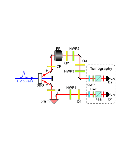
Figure 1: (Color online). Experimental setup. Maximally entangled polarization photon pairs, created from the spontaneous parametric down conversion process by pumping the two-crystal geometry type I BBO with ultraviolet (UV) pulses, are emitted into paths $a$ and $b$. These two photons pass through quartz plates (CP) to compensate the birefringence in BBO. A half-wave plate (HWP1) and quartz plates (Q1) in path $a$ are used to prepared the required mixed state. The Fabry-Perot (FP) cavity together with quartz plates (Q2 and Q3) and two half-wave plates (HWP2 and HWP3) in path $b$ is employed to monitor the dephasing coupling. After passing through quarter-wave plates (QWP), half-wave plates (HWP) and polarization beam splitters (PBS) which allow to tomographically reconstruct the density matrix, both photons are then registered by single-photon detectors (D1 and D2) equipped with 3 nm interference filters (IF).

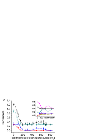
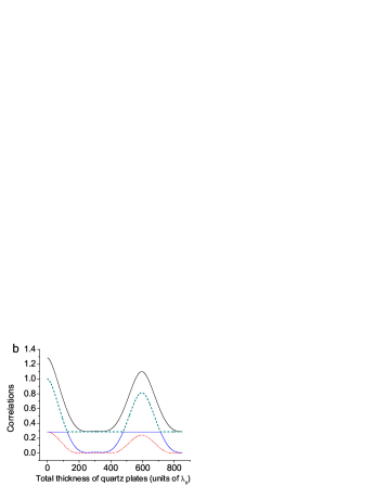
Figure 2: (Color online). (a) Experimental results of the non-Markovian dynamics of correlations. Black squares, dark cyan diamonds, blue stars and red dots represent the experimental results of $\mathcal{I}$, $\mathcal{C}$, $\mathcal{Q}$ and $REE$ with the black solid line, dark cyan dashed line, blue solid line and red dotted line representing the corresponding theoretical prediction, respectively. The inset (the $x$ axes represent the total thickness of Q2) represents the corresponding evolution of eigenvalues of $\rho$ and $\chi_{\rho}$. The magenta, dark cyan, blue and dark yellow dots represent the experimental results of $\lambda_{1}$, $\lambda_{2}$, $\lambda_{3}$ and $\lambda_{4}$ with the magenta, dark cyan, blue and dark yellow solid lines representing the corresponding theoretical predictions, respectively. Black squares and red stars represent the experimental results of $\frac{1}{2}(\lambda_{1}+\lambda_{2})$ and $\frac{1}{2}(\lambda_{3}+\lambda_{4})$ with the black and red solid lines representing the corresponding theoretical predictions, respectively. (b) Theoretical predictions of the correlation dynamics with the FWHM of $f(\omega_{b})$ identically fitting to 0.2 nm. The black solid line, dark cyan dashed line, blue solid line and red dotted line represent $\mathcal{I}$, $\mathcal{C}$, $\mathcal{Q}$ and $REE$, respectively. $\lambda_{0}=0.78$ $\mu$m.

In our experiment, the final output state is a Bell diagonal state with the form of equation (7). According to the equal footing method Modi10 , experimental results of quantum correlation ($\mathcal{Q}$), classical correlation ($\mathcal{C}$) and total correlation ($\mathcal{I}$) are deduced from equations (1), (2) and (3) with $S(\pi_{\chi_{\rho}})=S(\pi_{\rho})$, respectively. The relative entropy of entanglement ($REE$) can be calculated from the maximal eigenvalue of $\rho$ according to equations (4) and (5) Vedral97 . As a result, all kinds of correlations can be deduced from the density matrix of $\rho$.

Fig. 2 displays the dynamics of correlations, as a function of the thickness of Q2 which is represented by the corresponding retardation $x$ ($L=x/\Delta n$). The thickness of Q1 represented by the retardation is set to be $117\lambda_{0}$ ($\lambda_{0}$=0.78 $\mu$m is the central wavelength of the photon) to prepare the initial mixed state and $\kappa_{a}$ is equal to about 0.607. The HWP2 and HWP3 are not used (i. e., without $\sigma_{x}$ operation) and Q3 is set to 0, in which the phenomenon of entanglement collapse and revival occurs Xu102 . We find that there exhibits a sudden transition from classical to quantum decoherence area Xu10 ; Mazzola10 . At the beginning of the evolution, the quantum correlation $\mathcal{Q}$ (blue stars) remains constant and then decays exponentially after the thickness of about $120\lambda_{0}$. Due to the refocusing effect of the relative phase, $\mathcal{Q}$ revives from near zero at the thickness of about $440\lambda_{0}$ and reaches the maximum of 0.11 at about $540\lambda_{0}$. With further increasing Q2, $\mathcal{Q}$ decays monotonically again. The classical correlation $\mathcal{C}$ (dark cyan diamonds) behaviors quite differently. It decays exponentially at the beginning and then remains constant all the time after the thickness of $120\lambda_{0}$ despite the non-Markovian effect. $\mathcal{Q}$ and $\mathcal{C}$ overlap at the thickness of $120\lambda_{0}$, in which the sudden change in behavior in their decay rates are observed Maziero09 ; Xu10 . The evolution of relative entropy of entanglement $REE$ (red dots) is also shown, which suffers from sudden death Yu09 at the thickness of about $189\lambda_{0}$ and is consistent with our previous results Xu102 . If we continue to increase Q2, $REE$ also revives to its maximally value at the thickness of about $540\lambda_{0}$ (the value is relative small in the figure). The evolution of total correlation $\mathcal{I}$ (black squares) first decays exponentially and then revives just as that of $\mathcal{Q}$. The black solid line, dark cyan dashed line, blue solid line and red dotted line represent the theoretical predictions of $\mathcal{I}$, $\mathcal{C}$, $\mathcal{Q}$ and $REE$. The inset displays the corresponding dynamics of eigenvalues of $\rho$ and $\chi_{\rho}$. The magenta, dark cyan, blue and dark yellow dots represent the experimental results of $\lambda_{1}$, $\lambda_{2}$, $\lambda_{3}$ and $\lambda_{4}$ with the magenta, dark cyan, blue and dark yellow solid lines representing the corresponding theoretical predictions, respectively. Whereas the black squares and red stars represent the experimental results of $\frac{1}{2}(\lambda_{1}+\lambda_{2})$ and $\frac{1}{2}(\lambda_{3}+\lambda_{4})$ with the black and red solid lines representing the corresponding theoretical predictions. It can be seen clearly that the sudden transition of classical and quantum decoherence occurs at the point when the switch in the second maximal eigenvalue $\lambda_{2}$ occurs Mazzola10 and it is consistent with our previous theoretical prediction. At the period with the relative phase refocusing, the four eigenvalues $\lambda_{i}$ behave correspondingly, i. e., $\lambda_{1}$ ($\lambda_{3}$) increases and $\lambda_{2}$ ($\lambda_{4}$) decreases. However, $\frac{1}{2}(\lambda_{1}+\lambda_{2})$ and $\frac{1}{2}(\lambda_{3}+\lambda_{4})$ remain constant and there is not revival of $\mathcal{C}$ according to its definition. The errors of the experimental results are estimated using the method proposed in ref. James01 , which is mainly due to the random fluctuation of each measured coincidence counts (the errors from the uncertainties in aligning the wave plates is relatively small). In this approach, the errors are directly deduced from the fluctuation of the corresponding eigenvalues. The error bars of the relative entropy of entanglement involve only the maximal eigenvalue of $\rho$, which are relative small in the figure.

In our experiment, the frequency distribution $f(\omega_{b})$ is treated as three Gauss-like wave packets centered at 778.853, 780.160 and 781.459 nm with the relative probabilities of 0.37, 0.44 and 0.19, respectively Xu102 . The FWHM of these wave packets are identically considered as 0.85 nm and we obtain good fittings. The maximal revival value of $\kappa_{b}$ is about 0.385, which is smaller than $\kappa_{a}$. As a result, the classical correlation remains constant after the sudden transition point in the case of Fig. 2a, which is immune from the non-Markovian effect and is consistent with our previous analysis in the theoretical part. With the narrower FWHM of $f(\omega_{b})$, the maximal revival value of $\kappa_{b}$ can be larger than $\kappa_{a}$ and the switch in the second maximal eigenvalue would occur again, in which the refocusing effect would be strong enough to revive the classical correlation. Fig. 2b shows the theoretical prediction of the correlation dynamics with the FWHM of $f(\omega_{b})$ identically fitting to 0.2 nm (the maximal revival value of $\kappa_{b}$ is about 0.944). We can see that $\mathcal{I}$ (black solid line), $\mathcal{C}$ (dark cyan dashed line), $\mathcal{Q}$ ( blue solid line) and $REE$ (red dotted line) are all revived. The sudden transition from quantum to classical revival regime is obtained at the thickness of about $477\lambda_{0}$ (the revival value of $\kappa_{b}$ is equal to $\kappa_{a}$).

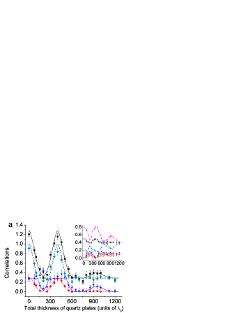
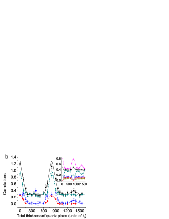
Figure 3: (Color online). Experimental results of correlation echoes: (a) with the $\sigma_{x}$ operation at $200\lambda_{0}$; (b) with the $\sigma_{x}$ operation at $400\lambda_{0}$. Black squares, dark cyan diamonds, blue stars and red dots represent the experimental results of $\mathcal{I}$, $\mathcal{C}$, $\mathcal{Q}$ and $REE$ with the black solid line, dark cyan dashed line, blue solid line and red dotted line representing the corresponding theoretical predictions, respectively. The $x$ axes represent the total thickness of Q2 and Q3. The blue arrows identify the $\sigma_{x}$ operation points. The insets in (a) and (b) (the $x$ axes represent the total thickness of Q2 and Q3) represent the corresponding evolution of eigenvalues of $\rho$ and $\chi_{\rho}$, respectively. The magenta, dark cyan, blue and dark yellow dots represent the experimental results of $\lambda_{1}$, $\lambda_{2}$, $\lambda_{3}$ and $\lambda_{4}$ with the magenta, dark cyan, blue and dark yellow solid lines representing the corresponding theoretical predictions, respectively. Black squares and red stars represent the experimental results of $\frac{1}{2}(\lambda_{1}+\lambda_{2})$ and $\frac{1}{2}(\lambda_{3}+\lambda_{4})$ with the black and red solid lines representing the corresponding theoretical predictions, respectively. $\lambda_{0}=0.78$ $\mu$m.

It is a great challenge to realize the small FWHM to obtain the observable revival of classical correlation in the experiment. We then implement a $\sigma_{x}$ operation on the photon in path $b$ to investigate the correlation dynamics and get the revival of classical correlation. The thickness of Q2 is first increased to $200\lambda_{0}$ or $400\lambda_{0}$ followed by a $\sigma_{x}$ operation which is fulfilled by the HWP2. The thickness of Q3 is then increased from zero without further increase of Q2 to get the corresponding dynamics of correlations, which are shown in Fig. 3a (Q2=200$\lambda_{0}$) and Fig. 3b (Q2=$400\lambda_{0}$), respectively (the $x$ axes represent the total thickness of Q2 and Q3). The black squares, dark cyan diamonds, blue stars and red dots represent the experimental results of $\mathcal{I}$, $\mathcal{C}$, $\mathcal{Q}$ and $REE$ with the black solid line, dark cyan dashed line, blue solid line and red dotted line representing the corresponding theoretical predictions, respectively. We can see that correlation echoes are formed when Q3=$200\lambda_{0}$ in Fig. 3a and Q3=$400\lambda_{0}$ in Fig. 3b, i. e., at the time when Q3 is increased to the same thickness as Q2. This implies that the dephasing effect between $|H\rangle$ and $|V\rangle$ caused by Q2 is completely compensated by Q3 and all the correlations maximally revives to the initial values. During this process, the sudden transition from quantum to classical revival area is observed (Fig. 3a at the thickness of about $280\lambda_{0}$ and Fig. 3b at the thickness of about $680\lambda_{0}$). The classical correlation revives from the constant period to its maximal value, whereas the quantum correlation stops revival and remains constant. If we further increase Q3, the subsequent dynamics of correlations are just the same as that shown in Fig. 2a. The blue arrows in the figures identify the $\sigma_{x}$ operation points. The correlation dynamics between the initial state and the maximally revived states are symmetric about the $\sigma_{x}$ operation point, which is similar to the phenomenon of spin echo in nuclear magnetic resonance Hahn50 . The insets in Fig. 3a and Fig. 3b represent the corresponding dynamics of eigenvalues of $\rho$ and $\chi_{\rho}$. The magenta, dark cyan, blue and dark yellow dots represent the experimental results of $\lambda_{1}$, $\lambda_{2}$, $\lambda_{3}$ and $\lambda_{4}$ with the magenta, dark cyan, blue and dark yellow solid lines representing the corresponding theoretical predictions, respectively. Whereas the black squares and red stars represent the experimental results of $\frac{1}{2}(\lambda_{1}+\lambda_{2})$ and $\frac{1}{2}(\lambda_{3}+\lambda_{4})$ with the black and red solid lines representing the corresponding theoretical predictions, respectively. We can see that the eigenvalues also display the echo effect and the second switch in the second maximal eigenvalue $\lambda_{2}$ in both the insets of Fig. 3a and 3b leads to the revival of classical correlation.

IV Discussion and Conclusion

The reasons for quantum advantage in quantum information processing are still controversial Vedral09 . Recently, a simple one-to-one relationship between bipartite entanglement of formation Bennett96 and quantum discord in a general tripartite system is proposed Fanchini102 . By taking the environment which is initially maximally entangled to the system with the reduced maximally mixed state in the DQC1 protocol into consideration, it is suggested that both the quantum discord and entanglement are responsible for the quantum computer speedup Fanchini102 . Inspired by the factorization law of entanglement evolution in noisy quantum channels Konrad08 ; Farias09 ; Xu09 , it is expected that similar simple relationship for quantum correlation under noise environment exists. With the increasing interests, there will be more distinctive discoveries in this field.

In our experiment, we have investigated the correlation dynamics in a non-Markovian dephasing environment. The whole point of a non-Markovian environment is that it retains a memory of a system at a given time and then later passes this information back into the system in some form or another. In this experiment, the non-Markovian environment acts via the FP cavity followed by quartz plates on the biphoton system of only one of the photons. Due to the discrete frequency distribution of the photon which leads to the refocusing of the relative phase in the dephasing environment, the non-Markovian effect occurs and the revival of quantum correlation is obtained from near zero area. However, the non-Markovian effect is too weak to revive the classical correlation. With the narrower FWHM of the wave packets of the discrete frequency distribution, the revival of classical correlation would be also achieved. On the other hand, if the FWHM of the wave packets become lager, the non-Markovian effect becomes weaker. When the discrete frequency distribution tends to continuous Gaussian distribution, we would get the Markovian limited dynamics. We further implement a $\sigma_{x}$ operation on the photon in path $b$ to investigate the corresponding correlation dynamics. During this process, we obtain correlation echoes, in which the sudden transition from quantum to classical revival regime is observed. This work is a useful and informative add-on to our previous works, in which the entanglement collapse and revival is observed Xu102 and the Markovian limited dynamics of correlations is demonstrated Xu10 . The method can be used to control the revival time of correlations, which would find important applications in quantum memory.

We thank Cheng-Hao Shi for help in performing the experiment. This work was supported by National Fundamental Research Program, National Natural Science Foundation of China (Grant Nos. 60921091, 10734060, 10874162, 11004185), China Postdoctoral Science Foundation (Grant No. 20100470836) .

References

- (1) M. A. Nielsen and I. L. Chuang, Quantum Computation and Quantum Information (Cambridge University Press, Cambridge, England, 2000).
- (2) H. Ollivier and W. H. Zurek, Phys. Rev. Lett. 88, 017901 (2001).
- (3) L. Henderson and V. Vedral, J. Phys. A: Math. Gen. 34, 6899 (2001).
- (4) A. Datta, A. Shaji, and C. M. Caves, Phys. Rev. Lett. 100, 050502 (2008).
- (5) B. P. Lanyon, M. Barbieri, M. P. Almeida, and A. G. White, Phys. Rev. Lett. 101, 200501 (2008).
- (6) C. E. Shannon, Bell Syst. Tech. J. 27, 379 (1948).
- (7) B. Groisman, S. Popescu, and A. Winter, Phys. Rev. A 72, 032317 (2005).
- (8) A. Ferraro, L. Aolita, D. Cavalcanti, F. M. Cucchietti, and A. Acin, Phys. Rev. A 81, 052318 (2010).
- (9) M. S. Sarandy, Phys. Rev. A 80, 022108 (2009).
- (10) T. Werlang and G. Rigolin, Phys. Rev. A 81, 044101 (2010).
- (11) Y.-X. Chen and S.-W. Li, Phys. Rev. A 81, 032120 (2010).
- (12) T. Werlang, C. Trippe, G. A. P. Ribeiro, and G. Rigolin, Phys. Rev. Lett. 105, 095702 (2010).
- (13) J. H. Cole, J. Phys. A: Math. Theor. 43, 135301 (2010).
- (14) R.-C. Ge, M. Gong, C.-F. Li, J.-S. Xu, and G.-C. Guo, Phys. Rev. A 81, 064103 (2010).
- (15) J.-S. Xu, et al., Nat. Commun. 1, 7 (2010).
- (16) F. F. Fanchini, L. K. Castelano, and A. O. Calderia, New J. Phys. 12, 073009 (2010).
- (17) D. O. Soares-Pinto et al., Phys. Rev. A 81, 062118 (2010).
- (18) P. Giorda and M. G. A. Paris, Phys. Rev. Lett. 105, 020503 (2010).
- (19) G. Adesso and A. Datta, Phys. Rev. Lett. 105, 030501 (2010).
- (20) R. Vasile, P. Giorda, S. Olivares, M. G. A. Paris and S. Maniscalco, Phys. Rev. A 82, 012313 (2010).
- (21) K. Bradler, M. M. Wilde, S. Vinjanampathy and D. B. Uskov, arXiv:0912.5112 (2010).
- (22) A. Shabani and D. A. Lidar, Phys. Rev. Lett. 102, 100402 (2009).
- (23) W. H. Zurek, Phys. Rev. A 67, 012320 (2003).
- (24) A. Datta, Phys. Rev. A 80, 052304 (2009).
- (25) J.-C. Wang, J.-F. Deng, and J.-L. Jing, Phys. Rev. A 81, 052120 (2010).
- (26) B. M. Terhal, M. Horodecki, D. W. Leung, and D. P. DiVincenzo, J. Math. Phys. 43, 4286 (2002).
- (27) D. P. DiVincenzo, M. Horodecki, D. W. Leung, J. A. Smolin, and B. M. Terhal, Phys. Rev. Lett. 92, 067902 (2004).
- (28) J. Oppenheim, M. Horodecki, P. Horodecki, and R. Horodecki, Phys. Rev. Lett. 89, 180402 (2002).
- (29) M. Horodecki, et al., Phys. Rev. A 71, 062307 (2005).
- (30) S. Luo, Phys. Rev. A 77, 022301 (2008).
- (31) K. Modi, T. Paterek, W. Son, V. Vedral, and M. Williamson, Phys. Rev. Lett. 104, 080501 (2010).
- (32) T. Yu and J. H. Eberly, Science 323, 598 (2009).
- (33) T. Werlang, S. Souza, F. F. Fanchini, and C. J. Villas Boas, Phys. Rev. A 80, 024103 (2009).
- (34) J. Maziero, L. C. Céleri, R. M. Serra, and V. Vedral, Phys. Rev. A 80, 044102 (2009).
- (35) L. Mazzola, J. Piilo, and S. Maniscalco, Phys. Rev. Lett. 104, 200401 (2010).
- (36) B. Wang, Z.-Y. Xu, Z.-Q. Chen, and M. Feng, Phys. Rev. A 81, 014101 (2010).
- (37) F. F. Fanchini, T. Werlang, C. A. Brasil, L. G. E. Arruda, and A. O. Caldeira, Phys. Rev. A 81, 052107 (2010).
- (38) V. Vedral, M. B. Plenio, M. A. Rippin, and P. L. Knight, Phys. Rev. Lett. 78, 2275 (1997).
- (39) A. J. Berglund, arXiv:quant-ph/0010001 (2000).
- (40) J.-S. Xu et al., Phys. Rev. Lett. 104, 100502 (2010).
- (41) E. Hahn, Phys. Rev. 80, 580 (1950).
- (42) P. G. Kwiat, E. Waks, A. G. White, I. Appelbaum, and P. H. Eberhard, Phys. Rev. A 60, R773 (1999).
- (43) J.-S. Xu, C.-F. Li, and G.-C. Guo, Phys. Rev. A 74, 052311 (2006).
- (44) D. F. V. James, P. G. Kwiat, W. J. Munro, and A. G. White, Phys. Rev. A 64, 052312 (2001).
- (45) V. Vedral, arXiv:0906.3656 (2009).
- (46) C. H. Bennett, D. P. DiVincenzo, J. A. Smolin, and W. K. Wootters, Phys. Rev. A 54, 3824 (1996).
- (47) F. F. Fanchini, M. F. Cornelio, M. C. de Oliveira, and A. O. Caldeira, arXiv:1006.2460 (2010).
- (48) T. Konrad, et al. Nat. Phys. 4, 99 (2008).
- (49) O. J. Farias, et al. Science 323, 1414 (2009).
- (50) J.-S. Xu, et al. Phys. Rev. Lett. 103, 240502 (2009).