Global Modeling and Prediction of Computer Network Traffic

Abstract

We develop a probabilistic framework for global modeling of the traffic over a computer network. This model integrates existing single–link (–flow) traffic models with the routing over the network to capture the global traffic behavior. It arises from a limit approximation of the traffic fluctuations as the time–scale and the number of users sharing the network grow. The resulting probability model is comprised of a Gaussian and/or a stable, infinite variance components. They can be succinctly described and handled by certain ’space–time’ random fields. The model is validated against simulated and real data. It is then applied to predict traffic fluctuations over unobserved links from a limited set of observed links. Further, applications to anomaly detection and network management are briefly discussed.

1 Introduction

Understanding the statistical behavior of computer network traffic has been an important and challenging problem for the past 15 years, because of its impact on network performance and provisioning [21, 29, 15, 26] and on the potential for development of more suitable protocols [25, 26]. Since the early 1990s it has been well established that the traffic over a single link exhibits intricate temporal dependence, known as burstiness, which could not be explained by traffic models developed for telephone networks [20]. This phenomenon could be understood and described by using the notions of long–range dependence and self–similarity [12], which in turn are affected by the presence of heavy tails in the distribution of file sizes [7, 25]. A bottom-up mechanistic model for single link network traffic that is in agreement with the empirical features observed in real network traces was presented in [38]. A competing model based on queuing ideas was studied in [22]. These works lead to many further developments (see eg [26]).

Advances in technology that allowed the acquisition of direct, through sampling [10, 42], and indirect [19] measurements have allowed researchers to examine the characteristics of traffic in entire networks [18, 15, 31, 41], based on statistical modeling analysis. On the other hand, an analogue of the mechanistic models available for single link network traffic is not available. Such a model would allow better understanding of network performance [13, 21] and detection of anomalous behavior [27]. Further, it would manage to capture and explain statistical relationships between flows traversing the network at all time scales (time) and across all links (space); the latter represents a fairly tall requirement, which may also prove rather impractical given the underlying complexity (protocols, applications) and heterogeneity (physical infrastructure, diverse users) of modern networks.

Our objective in this paper is to propose a mechanistic model that captures several fundamental characteristics of network-wide traffic and thus constitutes a partial solution for this challenging problem. The model is based on modeling user behavior on source–destination paths across the network and then aggregate over users and over time, thus developing a joint ’space–time’ probability model for the traffic fluctuations over all links in the network. This model reflects the statistical dependence of the traffic across different links, observed at the same or different points in time. We demonstrate the success of our modeling strategy in the context of network traffic prediction – a problem with important implications on network performance, provisioning, and management.

The remainder of the paper is structured as follows. In Section 2.1, we review briefly the existing and relatively well–understood theory of single–flow (link) models for the temporal dependence in network traffic. Long–range dependence and heavy tails play a central role. In Section 3, we postulate our network–wide model based on combining single–flow models through the routing equation. We show that the scaling limit of such a model is a combination of fractional Brownian motions and infinite variance stable Lévy motions. A succinct representation of these processes is given in Section 3.2 via the functional fractional Brownian motion and functional Lévy stable motion. The resulting model is then used in Section 4 to solve the network kriging problem, i.e. to predict the traffic fluctuations on a unobserved link from a limited set of measurements of observed links. In Section 5, we use extensive NetFlow data of sampled network traffic to obtain approximations of the flow–level traffic $X_{j}(t)$. These data are then used to validate our model and demonstrate the success of the network kriging methodology. We conclude in Section 6 with some remarks on future applications, statistical problems on networks, and further extensions of the network–wide probabilistic model.

2 Problem Formulation

Consider a computer network of $L$ links and $N$ nodes. The network typically carries traffic flows (via groups of packets) from any node (source) to any other node (destination) over a predetermined set of links (route). This can be formally described by the routing matrix $A=(a_{\ell j})_{L\times{\cal J}}$, where

$$a_{\ell j}=\left\{\begin{array}[]{ll}1&,\ \mbox{ {\em route} $j$ involves {\em link} $\ell$ }\\ 0&,\ \mbox{ otherwise,}\end{array}\right.$$

and where ${\cal J}$ is the total number of routes (typically, ${\cal J}=N(N-1)$).

We describe next the physical premises of our modeling framework. We assume, for simplicity, that the traffic is fluid. That is, the amount of data (bytes) transmitted over link $\ell$ during the time interval $(a,b)$ is $\int_{a}^{b}Y_{\ell}(t)dt$, where $Y_{\ell}(t)$ is the traffic intensity (bytes per unit time) over link $\ell$. Let also $X_{j}(t)$ denote the traffic intensity at time $t$ over route $j,\ 1\leq j\leq{\cal J}$. Then, assuming that traffic propagates instantaneously over the network, we obtain the following routing equation:

$$\vec{Y}(t)=A\vec{X}(t),$$ (1)

where $\vec{X}(t)=(X_{j}(t))_{1\leq j\leq{\cal J}}$ and $\vec{Y}(t)=(Y_{\ell}(t))_{1\leq\ell\leq L}$. This relationship is valid only to the extent that traffic propagates instantaneously along the routes. Thus, (1) cannot be adopted over the finest, high–frequency time scales where packet delay plays a central role. On the other hand, for all practical purposes, the routing equation holds over a wide range of time scales greater than the RTT (round trip time) for packets in the network [31, 42]. This equation captures the fundamental relationship between the traffic intensity over different routes in the network and the resulting load, incurred on the links.

From a physical perspective, the computer network is merely used to ’transport’ information from source nodes to destination nodes. In normal (uncongested) operating regime, the traffic is carried seamlessly and the traffic intensities $X_{j}(t)$ are driven solely by the demand along the routes $j,\ 1\leq j\leq{\cal J}.$ Thus, as a first approximation one may view the $X_{j}(t)$’s as statistically independent in $j,\ 1\leq j\leq{\cal J}$. Therefore, in view of (1), the statistical dependence between $Y_{\ell_{1}}(t)$ and $Y_{\ell_{2}}(t)$ for two links $\ell_{1}$ and $\ell_{2}$, is governed by the set of routes $X_{j}(t)$ that use both $\ell_{1}$ and $\ell_{2}$.

In view of the above discussion, guided by the routing equation (1), we obtain a global model for the traffic intensity $Y_{\ell}(t),\ 1\leq\ell\leq L,\ t\geq 0$. The temporal dependence of the flow–level traffic $X_{j}(t)$ can be described well by the existing mechanistic models exhibiting long–range dependence and heavy tails (see Section 2.1). The independence of the $X_{j}(t)$’s in $j$ is a questionable assumption when the network is not in equilibrium or it is congested. Indeed, if two routes share a congested node, then the feedback mechanism of TCP clearly induces dependence between the two flows. Further, since every TCP session involves ACK (acknowledgment) packets traversing along the reverse route, then in practice one expects dependence between the forward and reverse flows for a given pair of a source and destination. Our experience with NetFlow data for the Internet2 backbone network suggests however that for the present utilization levels of the network (about 10% to 20%) the $X_{j}(t)$’s are nearly uncorrelated in $j$ (see Fig. 2 in Section 5). The correlation is strongest but still rather weak among the forward and reverse flows (see also [31]).

Therefore, as a first attempt to model globally the dependence structure of the network across all links and in time, we advocate adopting the simple assumption of independence of the flow–level traffic. Our methodology can be extended to cover more complex scenarios of dependence between forward and reverse flows, as well as ’second–order’ effects of dependence between flows triggered by congestion. This should be done with caution however since the chaotic behavior induced by the TCP feedback is not well–understood on network–wide level.

2.1 A Brief Overview of Single Link Traffic Models

We start with a brief review of single–link traffic models, since a number of their features are incorporated into our network–wide model. Such models are built on the paradigm of multiple users sharing a link. Depending on the regimes prevalent in the network, one obtains two qualitatively different asymptotic models for the cumulative traffic fluctuations. One regime leads to finite–variance, Gaussian models that exhibit long–range dependence and self–similarity. The other regime yields infinite variance processes with independent increments.

2.2 Activity rate models: two limit regimes

Consider a fixed route on the network and suppose that $M$ independent users share this route. Let $\{X(t)\}_{t\geq 0}$ denote the traffic intensity of one such user in bytes per unit time. Thus $\int_{a}^{b}X(t)dt$ is the total traffic (bytes) generated by the user during the time interval $(a,b)$. It is assumed that $\{X(t)\}_{t\geq 0}$ is a strictly stationary stochastic process with finite mean.

Following the framework in [24], let $\{(T_{j},Z_{j})\}_{j\in{\mathbb{Z}}}$ be a stationary marked point process of arrival times $T_{j}$’s in ${\mathbb{R}}$ with marks $Z_{j}$’s. At time $T_{j}$, the user initiates a transmission at constant unit rate, which lasts time $Z_{j}$. Thus, the traffic intensity at time $t$ equals:

$$X(t)=\sum_{j\in{\mathbb{Z}}}I(T_{j}\leq t<T_{j}+Z_{j}),$$ (2)

where $\cdots\leq T_{0}\leq 0\leq T_{1}\leq\cdots$. One can recover the following two popular traffic models as special cases:

• $M/G/\infty$ model: If the $T_{j}$’s are arrival times of a Poisson point process with constant intensity, independent of the marks $Z_{j}$’s, then $\{X(t)\}_{t\geq 0}$ becomes the $M/G/\infty$ model.

• On/Off model: On the other hand, if the $Z_{j}$’s and the $T_{j}$’s are dependent and such that:

  $$T_{j,{\rm on}}:=T_{j},\ \ T_{j,{\rm off}}:=T_{j}+Z_{j}<T_{j+1}\equiv T_{j+1,{\rm on}},$$

  then $X(t)$ follows the On/Off model, i.e. a period of activity (’On’) is followed by an idle period (’Off’). It is further assumed that the On periods: $U_{j,{\rm on}}:=Z_{j}$ and the Off periods $U_{j,{\rm off}}:=T_{j+1}-T_{j}+Z_{j}$, are mutually independent and identically distributed with laws $F_{\rm on}(x)={\mathbb{P}}\{U_{1,{\rm on}}\leq x\}$ and $F_{\rm off}(x)={\mathbb{P}}\{U_{1,{\rm off}}\leq x\}$.

Remark. The initial On period $T_{1,\rm on}$ has such a distribution as to ensure that $\{X(t)\}$ is stationary. This can happen only if the On and Off periods have finite means. The work [23] addresses the case of activity rates with very heavy tails, which can have infinite means.

In the context of network traffic, the durations of the user activity $Z_{j}$’s are modeled with heavy tailed distributions with finite mean but infinite variance, since they can be linked to the ubiquitous presence of heavy tails in computer networks (file sizes, web pages, etc. see e.g. [7, 25, 8]). The heavy tailed nature of the durations, implies that the process $X(t)$ of user activity is long–range dependent (LRD). The intimate connection between the long–range dependence phenomenon and self–similarity provides an appealing mechanistic (physical) explanation of the cause of burstiness in network traffic (see e.g. [20, 12, 40], [26] and the references therein).

For brevity, we focus on the On/Off model and suppose that the tails of the On and Off durations are heavy, i.e. as $x\to\infty$:

$$1-F_{\rm on}(x):=\overline{F}_{\rm on}(x)\sim c_{\rm on}x^{-\alpha_{\rm on}}\ \mbox{ and }\ \overline{F}_{\rm Off}(x)=c_{\rm off}x^{-\alpha_{\rm off}},$$

for some constants $c_{\rm on},\ c_{\rm off}>0$ and tail exponents, such that

$$1<\alpha:=\min\{\alpha_{\rm on},\alpha_{\rm off}\}<2.$$ (3)

Relation (3) then implies that $X(t)$ is LRD with Hurst exponent

$$H=\frac{3-\alpha}{2}\in(1/2,1),$$ (4)

that is, for some constant $c_{X}>0$,

$${\rm Cov}(X(t),X(0))\sim c_{X}t^{2H-2},\ \ \mbox{ as }t\to\infty$$

(see e.g. [24]).

2.3 Multiple Sources Asymptotics: Long–Range Dependence and Heavy Tails

Let now $\{X^{(i)}(t)\}$, $1\leq i\leq M$ be independent and identically distributed stationary processes modeling the traffic intensities of $M$ users sharing a given route. Then, the cumulative traffic over the route generated by the users is:

$$X^{*}(T,M):=\int_{0}^{T}\sum_{i=1}^{M}X^{(i)}(t)dt.$$

We are interested in the asymptotic behavior of the cumulative traffic fluctuations about the mean:

$$X_{0}^{*}(T,M):=X^{*}(T,M)-{\mathbb{E}}X^{*}(T,M).$$

As shown in the seminal work of [38], if the $X^{(i)}(t)$’s are On/Off processes, then

$${\cal L}\lim_{T\to\infty}\frac{1}{T^{H}}{\Big{\{}}{\cal L}\lim_{M\to\infty}\frac{1}{\sqrt{M}}X_{0}^{*}(Tt,M){\Big{\}}}_{t\geq 0}=\{B_{H}(t)\}_{t\geq 0},$$ (5)

where $B_{H}=\{B_{H}(t)\}_{t\geq 0}$ is a fractional Brownian motion (fBm) with self–similarity parameter $H$ as in (4) and where ’${\cal L}\lim$’ denotes finite–dimensional distributions convergence. Recall that the fBm $B_{H}$ is a zero mean Gaussian process with stationary increments, which is self–similar, i.e. for all $c>0$, we have $\{B_{H}(ct)\}_{t\geq 0}\stackrel{{\scriptstyle d}}{{=}}\{c^{H}B_{H}(t)\}_{t\geq 0}$. One necessarily has that $H\in(0,1)$ and, for some $\sigma^{2}={\rm Var}(B_{H}(1))>0$:

$${\rm Cov}(B_{H}(t),B_{H}(s))=\frac{\sigma^{2}}{2}{\Big{(}}|t|^{2H}+|s|^{2H}-|t-s|^{2H}{\Big{)}},\ t,s\geq 0$$

(see e.g. [30]).

Relation (5) shows that the fluctuations of the cumulative traffic about its mean behave asymptotically like the fractional Brownian motion, as the number of users $M$ and the time scale $T$ are sufficiently large. The increments $G(k):=B_{H}(k)-B_{H}(k-1),\ k=1,2,\dots,$ of fBm then can then serve as a model for the traffic traces of the number of bytes transmitted over the network over certain, sufficiently large time scales.

The order of the limits in (5) is important. If one takes $T\to\infty$ first and then $M\to\infty$, as shown in [38], one obtains:

$${\cal L}\lim_{M\to\infty}\frac{1}{M^{1/\alpha}}{\Big{\{}}{\cal L}\lim_{T\to\infty}\frac{1}{T^{1/\alpha}}X_{0}^{*}(Tt),M{\Big{\}}}_{t\geq 0}=\{\Lambda_{\alpha}(t)\}_{t\geq 0}.$$ (6)

Now the limit process $\Lambda_{\alpha}=\{\Lambda_{\alpha}(t)\}_{t\geq 0}$ has independent and stationary increments with $\alpha-$stable distributions, with $\alpha$ being as in (3). It is the Lévy stable motion – the infinite variance counterpart to the Brownian motion.

Relations (5) and (6) show two different regimes for the network. The first involves many users relative to the time scale and the second, just a few users relative to the time scale. As shown in [22] (see also [14, 28, 24]), one can consider the limit when the number of users $M=M(T)$ grows to infinity, as a function of the time scale $T$. Then:

• (fast growth) If ${(M(T)T)^{1/\alpha}}/{T}\to\infty,$ as $T\to\infty$, then

  $${\cal L}\lim_{T\to\infty}{\Big{\{}}\frac{1}{T^{H}\sqrt{M(T)}}X_{0}^{*}(Tt,M){\Big{\}}}_{t\geq 0}=\{B_{H}(t)\}_{t\geq 0}.$$

• (slow growth) If ${(M(T)T)^{1/\alpha}}/{T}\to 0,$ as $T\to\infty$, then

  $${\cal L}\lim_{T\to\infty}{\Big{\{}}\frac{1}{(TM(T))^{1/\alpha}}X_{0}^{*}(Tt,M){\Big{\}}}_{t\geq 0}=\{\Lambda_{\alpha}(t)\}_{t\geq 0}.$$

The fast growth scenario shows that if the number of users $M(T)$ grows relatively fast, then the same limit as in (5) is achieved. The slow growth regime on the other hand, yields the stable Lévy motion in the limit, when there are relatively few users sharing the link. The intermediate regime when ${(M(T)T)^{1/\alpha}}/{T}\to c\in(0,\infty)$ is considered in [14].

This abundant theory offers a multitude of tools for modeling the temporal dependence of traffic traces in various regimes. For example, the users need not be of the same type. As in [9] one may consider $q$ classes of users $M_{k},\ 1\leq k\leq q$, where $M=\sum_{k=1}^{q}M_{k}$, and $M_{k}(T)\to\infty$ as $T\to\infty.$ The users within a given class are of the same type with parameters $\alpha_{k}\in(1,2),$ and $H_{k}:=(3-\alpha_{k})/2,\ 1\leq k\leq q$. By balancing the rates of the $M_{k}(T)$’s one can obtain in the limit

$${\cal L}\lim_{T\to\infty}\{\frac{1}{a(T)}X_{0}^{*}(Tt,M)\}_{t\geq 0}=\sum_{k\in{\cal F}}B_{H_{k}}+\sum_{k\in{\cal S}}\Lambda_{\alpha_{k}},$$

where $B_{H_{k}}=\{B_{H_{k}}(t)\}_{t\geq 0}$ and $\Lambda_{\alpha_{k}}=\{\Lambda_{\alpha_{k}}(t)\}_{t\geq 0},\ 1\leq k\leq q$ are independent fBm’s and Lévy stable motions, respectively. Here $\{1,\cdots,q\}={\cal F}\cup{\cal S}$ is the partition of the groups of users into subsets of fast and slow growth regimes, respectively.

Similar results were shown to hold for the $M/G/\infty$ and other activity rate models (see e.g. [24]). Remarks.

1. If the individual user behavior is modeled by $M/G/\infty$ processes with heavy–tailed, infinite variance durations $Z_{j}$’s, then similar asymptotic results hold for the cumulative traffic fluctuations. In fact, as shown in [24], this is so for the general activity rate model in (2).

2. As argued above, by balancing the rates of multiple groups of users, one can obtain complex hybrid models, composed of fBm’s and Lévy stable motions. In practice, however, typically one component dominates. In fact, as shown in [24], the fBm limit is more robust than the Lévy stable motion with respect to the type and the regimes of the activity rate models considered.

   In fact, the fundamental theorem of Lamperti (see eg Theorem 2.1.1 in [11]) implies an interesting robustness and homogeneity property. Namely, suppose that $X^{(i)}(t)$’s are all stationary in $t$. If the the time–scale limit

   $${\cal L}\lim_{T\to\infty}\{\frac{1}{a(T)}X_{0}^{*}(Tt,M)\}_{t\geq 0}=\{\xi(t,M)\}_{t\geq 0},$$

   is non–trivial, then it is necessarily self–similar. That is, $\{\xi(ct,M)\}_{t\geq 0}\stackrel{{\scriptstyle d}}{{=}}\{c^{H}\xi(t,M)\},$ for all $c>0$ with some $H>0$.

   This implies that if the number of users $M$ is either fixed or already large enough for the Gaussian asymptotics to hold, then the time–scaling limit is necessarily either a single Lévy stable motion, or a single fractional Brownian motion.

   Thus the complex hybrid models involving sums of multiple fBm’s and Lévy stable motions are rather fragile. That is, they may occur only if a careful balance between the rate of growth of the users and the time–scale is imposed. In reality, the single–fBm and single–Lévy stable motion provide good, first–order limit approximations of traffic fluctuations that remain valid under changes of time–scales.

   This observation is the reason why we advocate studying first the simpler, self–similar models involving either a single fBm or a single Lévy stable motion. Accounting for the hybrid models involves careful considerations of time–scales, which presents formidable statistical challenges.

3 Network–Wide Traffic Modeling

3.1 Asymptotic Approximations

As discussed in the introduction, we assume that traffic is fluid and it propagates instantaneously through the network so that the routing equation (1) holds. As in Section 2.1, we model the traffic intensity $X_{j}(t)$ over route $j$ as a composition of $M_{j}$ independent users. We suppose, in addition that the $X_{j}(t)$’s are independent in $j$ and composed of $M_{j}$ independent and identically distributed (i.i.d.) On/Off sources:

$$X_{j}(t)=\sum_{i=1}^{M_{j}}X_{j}^{(i)}(t),\ \ 1\leq j\leq{\cal J}.$$ (7)

We then obtain the following results:

Theorem 1

Let $X_{j}(t)$’s be as in (7), where the On/Off components have common parameter $\alpha$ as in (3). Suppose that $M_{j}\sim r(j)M,\ M\to\infty$, for some constants $r(j)>0$ and let $\vec{Y}(t)$ be as in (1). Then,

$${\cal L}\lim_{T\to\infty}{\cal L}\lim_{M\to\infty}\frac{1}{T^{H}\sqrt{M}}\int_{0}^{Tt}(\vec{Y}(\tau)-{\mathbb{E}}\vec{Y}(0))d\tau$$

$$\quad\quad\quad\quad\quad\quad\quad\quad=\{A\vec{B}_{H}(t)\}_{t\geq 0},$$ (8)

where $\vec{B}_{H}(t)=(r(j)B_{H}^{(j)}(t))_{1\leq j\leq{\cal J}}$ and $B_{H}^{(j)}(t)$’s are i.i.d. fBm’s with parameter $H=(3-\alpha)/2\in(1/2,1)$.

Theorem 2

Under the conditions of Theorem 1, we have

$${\cal L}\lim_{M\to\infty}{\cal L}\lim_{T\to\infty}\frac{1}{T^{1/\alpha}M^{1/\alpha}}\int_{0}^{Tt}(\vec{Y}(\tau)-{\mathbb{E}}\vec{Y}(0))d\tau$$

$$\quad\quad\quad\quad\quad\quad\quad\quad=\{A\vec{\Lambda}_{\alpha}(t)\}_{t\geq 0},$$ (9)

where $\vec{\Lambda}_{\alpha}(t)=(r(j)\Lambda_{\alpha}^{(j)}(t))_{1\leq j\leq{\cal J}}$ and $\Lambda_{\alpha}^{(j)}(t)$’s are i.i.d. Lévy $\alpha-$stable motions.

Theorems 1 and 2 correspond, respectively, to the fast and slow regime asymptotics in the single–flow case. Their proofs follow readily from the well–known single–flow results with an application of the continuous mapping theorem.

3.2 A representation via functional Lévy and functional fractional Brownian motions

In this section, we introduce two classes of stochastic processes, indexed by functions, which can be used to succinctly represent the limit processes arising in Theorems 1 and 2. The purpose of this more abstract treatment is to develop tools and insight that can be used in statistical inference for the network models.

Functional fBm: Consider a measure space $(E,\mu)$ and the set of functions

$$L^{2H}(\mu)=\{f:E\to{\mathbb{R}},\ \|f\|_{2H}^{2H}:=\int_{E}|f|^{2H}d\mu<\infty\},$$

where $H\in(0,1)$. Introduce the functional

$$\phi_{2H}(f,g):=\frac{\sigma^{2}}{2}{\Big{(}}\|f\|_{2H}^{2H}+\|g\|_{2H}^{2H}-\|f-g\|_{2H}^{2H}{\Big{)}},$$ (10)

for $f,g\in L^{2H}(\mu)$ and $\sigma>0$.

The functional $(f,g)\mapsto\phi(f,g)$ resembles the auto–covariance function of an fBm. It turns out that $\phi(f,g)$ is positive semi–definite (see Proposition 8 in the Appendix). One can thus define a Gaussian process with covariance $\phi_{2H}$:

Definition 1

Let $0<H\leq 1$. A zero mean Gaussian process $B=\{B(f)\}_{f\in L^{2H}(\mu)}$ indexed by the functions $f\in L^{2H}(\mu)$ is said to be a functional fractional Brownian motion (f–fBm), if:

$${\rm Cov}(B(f),B(g))={\mathbb{E}}B(f)B(g)=\phi_{2H}(f,g),\ \ f,g\in L^{2H}(\mu).$$

It turns out that the limit process in Theorem 1 can be expressed in terms of a functional fBm. Indeed, let $E=\{1,\cdots,{\cal J}\}$ and let the measure $\mu$ be the counting measure on $E$. Consider the f–fBm $B=\{B(f)\}_{f\in L^{2H}(\mu)}.$

Proposition 1

For the limit process in (1), we have

$$\{A\vec{B}_{H}(t)\}_{t\geq 0}\stackrel{{\scriptstyle d}}{{=}}{\Big{\{}}(B(tf_{\ell}))_{1\leq\ell\leq L}{\Big{\}}}_{t\geq 0}.$$

Here $f_{\ell}(u)=r(u)^{1/H}1_{A_{\ell}}(u),$ where $A_{\ell}\subset\{1,\cdots,{\cal J}\}$ denotes the set of routes that use link $\ell,\ 1\leq\ell\leq L$ and $r(u),\ 1\leq u\leq{\cal J}$ is as in Theorem 1.

The proof is given in the Appendix. The next result shows the basic properties of f–fBm’s.

Proposition 2

Let $H\in(0,1]$ and $B=\{B(f)\}_{f\in L^{2H}(\mu)}$ be f–fBm.

(i) The process $B$ is $H-$self–similar:

$$\{B(cf)\}_{f\in L^{2H}(\mu)}\stackrel{{\scriptstyle d}}{{=}}\{c^{H}B(f)\}_{f\in L^{2H}(\mu)},\ \ (\forall c>0),$$ (11)

where $\stackrel{{\scriptstyle d}}{{=}}$ denotes equality of the finite–dimensional distributions.

(ii) The process $B$ has stationary increments:

$$\{B(f+h)-B(h)\}_{f\in L^{2H}(\mu)}\stackrel{{\scriptstyle d}}{{=}}\{B(f)\}_{f\in L^{2H}(\mu)},$$ (12)

for all $h\in L^{2H}(\mu)$.

(iii) If $fg=0$ $\mu-$a.e., then $B(f)$ and $B(g)$ are independent.

(iv) $B_{f}(t):=B(tf),\ t\in{\mathbb{R}}$ is an ordinary fBm process.

(v) If $H\not=1$, then $B(f)+B(g)=B(f+g)$, almost surely, if and only if $fg=0$, $\mu-$a.e. (Note that by (ii) above, we always have $B(f)-B(g)\stackrel{{\scriptstyle d}}{{=}}B(f-g)$.)

The proof is given in the Appendix.

Now, to gain more intuition behind the role of f–fBm in representing the limit process in Theorem 1, suppose that $r(j)=1$ therein, i.e. all routes involve the same number of users $M_{j}=M$. Consider the random variables $B(tf_{\ell_{1}})$ and $B(sf_{\ell_{2}})$ representing the asymptotic cumulative fluctuations of traffic over links $\ell_{1}$ and $\ell_{2}$ respectively. Since $f_{\ell}=1_{A_{\ell}}$ is merely an indicator function, we have:

$${\mathbb{E}}B(tf_{\ell_{1}})B(sf_{\ell_{2}})=\frac{\sigma^{2}}{2}{\Big{(}}|t|^{2H}\mu(A_{\ell_{1}})+|s|^{2H}\mu(A_{\ell_{2}})$$

$$\quad\quad\quad-|t-s|^{2H}\mu(A_{\ell_{1}}\cap A_{\ell_{2}})-|t|^{2H}\mu(A_{\ell_{1}}\setminus A_{\ell_{2}})$$

$$\quad\quad\quad-|s|^{2H}\mu(A_{\ell_{2}}\setminus A_{\ell_{1}}){\Big{)}}$$

$$=\mu(A_{\ell_{1}}\cap A_{\ell_{2}})\frac{\sigma^{2}}{2}(|t|^{2H}+|s|^{2H}-|t-s|^{2H}).$$ (13)

Recall that $A_{\ell}\subset\{1,\cdots,{\cal J}\}$ is the set of all routes that involve link $\ell$. Thus, the last relation has the following natural interpretation. The spatial dependence between the links $\ell_{1}$ and $\ell_{2}$ is governed solely by the routes they have in common, i.e. the set $A_{\ell_{1}}\cap A_{\ell_{2}}$. On the other hand, the temporal dependence follows the fBm model. In particular, $B(tf_{\ell_{1}})$ and $B(tf_{\ell_{2}})$ are independent if and only if links $\ell_{1}$ and $\ell_{2}$ have no common routes, i.e. $\mu(A_{\ell_{1}}\cap A_{\ell_{2}})=0$.

Functional Lévy stable motion: As for f–fBm, consider the measure space $(E,\mu)$ and the set of functions $L^{1}(\mu)$.

Definition 2

Let $\alpha\in(1,2)$. Consider a zero–mean $\alpha-$stable measure $M_{\alpha}(dx,du)$ on ${\mathbb{R}}\times E$ with control measure $dx\times\mu(du)$ (see [30]). Let

$$\Lambda(f):=\int_{{\mathbb{R}}\times E}{\Big{(}}1_{(-\infty,f(u)]}(x)-1_{(-\infty,0)}(x){\Big{)}}M_{\alpha}(dx,du),$$

for any $f\in L^{1}(\mu)$. The process $\{\Lambda(f)\}_{f\in L^{1}(\mu)}$, indexed by the functions $f\in L^{\alpha}(\mu)$ is said to be a functional Lévy stable motion (f–Lsm).

As for f–fBm, we have:

Proposition 3

For the limit process in (2), we have

$$\{A\vec{\Lambda}_{\alpha}(t)\}_{t\geq 0}\stackrel{{\scriptstyle d}}{{=}}{\Big{\{}}(\Lambda(tf_{\ell}))_{1\leq\ell\leq L}{\Big{\}}}_{t\geq 0}.$$

Here $f_{\ell}(u)=r(u)^{1/\alpha}1_{A_{\ell}}(u),$ where $A_{\ell}\subset\{1,\cdots,{\cal J}\}$ is the set of routes involving link $\ell,\ 1\leq\ell\leq L$ and $r(u),\ 1\leq u\leq{\cal J}$ is as in Theorem 1.

The properties of the f–Lsm parallel those of f–fBm. For example, the process $\{\Lambda(tf)\}_{t\geq 0}$ is a Lévy stable motion.

Proposition 4

Let $\alpha\in(1,2)$ and $\{\Lambda(f)\}_{f\in L^{1}(\mu)}$ be a functional Lévy $\alpha$-stable motion. We then have:

(i) The process $\Lambda$ is $1/\alpha$ self–similar:

$$\{\Lambda(cf)\}_{f\in L^{1}(\mu)}\stackrel{{\scriptstyle d}}{{=}}\{c^{1/\alpha}\Lambda(f)\}_{f\in L^{1}(\mu)},\ \ (\forall c>0).$$

(ii) $\Lambda$ has stationary increments:

$$\{\Lambda(f+h)-\Lambda(h)\}_{f\in L^{1}(\mu)}\stackrel{{\scriptstyle d}}{{=}}\{\Lambda(f)\}_{f\in L^{1}(\mu)},\ \ (\forall h\in L^{1}(\mu)).$$

(iii) $\Lambda(f)$ and $\Lambda(g)$ are independent if and only if $fg\leq 0$ $\mu-$a.e.

(iv) For all $0\leq f_{1}\leq f_{2}\leq\cdots\leq f_{n}$ (mod $\mu$) and $n\in{\mathbb{N}}$, the increments

$$\Lambda(f_{1}),\Lambda(f_{2})-\Lambda(f_{1}),\cdots,\Lambda(f_{n})-\Lambda(f_{n-1}),$$

are independent.

(v) $\Lambda(f+g)=\Lambda(f)+\Lambda(g)$, if and only if $fg=0$ $\mu-$a.e.

(vi) $\{\Lambda(tf)\}_{t\geq 0}$ is an ordinary Lévy $\alpha$–stable motion.

The proof is given in the Appendix.

Remark: Here, for simplicity, we focus only on the case $\alpha\in(1,2)$, where the mean of $M_{\alpha}$ is finite and set to zero. Implicitly, the skewness coefficient function is assumed to be constant. The functional Lévy stable motion can be defined for all $\alpha\in(0,2)$, provided that the random measure $M_{\alpha}$ is strictly stable with constant skewness intensity function. For example, the symmetric $\alpha-$stable case is particularly simple. For more details of $\alpha-$stable stochastic integration, see eg [30].

Integral representation of f–fBm: The explicit representation of the f–Lsm processes suggests that the f–fBm may be also conveniently handled through stochastic integrals. Indeed:

Proposition 5

For all $H\in(0,1),$ we have that:

$$B(f):=\int_{{\mathbb{R}}\times E}{\Big{(}}(f(u)-x)_{+}^{H-1/2}-(-x)_{+}^{H-1/2}{\Big{)}}W(dx,du),$$

is a functional fBm, where $W(dx,du)$ is a Gaussian random measure with control measure $dx\times\mu(du)$ and $(x)_{+}:=\max\{x,0\}$.

The proof is given in the Appendix.

The last representation provides further tools as well as intuition into the nature of the f–fBm. Indeed, suppose that $E$ is discrete. Then, $W(dx,\{u_{1}\})$ and $W(dx,\{u_{2}\})$ are independent Gaussian measures on ${\mathbb{R}}$, for $u_{1}\not=u_{2}$. Thus, the stochastic integral over $E$ becomes a sum of independent processes, each of which has the form of a fractional Brownian motion. That is,

$$B(f)=\sum_{u\in E}B_{H}^{(u)}(f(u)),$$

where $\{B_{H}^{(u)}(t)\}_{t\in{\mathbb{R}}}$ are i.i.d. fBm’s indexed by $u\in E$.

Thus, the functional fBm may be viewed as a suitable, infinitesimal sum of independent fBm’s each indexed by the corresponding values $f(u)$ of the functional argument $f$. This is essentially why the f–fBm provides a succinct representation of the limit process in Theorem 1.

In the next section, we utilize the simple parametric form of the limit approximations to solve the network kriging problem.

4 An Application to Network Kriging

In view of Theorems 1 and 2 one can model the joint distribution of the traffic traces $Y_{\ell}(t),\ 1\leq\ell\leq L$ as increments of functional fBm or functional Lévy stable motion. Here, we focus on the fast regime, where according to Theorem 1, the traffic traces are approximated by Gaussian processes.

Consider the traffic time series

$$Y_{\delta}(\ell,k):=\int_{(k-1)\delta}^{k\delta}Y_{\ell}(t)dt,\ k=1,2,\cdots$$

of the number of bytes traversing link $\ell$ during the $k$–th time interval $((k-1)\delta,k\delta)$, for a fixed time scale $\delta>0$. Guided by the multiple sources asymptotics, let $B(f),\ f\in L^{2H}(E,\mu)$ be an f–fBm, where $E=\{1,\cdots,{\cal J}\}$ and $\mu$ is the counting measure on $E$. Set,

$$Y_{\delta}(\ell,k):=\mu_{Y}(\ell)+B(kf_{\ell})-B((k-1)f_{\ell}),\ \ \ k=1,2,\cdots,$$

where $f_{\ell}(u)=r(u)^{1/H}1_{A_{\ell}}(u),\ u\in E\equiv\{1,\cdots,{\cal J}\}$ and $A_{\ell}$ is the set of all routes using link $\ell$. Here $\mu_{Y}(\ell)={\mathbb{E}}Y_{\delta}(\ell,k)$ is the traffic mean over link $\ell$.

Assuming that the mean structure $\vec{\mu}_{Y}=(\mu_{Y}(\ell))_{1\leq\ell\leq L}$ and the parameters $H$ and $r(u)$ of the limit f–fBm model are known, then one recovers the joint distribution of the traffic load on the network across all links $\ell$ and time slots $k$. This allows one to address a number of fundamental statistical problems.

Instantaneous prediction (network kriging): Observed are the traffic loads

$${\cal D}:=\{Y(\ell,t),\ 1\leq t\leq t_{0},\ \ell\in{\cal O}\},$$ (14)

over the set of links $\ell\in{\cal O}\subset\{1,\cdots,L\}$ at time slots $t,\ 1\leq t\leq t_{0}$. Predict the traffic load $\widehat{Y}(\ell_{0},t_{0})$ on a unobserved link $\ell_{0}$, in terms of the data ${\cal D}$.

Spatio–temporal prediction: Given the data ${\cal D}$ in (14), predict the traffic load $\widehat{Y}(\ell,t_{0}+h)$ on a observed or unobserved link $\ell$, at some future time $t_{0}+h>t$.

Remarks:

1. The estimation of the Hurst parameter $H$ is a well–studied problem (see e.g. [37, 1, 3, 35, 33].) We advocate the use of robustified wavelet methods to obtain $H$ in practice (see e.g. [1, 32, 34, 36, 35].)

   On the other hand, the estimation of the mean structure $\vec{\mu}_{Y}=(\mu_{Y}(\ell))_{1\leq\ell\leq L}$, and the underlying parameter $r(u),1\leq u\leq{\cal J}$ in the covariance structure are important and challenging problems in practice. We address these problems in a general statistical framework with the help of latent models and auxiliary NetFlow data sets in the forthcoming work [39].

2. In the interest of space, we focus only on the first, instantaneous prediction problem. The $h$–step prediction problem can be addressed similarly (see e.g. [39].)

   We refer to the instantaneous prediction as network kriging because of its resemblance to geostatistical prediction problems. The term network kriging was introduced first, to best of our knowledge, by Chua, Kolaczyk and Crovella in [5] in the context of predicting eg delays along routes from active network measurements of flows in the network. Here, our setting is different since the focus is link rather than flow measurements.

For simplicity, let $\delta=1$, time $t\in{\mathbb{N}}$ be discrete, and (with some abuse of notation)

$$\vec{Y}(t):=(Y_{\delta}(\ell,t))_{1\leq\ell\leq L},\ \ t=1,2,\cdots.$$

Partition the vector $\vec{Y}(t)$ and the rows of the routing matrix $A$ into two components, corresponding to the indices of the unobserved (’u’) and observed (’o’) sets of links:

$$\vec{Y}(t)=\left(\begin{array}[]{l}Y_{u}(t)\\ Y_{o}(t)\end{array}\right)\ \ \ \mbox{ and }\ \ \ A=\left(\begin{array}[]{l}A_{u}\\ A_{o}\end{array}\right).$$

Proposition 6

Let $\vec{Y}(t)=A\vec{X}(t)$, where ${\mathbb{E}}\vec{X}(0)=\mu_{X}$, and $\Sigma_{X}:={\mathbb{E}}(\vec{X}(0)-\mu_{X})(\vec{X}(0)-\mu_{X})^{t}$. Suppose that the matrix $A_{o}\Sigma_{X}A_{o}^{t}$ is invertible. Then:

(i) The statistic

$$\widehat{Y}_{u}(t_{0})=A_{u}\mu_{X}+A_{u}\Sigma_{X}A_{o}^{t}(A_{o}\Sigma_{X}A_{o}^{t})^{-1}(Y_{o}(t_{0})-A_{o}\mu_{X})$$ (15)

is a unbiased predictor for $Y_{u}(t_{0})$ in terms of the data ${\cal D}$ in (14). The mean–squared error (m.s.e.) matrix of $\widehat{Y}_{u}(t_{0})$ is:

$${\rm m.s.e.}(\widehat{Y}_{u}(t_{0})|{\cal D})$$ (16)

$$\ \ :={\mathbb{E}}{\Big{(}}(\widehat{Y}_{u}(t_{0})-Y_{u}(t_{0}))(\widehat{Y}_{u}(t_{0})-Y_{u}(t_{0}))^{t}|{\cal D}{\Big{)}}$$

$$\ \ =A_{u}\Sigma_{X}A_{u}^{t}-A_{u}\Sigma_{X}A_{o}^{t}(A_{o}\Sigma_{X}A_{o}^{t})^{-1}A_{o}\Sigma_{X}A_{u}^{t},$$

where the last expectation is conditional, given the data ${\cal D}$.

(ii) The statistic $\widehat{Y}_{u}(t_{0})$ in (15) is the unique best unbiased m.s.e. predictor of $Y_{u}(t_{0})$ in terms of the data ${\cal D}$ in (14). That is, for any other unbiased predictor $Y_{u}^{*}(t_{0})$, we have that

$${\rm m.s.e.}(\widehat{Y}_{u}(t_{0})|{\cal D})\leq{\rm m.s.e.}(Y_{u}^{*}(t_{0})|{\cal D})$$ (17)

where the last inequality means that the difference between the matrices in the right– and the left–hand sides is positive semidefinite.

The proof is given in the Appendix. We now make a few important observations.

Remarks:

1. If $\vec{Y}(t)$ is non–Gaussian, then the estimator in (15) remains the best linear unbiased predictor (b.l.u.p.) of $Y_{u}(t_{0})$ in terms of the data ${\cal D}$. Relations (16) and (17) continue to hold, where now $Y_{u}^{*}(t_{0})$ is an arbitrary linear in ${\cal D}$, unbiased predictor of $Y_{u}(t_{0})$.

2. By Gaussianity, it is easy to see that $\widehat{Y}_{u}(t_{0})$ in (15) also maximizes the conditional likelihood of $Y_{u}(t_{0})$, given the data.

3. Note that only the observations $Y_{o}(t_{0})$ at the present time $t_{0}$ are involved in (15). This is due to the product form of the space–time covariance structure of the functional fBm (3.2) and Proposition 9 below.

4. If the matrix $A_{o}\Sigma_{X}A_{o}^{t}$ is singular, then one can replace the inverse in (15) and (16) by the Moore–Penrose generalized inverse. This corresponds to focusing on the range of $A_{0}\Sigma_{X}A_{o}^{t}$, where the latter matrix is invertible. The statistic $\widehat{Y}_{u}(t_{0})$ remains the b.l.u.p. In practice, $A_{0}\Sigma_{X}A_{o}^{t}$ is singular only when the traffic over a link is a perfect linear combination of the traffic over another set of links. This occurs in tree–type topologies, for example, where the internal nodes do not generate traffic.

5. In the slow regime (Theorem 2) the functional Lsm infinite variance model for $\vec{Y}(t)$ should be used. The prediction problems can then be also addressed but not with respect to the square loss. One can consider minimizing ${\mathbb{E}}|\widehat{Y}_{\rm u}(t_{0})-Y_{\rm u}(t_{0})|^{p}$ for $p<\alpha$ or, equivalently, the scale coefficient of the $\alpha$–stable variable. In this case, no closed–form solutions are available but one can obtain numerical expressions for the best linear predictors. Our experiments indicate that the coefficients of these linear predictors are often very close to those of the least squares predictor in (15).

The fact that the b.l.u.p. $\widehat{Y}_{u}(t_{0})$ in Proposition 6 does not depend on the past data $Y_{o}(t),\ t<t_{0}$ shows that the $\widehat{Y}_{u}(t_{0})$ is in fact the standard kriging predictor, which is well–studied in spatial statistics (see eg [6]). We shall therefore refer to $\widehat{Y}_{u}(t_{0})$ as to the standard network kriging predictor.

The following result provides the general solution to $h$–step prediction problem. We start by introducing some notation. Consider the Toeplitz matrix:

$$\Gamma_{m+1}:=(\gamma_{X}(|i-j|))_{0\leq i,j\leq m}$$

and the vector $\vec{\gamma}_{m+1}(h)=(\gamma_{X}(h+j))_{0\leq j\leq m}$, where

$$\gamma_{X}(k)=\frac{\sigma^{2}}{2}{\Big{(}}|k+1|^{2H}+|k-1|^{2H}-2|k|^{2H}{\Big{)}}.$$

Since $\gamma_{X}(0)=\sigma^{2}>0$ and $\gamma_{X}(k)\to 0,$ as $k\to\infty$, the matrix $\Gamma_{m+1}$ is invertible, for all $m\in{\mathbb{N}}$ (see eg Proposition 5.1.1 in [4]).

Proposition 7

Assume the conditions of Proposition 6. Let $\mu_{i}=A_{i}\mu_{X}={\mathbb{E}}Y_{i}(t),\ i\in\{\mbox{'u','o'}\}$.

(i) The statistic

$$\widehat{Y}_{o}(t_{0}+h):=\mu_{o}+\sum_{j=0}^{m}c_{j}(h)(Y_{o}(t_{0}-j)-\mu_{o}),$$ (18)

is a unbiased predictor of $Y_{o}(t_{0}+h),\ h\geq 1$ via ${\cal D}$, where $\vec{c}(h)\equiv(c_{j}(h))_{0\leq j\leq m}=\Gamma_{m+1}^{-1}\vec{\gamma}_{m+1}(h)$. The m.s.e. matrix of $\widehat{Y}_{o}(t_{0}+h)$ is then:

$${\rm m.s.e.}(\widehat{Y}_{o}(t_{0}+h)|{\cal D})=\sigma^{2}(h)A_{o}\Sigma_{X}A_{o}^{t},$$ (19)

where $\sigma^{2}(h):=\gamma_{X}(0)-\vec{c}(h)^{t}\Gamma_{m+1}\vec{c}(h)\equiv 1-\vec{\gamma}_{m+1}(h)^{t}\Gamma_{m+1}^{-1}\vec{\gamma}_{m+1}(h).$

(ii) The statistic

$$\widehat{Y}_{u}(t_{0}+h):=\mu_{u}+C(\widehat{Y}_{o}(t_{0}+h)-\mu_{o})$$ (20)

is a unbiased predictor of $Y_{u}(t_{0}+h)$ via ${\cal D}$, where $C=A_{u}\Sigma_{X}A_{o}^{t}(A_{o}\Sigma_{X}A_{o}^{t})^{-1}$ and $\widehat{Y}_{o}(t_{0}+h)$ is as in (18). The m.s.e. matrix of $\widehat{Y}_{u}(t_{0}+h)$ is:

$${\rm m.s.e.}(\widehat{Y}_{u}(t_{0}+h)|{\cal D})=\sigma^{2}(h)CA_{o}\Sigma_{X}A_{o}^{t}C^{t}+{\rm m.s.e.}(\widehat{Y}_{u}(t_{0})|{\cal D}),$$

where $C$ is as in (20) and where ${\rm m.s.e.}(\widehat{Y}_{u}(t_{0})|{\cal D})$ is as in (16).

(iii) The statistics in (i) and (ii) yield the best m.s.e. predictors in the sense of Proposition 6 (ii). If $Y(t)$ is non–Gaussian, then these predictors are b.l.u.p. in terms of the data ${\cal D}$.

The proof is given in the Appendix.

The above results provide, in principle, complete solutions to the kriging and the $h$–step prediction problems outlined above. The underlying mean $\mu_{Y}=A\mu_{X}$, spatial $\Sigma_{Y}=A\Sigma_{X}A^{t}$ and temporal covariance structure, however, involves unknown parameters. Moreover, their estimation from link measurements is impossible, without network–specific regularity conditions, since the number of links is typically much smaller than the number of routes ($L<<{\cal J}$). In [39], we focus on designing suitable latent models for the unknown means and covariances with the help of auxiliary NetFlow data on the route–level traffic. These models will involve a few parameters that can be successfully estimated from link measurements.

5 Analysis of Internet2 Data

Here, we will first demonstrate the validity of our probabilistic models by using real network data. We will then illustrate the performance of the standard kriging predictor in practice.

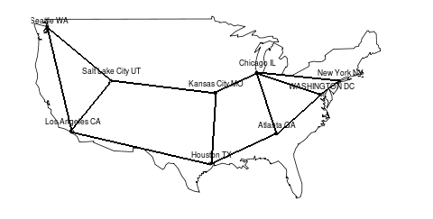
Figure 1: The Internet2 backbone network consists of $9$ nodes and $26$ one–directional links. All links have capacity of 10 Gbs/s, with the exception of the links: Chicago–Kansas, Kansas–Salt Lake City, New York–Washington, and Washington–Atlanta, all of which have doubled capacity of 20 Gbs/s in each direction.

NetFlow data: We obtained from [17], sampled measurements of all packets traversing the Internet2 (I2) backbone network (see Fig. 1). These data were used to reconstruct sampled versions of all flows $X_{j}(t),\ 1\leq j\leq{\cal J}=72$ in I2. Packet and bytes traces over the $100$ millisecond time scale were then obtained. The routing matrix $A$ for the I2 network was deduced from these NetFlow data sets as well and it was found to be constant in time.

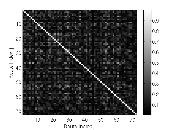
Figure 2: Correlation matrix (absolute values) of the flow–level traffic computed from a typical hour–long traces (in bytes per 10 sec). The traces are deduced from NetFlow measurements on the Internet2 backbone on Feb 19, 2009. Brighter shades indicate numbers close to $1$.

Computationally intensive processing is required to obtain the flow level data in practice. Therefore, these data cannot be used directly for fast on–line prediction of traffic. Nevertheless, we utilize this information to validate the main assumptions in our models. Fig. 2 indicates for example that the $X_{j}(t)$’s are nearly uncorrelated in $j$, which supports the simplifying independence assumption. On the other hand, the wavelet spectrum of a typical flow indicates that $X_{j}(t)$ is well–modeled by a fractional Gaussian noise time series for a wide range of time scales (see Fig. 3.) Further, barring a few anomalies in the NetFlow data, the Hurst exponents along most routes were found to be approximately equal (within statistical significance). These observations (along with NS2 simulation experiments, not discussed here due to lack space) support the overall validity global functional fBm model for the cumulative traffic fluctuations.

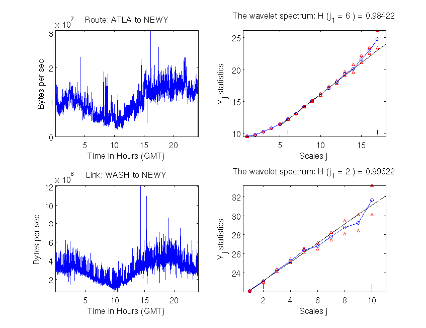
Figure 3: Top–left & right: a flow–level traffic trace (bytes per 100 msec) from Atlanta to New York for March 17, 2009 and its wavelet spectrum, which yields a Hurst parameter $\widehat{H}\approx 0.98$. Bottom–left & right: a link–level trace (bytes per 10 sec) for the Washington to New York link for March 17, 2009 and its wavelet spectrum with $\widehat{H}\approx 0.99$. Observe the similarity between the diurnal patterns and the Hurst exponents for the flow– and link–level data. The linearity of the wavelet spectra confirms the fractional Gaussian noise model.

Traffic traces: As indicated above, the NetFlow measurements cannot be used directly to readily predict the link loads in real time. We acquired from [17] time–synchronized traffic traces of packets and bytes on the $10$–second time scale, for all links in the Internet2 backbone network. As expected, since RTT $<<10$ sec, the routing equation (1) can be safely assumed to hold for the time scales of interest. By using coarse–scale information obtained from the corresponding NetFlow data, we approximated the mean $\mu_{X}$ and variance structure of the $X_{j}(t)$’s. Thus, by using $\mu_{X}$ and $\Sigma_{X}:={\rm diag}(\sigma_{X_{j}}^{2},\ 1\leq j\leq{\cal J}),$ we obtained from (15) the standard kriging estimator for a number of scenarios with observed and unobserved links.

Figs 4 and 5 demonstrate the success of our global modeling strategy in the context of network kriging. By monitoring just a few links, with the help of the standard kriging estimator described above, one can track relatively well the traffic load on other links. Table 1 shows further that a given link can be relatively well predicted from measurements of as few as two other links. The results also show that the choice of which set of link to monitor is an important design problem.

Number of links	Link labels	Relative m.s.e.
2	3,7	0.07
2	7,9	0.12
2	9,12	0.08
2	12,17	0.41
2	17,21	3.06
2	3,21	0.05
3	3,7,9	0.12
4	3,7,9,12	0.08
5	3,7,9,12,17	0.07
6	3,7,9,12,17,21	0.06
8	3,5,7,9,11,12,17,21	0.06
10	3,5,7,9,11,12,17,21,23,25	0.06

Table 1: Empirical relative mean squared error for the standard kriging estimator: ${\rm(r.m.s.e.)}\ =(\sum_{t=1}^{T}(\widehat{Y}_{u}(t)-Y_{u}(t))^{2})/(\sum_{t=1}^{T}Y_{u}(t)^{2})$. The Internet2 backbone link 13 (Kansas City to Chicago) was predicted from various sets of other backbone links. The data spans the entire day of February 19, 2009. The link ID’s are described in Table 2.

ID	Source–Destination	Cap.	ID	Source–Destination	Cap.
1	Los Angeles–Seattle	10 Gb/s	2	Seattle–Los Angeles	10 Gb/s
3	Seattle–Salt Lake City	10 Gb/s	4	Salt Lake City–Seatle	10 Gb/s
5	Los Angeles–Salt Lake City	10 Gb/s	6	Salt Lake City–Los Angeles	10 Gb/s
7	Los Angeles–Houston	10 Gb/s	8	Houston–Los Angeles	10 Gb/s
9	Salt Lake City–Kansas City	10 Gb/s	10	Kansas City–Salt Lake City	10 Gb/s
11	Kansas City–Houston	10 Gb/s	12	Houston–Kansas City	10 Gb/s
13	Kansas City–Chicago	20 Gb/s	14	Chicago–Kansas City	20 Gb/s
15	Houston–Atlanta	10 Gb/s	16	Atlanta–Houston	10 Gb/s
17	Chicago–Atlanta	10 Gb/s	18	Atlanta–Chicago	10 Gb/s
19	Chicago–New York	10 Gb/s	20	New York–Chicago	10 Gb/s
21	Chicago–Washington	10 Gb/s	22	Washington–Chicago	10 Gb/s
23	Atlanta–Washington	10 Gb/s	24	Washington–Atlanta	10 Gb/s
25	Washington–New York	20 Gb/s	26	New York–Washington	20 Gb/s

Table 2: A description of the 26 links that form the Internet2 backbone. Also provided are the id numbers used in this paper for notational simplicity.

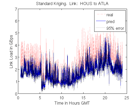
Figure 4: Prediction for the Internet2 backbone link Houston to Atlanta HOUS->ATLA based on the links: SEAT->SALT, SEAT->LOSA, LOSA->HOUS, ATLA->WASH, CHIC->NEWY. The traces reflect an entire day of activity (February 19, 2009). Observe the diurnal patterns and the utilization (see the caption of Fig. 1). The dotted lines indicate $95\%$ prediction bounds.

Figure 5: A zoomed–in portion of Fig. 4. Observe that the standard kriging estimator closely tracks the true traffic trace and note that the prediction bounds are adequate.

There are, however, objective limitations to the degree to which one can predict unobserved links from another set of links. The example in Fig. 6 was chosen to illustrate these limitations. Observe that even though the coarse–scale traffic mean is tracked somewhat, the standard kriging estimator fails to track the finer scale behavior and the prediction intervals are rather wide.

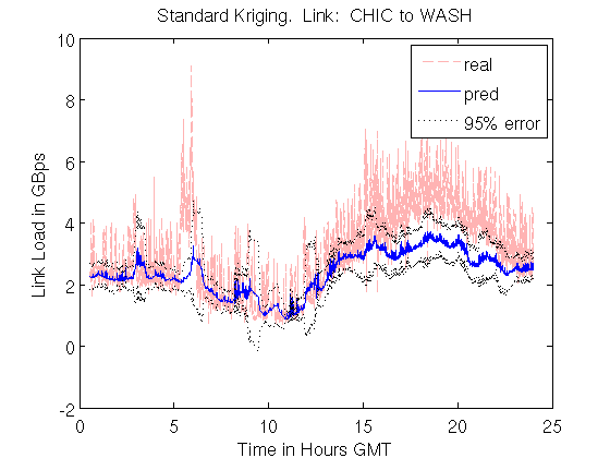
Figure 6: Prediction for the Internet2 backbone link Chicago to Washington based on the same set of observed links as in Fig. 4.

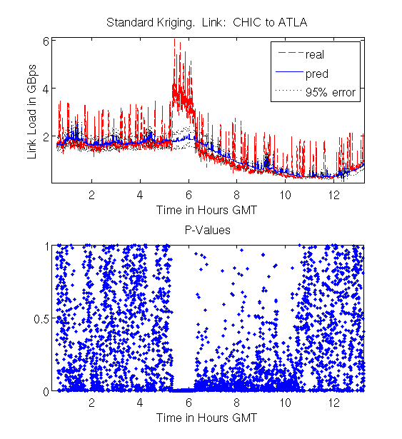
Figure 7: Top panel: standard kriging for CHIC->ATLA via the same set of observed links as in Fig. 4. Bottom panel: P–values corresponding to the top panel.

Fig. 7 shows that network kriging may be used in anomaly detection as a diagnostic device. Namely, one can predict an observed link from a set of other observed links and thus obtain a two–sided p–value based on the prediction distribution. Low p–values would indicate the presence of an anomaly. This is well demonstrated in Fig. 7 by drop in p–values between 5am and 6am GMT. The sudden peak load on the Chicago–Atlanta link is not tracked well by the monitored links and the underlying NetFlow data used to recover the overall mean and variance structure of the flow–level traffic. Thus, the network kriging methodology, based on our probabilistic model, provides an novel global view on the statistical significance of traffic patterns in the network.

6 Discussion

In this paper, we developed a probabilistic framework for network–wide modeling of traffic, based on multiple sources and large time–scale limit approximations. It is shown that depending on the scaling, a fast and slow regime occur in the limit. As an extension, one can also consider simultaneous limits as the number of sources $M=M(T)$ and as the time scale $T$ tend to infinity, as well as other complex asymptotic scenarios.

The proposed model proves mathematically tractable, involving few statistical parameters and therefore perfectly suitable for addressing a number of important questions for network–wide traffic behavior. As shown, the model can successfully predict traffic loads on unobserved links (network kriging), employing only a limited set of link measurements, provided that some coarse–scale information about the traffic means is available (e.g. through NetFlow data).

The developed network kriging methodology has further applications to anomaly detection and diagnostics, as shown in the example of Fig. 7. Since the model captures the joint distribution of all links in the network, the multiple testing problem associated with anomaly detection for a large number of links can be successfully handled, as well. Further, as illustrated in Fig. 6 and Table 1, in the presence of limited resources, it is important to select an “optimal set” of links for network monitoring; this model can be used to address this problem in the context of network kriging.

Finally, estimation of the joint distribution of means and covariances of traffic flows, across time and over the network, constitutes a challenging, but also important problem for network engineering. Our ongoing work is addressing this problem through flexible, parsimonious latent variable models that can be estimated in real time and without the need for the availability of NetFlow data [39].

7 Appendix

Proposition 8

The functional $(f,g)\mapsto\phi_{2H}(f,g)$ in (10) is positive semi–definite if and only if $0<H\leq 1$.

Proof: Since $(t,s)\mapsto\phi_{2H}(tf_{0},sf_{0}),\ t,s\in{\mathbb{R}}$ has the form of the auto–covariance of fBm, then it follows that necessarily $H\in(0,1]$ (see e.g. [30]). It remains to show that $\phi_{\alpha}$ is positive definite for all $\alpha:=2H\in(0,2]$.

Let $M_{\alpha},\ \alpha\in(0,2]$ be an S$\alpha$S random measure with control measure $\mu$ and define

$$\Lambda(f):=\int_{E}fdM_{\alpha},\ \ \forall f\in L^{\alpha}(\mu),$$

to be the S$\alpha$S integral of the deterministic function $f$ (see e.g. Ch. 3 in [30]). Notice that for all $x_{j}\in{\mathbb{C}},$ and $f_{j}\in L^{\alpha}(\mu)$, with $1\leq j\leq n$, we have

$${\mathbb{E}}{\Big{|}}\sum_{j=1}^{n}x_{j}e^{i\Lambda(f_{j})}{\Big{|}}^{2} = \sum_{j,k=1}^{n}x_{j}\overline{x}_{k}{\mathbb{E}}e^{i\Lambda(f_{j}-f_{k})}$$

$$= \sum_{j,k=1}^{n}x_{j}\overline{x}_{k}e^{-\|f_{j}-f_{k}\|_{\alpha}^{\alpha}}.$$

Since the l.h.s.  of the last expression is always non–negative, so is the r.h.s. This shows that the function $r_{\alpha}(f,g):=e^{-\|f-g\|_{\alpha}^{\alpha}},$ $f,g\in L^{\alpha}(\mu)$ is positive definite.

Now, the proof proceeds as the proof of the positive definiteness of the auto–covariance function of the fractional Brownian motion (see, e.g. p. 106 in [30]). Indeed, for all $x_{j}\in{\mathbb{C}},$ and $f_{j}\in L^{\alpha},\ 0\leq j\leq n$, and for all $\epsilon>0$, we have

$$0 \leq \sum_{j,k=0}^{n}x_{j}\overline{x}_{k}e^{-\epsilon\|f_{j}-f_{k}\|_{\alpha}^{\alpha}}$$

$$= \sum_{j,k=1}^{n}x_{j}\overline{x}_{k}e^{-\epsilon\|f_{j}-f_{k}\|_{\alpha}^{\alpha}}+\sum_{j=1}^{n}x_{0}\overline{x}_{k}e^{-\epsilon\|f_{0}-f_{k}\|_{\alpha}^{\alpha}}$$

$$\quad\quad+\sum_{j=1}^{n}x_{j}\overline{x}_{0}e^{-\epsilon\|f_{j}-f_{0}\|_{\alpha}^{\alpha}}+x_{0}\overline{x}_{0}$$

$$=: S_{1}+S_{2}+S_{3}+|x_{0}|^{2}$$

Since $x_{0}$ and $f_{0}$ are at our disposal, let $f_{0}:=0$ and $x_{0}:=-\sum_{j=1}^{n}x_{j}e^{-\epsilon\|f_{j}\|_{\alpha}^{\alpha}}$. Observe that with this choice of $x_{0}$ and $f_{0}$, we get

$$S_{2}=S_{3}=-|x_{0}|^{2}=-\sum_{j,k=1}^{n}x_{j}\overline{x}_{k}e^{-\epsilon\|f_{j}\|_{\alpha}^{\alpha}-\epsilon\|f_{k}\|_{\alpha}^{\alpha}},$$

and therefore, $S_{1}+S_{2}+S_{3}+|x_{0}|^{2}$ equals:

$$\sum_{j,k=1}^{n}x_{j}\overline{x}_{k}{\Big{(}}e^{-\epsilon\|f_{j}-f_{k}\|_{\alpha}^{\alpha}}-e^{-\epsilon\|f_{j}\|_{\alpha}^{\alpha}-\epsilon\|f_{k}\|_{\alpha}^{\alpha}}{\Big{)}}$$

$$= \epsilon\sum_{j,k=1}^{n}x_{j}\overline{x}_{k}{\Big{(}}\|f_{j}\|_{\alpha}^{\alpha}+\|f_{k}\|_{\alpha}^{\alpha}-\|f_{j}-f_{k}\|_{\alpha}^{\alpha}{\Big{)}}+o(\epsilon),$$

as $\epsilon\downarrow 0$, where the last relation we used the fact that $e^{-\epsilon a}-e^{-\epsilon b}=\epsilon(b-a)+o(\epsilon)$, as $\epsilon\downarrow 0$. If for some $x_{j}$’s and $f_{j}$’s we have $\sum_{j,k=1}^{n}x_{j}\overline{x}_{k}(\|f_{j}\|_{\alpha}^{\alpha}+\|f_{k}\|_{\alpha}^{\alpha}-\|f_{j}-f_{k}\|_{\alpha}^{\alpha})<0$, then, for all sufficiently small $\epsilon>0$, the l.h.s.  of (7) becomes negative, which in view of (7), is impossible. This shows that $\phi_{\alpha}$ is positive (semi–)definite.

Proof:[Proof of Prosition 1] To check the equality in distribution of two zero mean Gaussian processes, it is enough to show the equality of their auto–covariance functions. Let $1\leq\ell_{1},\ell_{2}\leq L$ and $t_{1},t_{2}\geq 0$. Then, by using the independence of the $B_{H}^{(j)}(t)$’s, we have:

$${\mathbb{E}}(A\vec{B}_{H}(t_{1}))_{\ell_{1}}(A\vec{B}_{H}(t_{2}))_{\ell_{2}}$$

$$\ \ \ \ \ =\sum_{1\leq u\leq{\cal J}}r(u)^{2}1_{A_{\ell_{1}}\cap A_{\ell_{2}}}(u)r_{2H}(t_{1},t_{2}),$$ (23)

where $r_{2H}(t_{1},t_{2})=(\sigma^{2}/2)(|t_{1}|^{2H}+|t_{2}|^{2H}-|t_{1}-t_{2}|^{2H})$. On the other hand, as in (3.2), we obtain

$${\mathbb{E}}B(t_{1}f_{\ell_{1}})B(t_{2}f_{\ell_{2}})=\frac{\sigma^{2}}{2}\sum_{1\leq u\leq{\cal J}}r(u)^{2}{\Big{(}}|t_{1}|^{2H}1_{A_{\ell_{1}}}(u)$$

$$\ \ \ \ \ +|t_{2}|^{2H}1_{A_{\ell_{2}}}(u)-|t_{1}1_{A_{\ell_{1}}}(u)-t_{2}1_{A_{\ell_{2}}}(u)|^{2H}{\Big{)}},$$

which after cancellations, equals the r.h.s. of (7).

Proof:[Proof of Proposition 2] (i): The auto–covariance function of the process $\{B(cf)\}_{f}$ is

$$\phi_{2H}(cf,cg)=\frac{\sigma^{2}}{2}{\Big{(}}\|cf\|^{2H}+\|cg\|^{2H}-\|cf-cg\|^{2H}{\Big{)}},$$

which equals ${\mathbb{E}}(c^{H}B(f))(c^{H}B(g))$, where $\|\cdot\|$ stands for $\|\cdot\|_{2H}$. This implies (11). The proof of (ii) is similar.

For simplicity, let now $\sigma=1$. Then

$${\mathbb{E}}(B(f+h)-B(h))(B(g+h)-B(h))$$

$$\ \ =\frac{1}{2}{\Big{(}}\|f+h\|^{2H}+\|g+h\|^{2H}-\|f-g\|^{2H}{\Big{)}}$$

$$\ \ \ \ -\frac{1}{2}{\Big{(}}\|h\|^{2H}+\|g+h\|^{2H}-\|g\|^{2H}{\Big{)}}$$

$$\ \ \ \ -\frac{1}{2}{\Big{(}}\|f+h\|^{2H}+\|h\|^{2H}-\|f\|^{2H}{\Big{)}}$$

$$\ \ \ \ \ +\|h\|^{2H}=\frac{1}{2}{\Big{(}}\|f\|^{2H}+\|g\|^{2H}-\|f-g\|^{2H}{\Big{)}},$$

which equals ${\mathbb{E}}B(f)B(f)$, and thus implies the equality of the finite–dimensional distributions in (12).

(iii) Since $fg=0$ $\mu-$a.e.

$$\|f-g\|^{2H} = \int_{E\cap\{f\not=0\}}|f|^{2H}d\mu+\int_{E\cap\{g\not=0\}}|g|^{2H}d\mu$$

$$\ \ \ =\|f\|^{2H}+\|g\|^{2H},$$

where for simplicity, $\sigma=1$. This implies the independence of $B(f)$ and $B(g)$, since ${\mathbb{E}}B(f)B(g)=\phi_{2H}(f,g)=0$ in view of (10).

Part (iv) follows trivially from (10). Now, to prove (v), it is enough to show ${\mathbb{E}}(B(f+g)-B(f)-B(g))^{2}=0$ if and only if $fg=0$ $\mu-$a.e. It can be shown that the last expectation equals:

$${\mathbb{E}}B(f+g)^{2}+{\mathbb{E}}B(f)^{2}+{\mathbb{E}}B(g)^{2}-2{\mathbb{E}}B(f+g)B(f)$$

$$\quad\quad\quad-2{\mathbb{E}}B(f+g)B(g)+2{\mathbb{E}}B(f)B(g)$$

$$\ \ \ =\|f+g\|^{2H}+\|f\|^{2H}+\|g\|^{2H}$$

$$\ \ \ \ -(\|f+g\|^{2H}+\|f\|^{2H}-\|g\|^{2H})$$

$$\ \ \ \ -(\|f+g\|^{2H}+\|g\|^{2H}-\|f\|^{2H})$$

$$\ \ \ +\|f\|^{2H}+\|g\|^{2H}-\|f-g\|^{2H}$$

$$\ \ \ =2\|f\|^{2H}+2\|g\|^{2H}-\|f-g\|^{2H}-\|f+g\|^{2H}.$$

Since $0<2H<2$, the last expression vanishes if and only if $fg=0$ $\mu-$a.e. (see Eq. (2.7.9) in Lemma 2.7.14 of [30]).

Proof:[Proof of Proposition 4] Let as in [30], $\|\xi\|_{\alpha}$ denote the scale coefficient of the $\alpha$ stable random variable $\xi$. To prove (i), it suffices to show that for all $f_{j}\in L^{1}(\mu)$, and $\theta_{j}\in{\mathbb{R}},\ 1\leq j\leq n$, we have that

$$\|\sum_{1\leq j\leq n}\theta_{j}\Lambda(cf_{j})\|_{\alpha}^{\alpha}=\|c^{1/\alpha}\sum_{1\leq j\leq n}\theta_{j}\Lambda(f_{j})\|_{\alpha}^{\alpha}.$$

The l.h.s. of this expression equals:

$$\int_{{\mathbb{R}}\times E}{\Big{|}}\sum_{1\leq j\leq n}\theta_{j}(1_{(-\infty,cf_{j}(u))}(x)-1_{(-\infty,0)}(x)){\Big{|}}^{\alpha}dx\mu(du).$$

By setting $z:=x/c$, we obtain that the last integral equals:

$$c\int_{{\mathbb{R}}\times E}{\Big{|}}\sum_{1\leq j\leq n}\theta_{j}(1_{(-\infty,f_{j}(u))}(z)-1_{(-\infty,0)}(z)){\Big{|}}^{\alpha}dz\mu(du),$$

which is

$$\|c^{1/\alpha}\sum_{1\leq j\leq n}\theta_{j}\Lambda(f_{j})\|_{\alpha}^{\alpha}.$$

This completes the proof of (i).

Part (ii) can be established similarly by using the Fubini’s theorem and the change of variables $z:=x-h(u)$ in the integral

$$\int_{{\mathbb{R}}\times E}{\Big{|}}\sum_{1\leq j\leq n}\theta_{j}(1_{(-\infty,f(u)+h(u))}(x)-1_{(-\infty,h(u))}(x)){\Big{|}}^{\alpha}dx\mu(du),$$

which equals $\|\sum_{1\leq j\leq n}\theta_{j}(\Lambda(f+h)-\Lambda(h))\|_{\alpha}^{\alpha}$.

(iii): In view of Theorem 3.5.3 in [30], $\Lambda(f)$ and $\Lambda(g)$ are independent if and only if

$$(1_{(-\infty,f(u))}(x)-1_{(-\infty,0)}(x))(1_{(-\infty,g(u))}(x)-1_{(-\infty,0)}(x))=0,$$

for $dx\times\mu(du)$ almost all $(x,u)$. By considering cases for the signs of $f(u)$ and $g(u)$, it follows that the latter equality holds (for $dx\times\mu(du)$ almost all $(x,u)$) if and only if $f(u)g(u)\leq 0$ $\mu(du)$–a.e.

(iv): Let $f_{0}:=0$ and observe that

$$\Lambda(f_{k})-\Lambda(f_{k-1})=\int_{{\mathbb{R}}\times E}1_{A_{k}}(x,u)M_{\alpha}(dx,du),$$

where $A_{k}=\{(x,u):f_{k-1}(u)\leq x<f_{k}(u)\}$, for $1\leq k\leq n$. Again, by Theorem 3.5.3 in [30], we have that the above increments are independent, if and only if, the sets $A_{k},\ 1\leq k\leq n$ are mutually disjoint (mod $dx\times d\mu$), which is clearly the case here.

The proof of (v) is similar to that of (iv).

(vi): Follows (ii) and part (iv) applied to the independent processes $\Lambda(tf_{+})$ and $\Lambda(tf_{-})$, where $f_{\pm}=\max\{\pm f,0\}$ since $\Lambda(tf)=\Lambda(tf_{+})-\Lambda(tf_{-}).$

Proof:[Proof of Proposition 5] To prove that ${\mathbb{E}}B(f)B(g)=\phi_{2H}(f,g)$, it suffices to show that

$${\rm Var}(B(f)-B(g))={\mathbb{E}}(B(f)-B(g))^{2}=\sigma^{2}\|f-g\|_{2H}^{2H}.$$

This is indeed the case: By using changes of variables and Fubini’s theorem, we have that

$${\mathbb{E}}(B(f)-B(g))^{2}$$

$$\ \ \ =\int_{{\mathbb{R}}\times E}{\Big{(}}(f(u)-x)_{+}^{H-1/2}-(g(u)-x)_{+}^{H-1/2}{\Big{)}}^{2}dx\mu(du),$$

equals

$$\int_{{\mathbb{R}}\times E}|f(u)-g(u)|^{2H-1}{\Big{(}}(1-x/c(u))_{+}^{H-1/2}$$

$$\ \ \ \ -(-x/c(u))_{+}^{H-1/2}{\Big{)}}^{2}dx\mu(du)$$

$$\ =\sigma^{2}\int_{E}|f(u)-g(u)|^{2H}\mu(du)=\sigma^{2}\|f-g\|_{2H}^{2H},$$

where $c(u)=f(u)-g(u)$ and $\sigma^{2}=\int_{{\mathbb{R}}}((1-x)_{+}^{H-1/2}-(-x)_{+}^{H-1/2})^{2}dx$.

Proof:[Proof of Proposition 6] Let $\mu_{Y}={\mathbb{E}}Y(t_{0})=(\mu_{u}^{t},\ \mu_{o}^{t})^{t}$ and

$$\Sigma_{Y}={\mathbb{E}}(Y(t_{0})-\mu_{Y})(Y(t_{0})-\mu_{Y})^{t}=\left(\begin{array}[]{ll}\Sigma_{uu}&\Sigma_{uo}\\ \Sigma_{ou}&\Sigma_{oo}\end{array}\right),$$

where $\Sigma_{ij}=A_{i}\Sigma_{X}A_{j}^{t},\ i,j\in\{o,u\}$. The conditional distribution of $Y_{u}(t_{0})|Y_{o}(t_{0})$ is Gaussian and:

$$Y_{u}(t_{0})|Y_{o}(t_{0})\sim{\cal N}(\mu_{u}+\Sigma_{uo}\Sigma^{-1}_{oo}(Y_{o}-\mu_{o}),\Sigma_{uu}-\Sigma_{uo}\Sigma^{-1}_{oo}\Sigma_{ou})$$ (24)

(see eg Theorem 1.6.6 in [4]). Thus, an unbiased predictor of $Y_{u}(t_{0})$, given $Y_{o}(t_{0})$ is:

$$\widehat{Y}_{u}(t_{0}):={\mathbb{E}}(Y_{u}(t)|Y_{o}(t))=\mu_{u}+\Sigma_{uo}\Sigma^{-1}_{oo}(Y_{o}-\mu_{o}).$$ (25)

This implies (15) and (16) with ${\cal D}$ replaced by $Y_{o}(t_{0})$. Proposition 9 below implies, however, that $\widehat{Y}_{u}(t_{0})-Y_{u}(t_{0})$ and $Y_{o}(t)$ are uncorrelated, for all $t_{0}-m\leq t\leq t_{0}$. This completes the proof of (i).

To prove (ii), let $\theta$ be a constant vector of the same dimension as $Y_{u}(t_{0})$. Consider the random variable $\xi:=\theta^{t}Y_{u}(t_{0})$. It is well–known that ${\mathbb{E}}(\xi|Y_{o}(t_{0}))$ is the best unbiased m.s.e. predictor of $\xi$ via $Y_{o}(t_{0})$. Thus

$$\theta^{t}{\rm m.s.e.}(\widehat{Y}_{u}(t_{0})|Y_{o}(t_{0}))\theta\leq\theta^{t}{\rm m.s.e.}(Y_{u}^{*}(t_{0})|Y_{o}(t_{0}))\theta,$$

which implies (ii) and completes the proof.

The following result shows that if the space–time covariance structure of a random field factors, then the instantaneous standard kriging estimate is an optimal linear predictor even in the presence of additional data from the past.

Proposition 9

Let $\{\xi(t,x)\}_{(t,x)\in T\times S}$ be a finite variance space–time random field. Suppose that ${\mathbb{E}}\xi(t,x)=0$, for all $(t,x)\in T\times S$ and that

$${\rm Cov}(\xi(t,x),\xi(s,y))=\gamma(t,s)R(x,y),$$

for all $t,s\in T$ and $x,y\in S.$ Consider the data set ${\cal D}=\{\xi(t_{i},x_{j}),\ 0\leq i\leq m,\ 1\leq j\leq n\}$ of observations of the random field at times $t_{0},t_{1},\cdots,t_{m}$ and locations $x_{1},\cdots x_{n}$. Then, there exist coefficients $\beta_{j},1\leq j\leq n$, such that

$$\widehat{\xi}(t_{0},x_{0}):=\sum_{j=1}^{n}\beta_{j}\xi(t_{0},x_{j})$$ (26)

is the best linear in ${\cal D}$, unbiased predictor of $\xi(t_{0},x_{0})$. In particular, we have

$$\vec{\beta}=\Sigma_{t_{0}}^{-}\vec{c},\ \ \mbox{ where }\ \ \Sigma_{t_{0}}=({\rm Cov}(\xi(t_{0},x_{i}),\xi(t_{0},x_{j})))_{n\times n}$$ (27)

and $\vec{c}=({\rm Cov}(\xi(t_{0},x_{0}),\xi(t_{0},x_{i})))_{i=1}^{n}$. Here $\Sigma_{t_{0}}^{-}$ denotes the Moore–Penrose generalized inverse of the covariance matrix $\Sigma_{t_{0}}$.

Proof: Consider the Hilbert space ${\cal L}^{2}$ of finite variance random variables with zero means and the usual inner product $\langle\xi,\eta\rangle:={\mathbb{E}}\xi\eta$. Consider the sub–space $W={\rm span}({\cal D})\leq{\cal L}^{2}$ and observe that the best linear in ${\cal D}$ unbiased predictor for $\xi(t_{0},x_{0})$ is the (unique) orthogonal projection of $\xi(t_{0},x_{0})$ onto $W$.

Let $\widehat{\xi}(t_{0},x_{0})$ be the orthogonal projection of $\xi(t_{0},x_{0})$ onto the smaller subspace ${\rm span}\{\xi(t_{0},x_{j}),\ 1\leq j\leq n\}$. We then have that, for all $k=1,\cdots,n$

$$0 = {\rm Cov}{\Big{(}}(\xi(t_{0},x_{0})-\sum_{j=1}^{n}\beta_{j}\xi(t_{0},x_{j})),\ \xi(t_{0},x_{k}){\Big{)}}$$

$$= \gamma(t_{0},t_{0})R(x_{0},x_{k})-\sum_{j=1}^{n}\beta_{j}\gamma(t_{0},t_{0})R(x_{j},x_{k}).$$

This, since $\gamma(t_{0},t_{0})\not=0$, shows that

$$R(x_{0},x_{k})-\sum_{j=1}^{n}\beta_{j}R(x_{j},x_{k})=0,\ \ \mbox{ for all }1\leq k\leq n.$$ (28)

We will show next that $\xi(t_{0},x_{0})-\sum_{j=1}^{n}\beta_{j}\xi(t_{0},x_{j})$ is orthogonal to $\xi(t_{i},x_{k})$ for all $i=1,\cdots,m$ and $k=1,\cdots,n$. Indeed,

$${\rm Cov}{\Big{(}}\xi(t_{0},x_{0})-\sum_{j=1}^{n}\beta_{j}\xi(t_{0},x_{j}),\xi(t_{i},x_{k}){\Big{)}}$$

$$\ \ \ =\gamma(t_{0},t_{i})R(x_{0},x_{k})-\sum_{j=1}^{n}\beta_{j}\gamma(t_{0},t_{i})R(x_{j},x_{k})$$

$$\ \ \ =\gamma(t_{0},t_{i}){\Big{(}}R(x_{0},x_{k})-\sum_{j=1}^{n}\beta_{j}R(x_{j},x_{k}){\Big{)}}=0,$$

where the last term vanishes because of (28). This implies that $\widehat{\xi}(t_{0},x_{0})$ is in fact the orthogonal projection of $\xi(t_{0},x_{0})$ onto $W$ and hence, it is the b.l.u.p. in terms of the data in ${\cal D}$.

Relation (27) follows by solving (28). If $\Sigma_{t_{0}}$ is invertible, then the solution is certainly unique, otherwise the Moore–Penrose generalized inverse $\Sigma_{t_{0}}^{-}$ yields a particular natural solution.

Proof:(Proposition 7) Part (i) is standard in one dimension (see eg Corollary 5.1.1 in [4]). For completeness, we will prove the result in the case when $Y_{o}(t)\in{\mathbb{R}}^{d}$. Let $\Sigma_{oo}=A_{o}\Sigma_{X}A_{o}^{t}$ and observe that ${\mathbb{E}}(Y_{o}(t)-\mu_{o})(Y_{o}(s)-\mu_{o})^{t}=\gamma_{X}(|t-s|)\Sigma_{oo}$.

Consider now the zero mean Gaussian vectors: $\xi:=Y_{o}(t_{0}+h)-\mu_{o}$ and

$$\eta=(Y_{o}(t_{0})^{t}-\mu_{o}^{t},\ \cdots,\ Y_{o}(t_{0}-m)^{t}-\mu_{o}^{t})^{t}.$$

Note that $\xi\sim{\cal N}(0,\Sigma_{oo})$ and $\eta\sim{\cal N}(0,\Gamma_{m+1}\otimes\Sigma_{oo})$, where ’$\otimes$’ denotes the Kronecker product:

$$\Gamma_{m+1}\otimes\Sigma_{oo}={\Big{(}}\gamma_{X}(|i-j|)\Sigma_{oo}{\Big{)}}_{(m+1)d\times(m+1)d},$$

and where $\Sigma_{oo}$ is a $d\times d$ matrix. By assumption, we have that $\Sigma_{oo}$ is invertible, and as argued above, so is the Toeplitz matrix $\Gamma_{m+1}$, since $\gamma_{X}(k)\to 0,\ k\to\infty$ (Proposition 5.1.1 in [4]). This implies that $\Sigma_{\eta\eta}^{-1}:=(\Gamma_{m+1}\otimes\Sigma_{oo})^{-1}=\Gamma_{m+1}^{-1}\otimes\Sigma_{oo}^{-1}$ exists. Therefore, the conditional distribution $\xi|\eta$ is as follows:

$$\xi|\eta\sim{\cal N}{\Big{(}}\Sigma_{\xi\eta}\Sigma_{\eta\eta}^{-1}\eta,\ \Sigma_{\xi\xi}-\Sigma_{\xi\eta}\Sigma_{\eta\eta}^{-1}\Sigma_{\eta\xi}{\Big{)}},$$ (29)

where

$$\Sigma_{\xi\eta}={\mathbb{E}}\xi\eta^{t}=\vec{\gamma}_{m+1}(h)^{t}\otimes\Sigma_{oo},\ \ \ \Sigma_{\eta\eta}={\mathbb{E}}\eta\eta^{t}=\Gamma_{m+1}\otimes\Sigma_{oo},$$

and

$$\Sigma_{\eta\xi}=\vec{\gamma}_{m+1}(h)\otimes\Sigma_{oo}.$$

By recalling the definitions of $\xi$ and $\eta$, we obtain that

$${\mathbb{E}}(Y_{o}(t_{0}+h)|{\cal D})=\mu_{o}+{\mathbb{E}}(\xi|\eta)$$

$$\ \ \ \ =\mu_{o}+(\vec{\gamma}_{m+1}(h)^{t}\otimes\Sigma_{oo})(\Gamma_{m+1}^{-1}\otimes\Sigma_{oo}^{-1})\eta$$

$$\ \ \ \ =\mu_{o}+(\vec{\gamma}_{m+1}(h)^{t}\Gamma_{m+1}^{-1})\otimes{{\mathbb{I}}}_{d})\eta,$$

which equals (18), and where in the last relation we used the mixed–product property of the Kronecker product. By Relation (29), we also have

$${\rm m.s.e.}(\widehat{Y}_{o}(t_{0}+h)|{\cal D})=\Sigma_{\xi\xi}-\Sigma_{\xi\eta}\Sigma_{\eta\eta}^{-1}\Sigma_{\xi\eta}=\gamma_{X}(0)\Sigma_{oo}$$

$$\ \ -(\vec{\gamma}_{m+1}(h)^{t}\otimes\Sigma_{oo})(\Gamma_{m+1}^{-1}\otimes\Sigma_{oo}^{-1})(\vec{\gamma}_{m+1}(h)\otimes\Sigma_{oo})$$

$$=\gamma_{X}(0)\Sigma_{oo}$$

$$\ \ -(\vec{\gamma}_{m+1}(h)^{t}\Gamma_{m+1}^{-1}\gamma_{m+1}(h))\otimes\Sigma_{oo}\equiv\sigma^{2}(h)\Sigma_{oo},$$

by the mixed–product property of the Kronecker product and the fact that $\gamma_{m+1}(h)^{t}\Gamma_{m+1}^{-1}\gamma_{m+1}(h)$ is a scalar. We have thus shown (19).

We now focus on proving (ii). Consider $Y_{o}(t_{0}+h)$ and write

$$\widehat{Y}_{u}(t_{0}+h):=\mu_{u}+C(Y_{o}(t_{0}+h)-\mu_{o})+C(\widehat{Y}_{o}(t_{0}+h)-Y_{o}(t_{0}+h)).$$

As in Proposition 6, one can show that $Y_{u}(t_{0}+h)-CY_{o}(t_{0}+h)$ is independent from $Y_{o}(t)$, for all $t\leq t_{0}+h$. Therefore,

$${\rm m.s.e.}(\widehat{Y}_{u}(t_{0}+h)|{\cal D}) = {\rm m.s.e.}(\widehat{Y}_{u}(t_{0}+h)|Y_{o}(t_{0}+h))$$

$$\ \ \ +C{\rm m.s.e.}(\widehat{Y}_{o}(t_{0}+h)|{\cal D})C^{t},$$

where in the last relation ${\rm m.s.e.}(\widehat{Y}_{u}(t_{0}+h)|Y_{o}(t_{0}+h))$ stands for the m.s.e. of the standard Kriging estimator in Relation (16) and where ${\rm m.s.e.}(\widehat{Y}_{o}(t_{0}+h)|{\cal D})$ is as in (19). This completes the proof of (ii).

To prove (iii) observe that the estimator in (i) is the conditional expectation of $Y_{o}(t_{0}+h)$ given ${\cal D}$ and it is therefore the best m.s.e. predictor. If $Y(t)$ is non–Gaussian, this yields only the b.l.u.p. By Proposition 6, we have that

$${\mathbb{E}}{\Big{(}}Y_{u}(t_{0}+h)\,|\,\{Y_{o}(t),\ t\leq t_{0}+h\}{\Big{)}}=\mu_{u}+C(Y_{o}(t_{0}+h)-\mu_{o}),$$

on the other hand, by part (i), we have that

$${\mathbb{E}}{\Big{(}}\mu_{u}+C(Y_{o}(t_{0}+h)-\mu_{o})|{\cal D}{\Big{)}}=\mu_{u}+C(\widehat{Y}_{o}(t_{0}+h)-\mu_{o}).$$

The last two relations yield: ${\mathbb{E}}{\Big{(}}Y_{u}(t_{0}+h)|{\cal D}{\Big{)}}=\mu_{u}+C(\widehat{Y}_{o}(t_{0}+h)-\mu_{o}),$ which shows that $\widehat{Y}_{u}(t_{0}+h)$ is the best m.s.e. predictor. In the non–Gaussian case, this is merely the b.l.u.p.

References

• [1] P. Abry and D. Veitch. Wavelet analysis of long range dependent traffic. IEEE Transactions on Information Theory, 44(1):2–15, 1998.
• [2] N. Antunes, A. Pacheco, and R. Rocha. An integrated traffic model for multimedia wireless networks. Computer Networks, 38: 25–41, 2002.
• [3] J.-M. Bardet, G. Lang, G. Oppenheim, A. Philippe, S. Stoev, and M.S. Taqqu. Semi-parametric estimation of the long-range dependence parameter : A survey. In P. Doukhan, G. Oppenheim, and M. S. Taqqu, editors, Theory and Applications of Long-range Dependence, pages 579–623. Birkhäuser, 2003.
• [4] P. J. Brockwell and R. A. Davis. Time Series: Theory and Methods. Springer-Verlag, New York, 2nd edition, 1991.
• [5] D.B. Chua, E.D. Kolaczyk, and M. Crovella. Network kriging. Selected Areas in Communications, IEEE Journal on, 24(12):2263–2272, Dec. 2006.
• [6] N. Cressie. Statistics for Spatial Data: revised ed. John Wiley, New York, 1993.
• [7] M. E. Crovella and A. Bestavros. Self-similarity in World Wide Web traffic: evidence and possible causes. In Proceedings of the 1996 ACM SIGMETRICS. International Conference on Measurement and Modeling of Complex Systems, pages 160–169, May 1996.
• [8] M. E. Crovella, M. S. Taqqu, and A. Bestavros. Heavy-tailed probability distributions in the World Wide Web. In R. Adler, R. Feldman, and M. S. Taqqu, editors, A Practical Guide to Heavy Tails: Statistical Techniques and Applications, pages 3–25, Boston, 1998. Birkhäuser.
• [9] B. D’Auria and G. Samorodnitsky. Limit behavior of fluid queues and networks. Oper. Res., 53(6):933–945, 2005.
• [10] N.G. Duffield. Sampling for passive Internet measurement: a review. Statistical Science, 19:472-–498, 2004.
• [11] P. Embrechts and M. Maejima. Selfsimilar processes, Princeton Series in Applied Mathematics, Princeton University Press, 2002.
• [12] A. Erramilli, P. Pruthi, and W. Willinger. Self-similarity in high-speed network traffic measurements: Fact or artifact? In Proceedings of the 12th Nordic Teletraffic Seminar NTS12, Espoo, Finland, pages 299–310, 1995.
• [13] Network traffic behaviour in switched Ethernet systems. Performance Evaluation, 58: 243–360.
• [14] R. Gaigalas and I. Kaj. Convergence of scaled renewal processes and a packet arrival model. Bernoulli, 9(4):671–703, 2003.
• [15] W.B. Gong, Y. Liu, V. Misra, and D. Towsley. Self-similarity and long range dependence on the internet: a second look at the evidence, origins and implications Computer Networks, 48: 377-399, 2005.
• [16] N. Hohn, D. Veitch, and P. Abry. Cluster processes, a natural language for network traffic IEEE Transactions on Signal Processing, 51(8): 2229–2244, 2003.
• [17] Internet2: http://www.internet2.edu/observatory/
• [18] A. Lakhina, K. Papagiannaki, M. Crovella, C. Diot, E.D. Kolaczyk, and N. Taft􏲩. Structural analysis of network trafic flows. Proceedings of Sigmetrics, 2004.
• [19] E. Lawrence, G. Michailidis, V.N. Nair and B. Xi. Network tomography: a review and recent developments. in Frontiers in Statistics, J. Fan and H. Koul (eds), 345–364, 2006.
• [20] On the self-similar nature of Ethernet traffic. Computer Communications Review, 23:183–193, 1993. Proceedings of the ACM/SIGCOMM’93, San Francisco, September 1993.
• [21] A. Lombardo, G. Morabito, and G. Schembra. A novel analytical framework compounding statistical traffic modeling and aggregate-Level service curve disciplines: network performance and efficiency implications. IEEE/ACM Trans. on Networking, 12: 443-456, 2004.
• [22] T. Mikosch, S. Resnick, H. Rootzén, and A. Stegeman. Is network traffic approximated by stable Lévy motion or fractional Brownian motion? The Annals of Applied Probability, 12(1):23–68, 2002.
• [23] T. Mikosch, and S. Resnick. Activity rates with very heavy tails. Stochastic Process. Appl., 116(2):131–155, 2006.
• [24] T. Mikosch, and G. Samorodnitsky. Scaling limits for cumulative input processes. Math. Oper. Res., 32(4):890–918, 2007.
• [25] K. Park, G. Kim, and M. E. Crovella. On the relationship between file sizes, transport protocols, and self-similar network traffic. In Proceedings of the Fourth International Conference on Networks Protocols (ICNP’96), October 1996.
• [26] K. Park and W. Willinger, editors. Self-Similar Network Traffic and Performance Evaluation. J. Wiley & Sons, Inc., New York, 2000.
• [27] Y. Paschalidis, and G. Smaragdakis. Spatio-temporal network anomaly detection by assessing deviations of empirical measures. IEEE/ACM Trans. on Networking, 17: 685–697, 2009.
• [28] V. Pipiras, M. S. Taqqu, and J. B. Levy. Slow, fast and arbitrary growth conditions for renewal-reward processes when both the renewals and the rewards are heavy-tailed. Bernoulli, 10(1):121–163, 2004.
• [29] D. Rolls, F. Hernandez-Campps, and G. Michailidis. Queueing analysis of network traffic: methodology and visualization tools. Computer Networks, 48:447–473, 2005.
• [30] G. Samorodnitsky and M. S. Taqqu. Stable Non-Gaussian Processes: Stochastic Models with Infinite Variance. Chapman and Hall, New York, London, 1994.
• [31] H. Singhal, and G. Michailidis. Identifiability of flow distributions from link measurements with applications to computer networks. Inverse Problems, 23: 1821–1850, 2007.
• [32] S. Stoev, V. Pipiras, and M. S. Taqqu. Estimation of the self-similarity parameter in linear fractional stable motion. Signal Processing, 82:1873–1901, 2002.
• [33] S. Stoev, M. Taqqu, C. Park, G. Michailidis, and J. S. Marron. LASS: a tool for the local analysis of self-similarity. Computational Statistics and Data Analysis, 50:2447–2471, 2006.
• [34] S. Stoev and M. S. Taqqu. Wavelet estimation for the Hurst parameter in stable processes. In Govindan Rangarajan and Mingzhou Ding, editors, Processes with Long-Range Correlations: Theory and Applications, pages 61–87, Berlin, 2003. Springer Verlag. Lecture Notes in Physics 621.
• [35] S. Stoev, M. S. Taqqu, C. Park, and J. S. Marron. On the wavelet spectrum diagnostic for Hurst parameter estimation in the analysis of Internet traffic. Computer Networks, 48:423–445, 2005.
• [36] S. Stoev and M. S. Taqqu. Asymptotic self-similarity and wavelet estimation for long-range dependent fractional autoregressive integrated moving average time series with stable innovations. J. Time Ser. Anal., 26(2):211–249, 2005.
• [37] M. S. Taqqu and V. Teverovsky. Semi-parametric graphical estimation techniques for long-memory data. In P. M. Robinson and M. Rosenblatt, editors, volume 115 of Lecture Notes in Statistics, pp 420–432, New York, 1996. Springer-Verlag.
• [38] M. S. Taqqu, W. Willinger, and R. Sherman. Proof of a fundamental result in self-similar traffic modeling. Computer Communications Review, 27(2):5–23, 1997.
• [39] J. Vaughan, S. Stoev, and G. Michailidis. Global modeling and prediction of computer network traffic. Working paper, 2009.
• [40] W. Willinger, M. S. Taqqu, R. Sherman, and D. V. Wilson. Self-similarity through high-variability: statistical analysis of Ethernet LAN traffic at the source level. IEEE/ACM Transactions in Networking, 5(1):71–86, 1997.
• [41] K. Xu, Z.L. Zhang, and S. Bhattacharyya. Profiling Internet backbone traffic: behavior models and applications. Proceedings of Sigcomm, 2005.
• [42] L. Yang, and G. Michailidis. Sample based estimation of network traffic flow characteristics. Proceedings of Infocom, 2007