TΘΔΘΔ\Theta\Delta

Real space estimator for the weak lensing convergence from the CMB

C.S. Carvalho111Corresponding author: carvalho.c@gmail.com and K. Moodley Astrophysics and Cosmology Research Unit, School of Mathematical Sciences, University of KwaZulu-Natal, 4000 Durban, South Africa
(March 3, 2024)
Abstract

We propose an estimator defined in real space for the reconstruction of the weak lensing potential due to the intervening large scale structure from high resolution maps of the cosmic microwave background. This estimator was motivated as an alternative to the quadratic estimator in harmonic space to surpass the difficulties of the analysis of maps containing galactic cuts and point source excisions. Using maps synthesised by pixel remapping, we implement the estimator for two experiments, namely one in the absence and one in the presence of detector noise, and compare the reconstruction of the convergence field with that obtained with the quadratic estimator defined in harmonic space. We find good agreement between the input and the reconstructed power spectra using the proposed real space estimator. We discuss interesting features of the real space estimator and future extensions of this work.

I Introduction

Observations of the cosmic microwave background (CMB) are a powerful probe of the physics of the early universe and a robust discriminant of cosmological models. Since the CMB photons propagate more or less freely after recombination, what we observe on large scales are mainly the perturbations on the last-scattering surface. The CMB contains also an imprint of the photon quadrupole which developed during the recombination epoch and generated linear polarisation through the mechanism of Thomson scattering.

However, the CMB should also contain signatures of processes that occurred between the last-scattering surface and the present. These processes will be manifest as non-linear signals which become important on small scales. The growing improvement in resolution and sensitivity of CMB experiments allows us to resolve ever so smaller scales and motivates the development of estimators and robust implementations for the extraction of the different signals. Among such processes is weak gravitational lensing, which consists of the deflection of CMB photons by the mass of matter clustered along the line of sight, while leaving the surface brightness unaffected. This effect distorts the temperature-temperature (TT) correlation power spectrum by a few arcminutes but coherently over degree scales seljak , which means that lensing becomes an important effect for 3000.3000\ell\geq 3000. Weak lensing also mixes and distorts the EE and BB polarisation power spectra zaldarriaga&seljak . Finally, weak lensing also correlates with other secondary effects, such as the integrated Sachs-Wolfe (ISW) effect and the Sunyaev-Zel’dovich (SZ) effect, thus inducing non-Gaussianities which are manifest in higher-order point correlation functions zaldarriaga ; cooray .

The relevance of the CMB lensing reconstruction for cosmology is threefold. First, by converting a fraction of the dominant E-mode polarisation due to density perturbations into a B-mode polarisation, CMB lensing introduces a contaminant in the measurement of the primordial B-mode polarisation and consequently of the inflation energy scale gravitational_waves . Second, CMB lensing is also a powerful cosmological probe of the matter distribution integrated from the last scattering surface at redshift z1000similar-to𝑧1000z\sim 1000 to the present time. Third, by changing the power spectra of the perturbations and inducing non-Gaussianities, CMB lensing affects cosmological parameter estimation. Delensing the CMB will thus allow one to recover the primordial B-mode, probe the full-sky large-scale structure distribution with a maximum efficiency at z3𝑧3z\approx 3 lewis&challinor , and obtain unbiased parameter constraints from CMB measurements lewis .

Effort has been devoted to developing an optimal reconstruction of the lensing potential in harmonic space, which implicitly assumes full-sky coverage without galactic cuts, bad pixels due to excision of point sources or nonuniform weighting for uneven sky coverage okamoto&hu . In this idealized context, it has been shown how to construct an optimal quadratic estimator for a reconstruction based on the temperature anisotropy alone hu (see hu&okamoto for an extension of the formalism to include the polarisation). The improvement gained from using a maximum likelihood, and thus more optimal, estimator for the reconstruction from the temperature is marginal hirata&seljak2002 (although this might not necessarily be the case for experiments sensitive to the B-mode polarisation hirata&seljak2003 ). This is because the distortion due to lensing is small compared to the intrinsic cosmic variance or to the experimental noise.

Our interest lies in considering a slightly less optimal estimator modified to have a finite range in real space. The estimator is based on a convolution of the square of the lensed temperature map with a local kernel, as has been suggested previously bucher . An estimator with kernel in real space acts locally, as opposed to the conventional estimator with kernel in harmonic space which acts over the entire celestial sphere even though it has finite support in harmonic space. The extent in real space will be the inverse of that in harmonic space, thus finite and determined by the scale of the root mean square of the lensing convergence, with the contribution from sources beyond the kernel being negligible. An estimator with these properties can easily be adapted to include cuts, excisions of pixels and nonuniform sky coverage for a local extraction of the lensing convergence. In particular, a nonuniform sky coverage can be accounted for by a corresponding weighting in the real space convolution.

The lensing distortion of the CMB anisotropy on the surface of last scattering can be described in three ways: by the lensing potential ψ,𝜓\psi, by the deflection vector 𝜶=ψ𝜶𝜓\boldsymbol{\alpha}=\nabla\psi or by the convergence tensor 𝜿=ψ/2.𝜿𝜓2\boldsymbol{\kappa}=-\nabla\nabla\psi/2. The descriptions of ψ𝜓\psi and 𝜶𝜶\boldsymbol{\alpha} suffer from an ambiguity upon translation, since a patch of the sky and its translation have the same likelihood on account of isotropy. In contrast, the description of the convergence, which is a gradient of the deflection vector field, is locally well defined. Here we implement the real space estimator to reconstruct the convergence and compare the reconstruction to that obtained with the harmonic space estimator.

The convergence tensor can be decomposed as a sum of an isotropic (diagonal) tensor and an anisotropic (traceless) tensor as follows

𝜿=(κ0+κ+κ×κ×κ0κ+).𝜿subscript𝜅0subscript𝜅subscript𝜅subscript𝜅subscript𝜅0subscript𝜅\displaystyle\boldsymbol{\kappa}=\left(\begin{array}[]{cc}\kappa_{0}+\kappa_{+}&\kappa_{\times}\\ \kappa_{\times}&\kappa_{0}-\kappa_{+}\end{array}\right). (3)

For a small patch of sky, we can use the flat-sky approximation and define a Cartesian coordinate system with basis vectors {𝒆x(r),𝒆y(r)}subscript𝒆𝑥𝑟subscript𝒆𝑦𝑟\{\boldsymbol{e}_{x}(r),\boldsymbol{e}_{y}(r)\} and metric g=diag(1,1).𝑔diag11g={\rm diag}(1,1). In particular, the convergence κ0=(x2+y2)ψ/2subscript𝜅0superscriptsubscript𝑥2superscriptsubscript𝑦2𝜓2\kappa_{0}=-(\partial_{x}^{2}+\partial_{y}^{2})\psi/2 magnifies a feature on the last-scattering surface, the shear κ+=(x2y2)ψ/2subscript𝜅superscriptsubscript𝑥2superscriptsubscript𝑦2𝜓2\kappa_{+}=-(\partial_{x}^{2}-\partial_{y}^{2})\psi/2 stretches it along the x𝑥x–axis while compressing it along the y𝑦y–axis, and analogously the shear κ×=xyψsubscript𝜅subscript𝑥subscript𝑦𝜓\kappa_{\times}=-\partial_{x}\partial_{y}\psi stretches it along the y=x𝑦𝑥y=x axis and compresses it along the y=x𝑦𝑥y=-x axis. Here we focus on the dilation effect captured by the isotropic component κ0,subscript𝜅0\kappa_{0}, and will treat the shear components in a forthcoming study.

The convergence can be further decomposed into two contributions, namely the convergence of the unlensed temperature anisotropies, to a high degree isotropic, and the convergence of the lensing field, by nature random. In order to remove the zero mode of the unlensed CMB, we average the convergence on each local patch over the sky region surveyed and subtract this average value from the estimated convergence map. Higher multipoles of the unlensed CMB will still be present in the estimated convergence map, which give rise to a noise bias. This bias can be removed by cross-correlating the reconstructed map with maps of the large scale structure derived from independent methods, e.g. a galaxy redshift survey. It can also be removed when estimating the convergence power spectrum by combining, in harmonic space, different triangle configurations with a common side. The formulation of an estimator for the lensing convergence given the lensed image still requires some prior knowledge of the statistics of the underlying temperature field, in particular the power spectrum of the unlensed sky which is assumed to be Gaussian.

This is the first of a series of studies where we explore the properties of the proposed estimator and test its implementation. The manuscript is organized as follows. In Section II we describe the weak lensing CMB of photons in the Born approximation. In Section III we derive the proposed estimator defined in real space, whose kernel in harmonic space is described in Appendix A. In Section IV we proceed to reconstruct the convergence power spectrum by implementing the real space estimator on lensed maps synthesised as detailed in Appendix B. For comparison, we also implement the harmonic space estimator as detailed in Appendix C. We discuss the results obtained from the two estimators in Section V and conclude in Section VI by discussing further developments of the real space estimator in follow-up studies.

II Weak lensing of the CMB

Weak lensing of the CMB consists of the deflection of CMB photons from the original propagation direction 𝜽𝜽\boldsymbol{\theta} on the last scattering surface (the source plane) to an observed direction 𝜽~~𝜽\tilde{\boldsymbol{\theta}} on the sky today (the image plane). This deflection amounts to remapping the unlensed temperature anisotropies T𝑇T to the lensed ones T~~𝑇\tilde{T} according to

T~(𝜽)=T(𝜽~).~𝑇𝜽𝑇~𝜽\displaystyle\tilde{T}(\boldsymbol{\theta})=T(\tilde{\boldsymbol{\theta}}). (4)

The deflection angle 𝜶=𝜽~𝜽𝜶~𝜽𝜽{\boldsymbol{\alpha}}=\tilde{\boldsymbol{\theta}}-\boldsymbol{\theta} is given by 𝜶=ψ,𝜶𝜓{\boldsymbol{\alpha}}=\nabla\psi, where the lensing potential ψ𝜓\psi is given by the gravitational potential projected on the image plane and integrated along the line of sight, and \nabla is the covariant derivative on the image plane. The lensing potential measures the cumulative effect of deflectors along the line of sight which lens the perturbations at the last scattering surface and thus lensed are imprinted on the CMB. Consider the line element of a homogeneous and isotropic (1+3)–dimensional spacetime subject to scalar perturbations expanded up to linear order

ds2=a2(η)[(12Ψ)dη2+(1+2Ψ)(dr2+fk2(r)dΩk2)],𝑑superscript𝑠2superscript𝑎2𝜂delimited-[]12Ψ𝑑superscript𝜂212Ψ𝑑superscript𝑟2subscriptsuperscript𝑓2𝑘𝑟𝑑superscriptsubscriptΩ𝑘2\displaystyle ds^{2}=a^{2}(\eta)\left[-(1-2\Psi)d\eta^{2}+(1+2\Psi)\left(dr^{2}+f^{2}_{k}(r)\leavevmode\nobreak\ d\Omega_{k}^{2}\right)\right], (5)

where the functional form of fksubscript𝑓𝑘f_{k} depends on the spatial curvature k𝑘k of the two-dimensional surface ΩksubscriptΩ𝑘\Omega_{k} as follows

fk(r)={sin[r]:fork=+1,r:fork=0,sinh[r]:fork=1.subscript𝑓𝑘𝑟cases:𝑟absentfor𝑘1:𝑟absentfor𝑘0:𝑟absentfor𝑘1\displaystyle f_{k}(r)=\left\{\begin{array}[]{rr}\sin[r]:&{\rm for}\leavevmode\nobreak\ k=+1,\\ r:&{\rm for}\leavevmode\nobreak\ k=0,\\ \sinh[r]:&{\rm for}\leavevmode\nobreak\ k=-1.\end{array}\right. (9)

Integrating the equation for a null geodesic in an arbitrarily curved spacetime, we find for the lensing potential ψ𝜓\psi generated by the gravitational potential ΨΨ\Psi that lewis&challinor

ψ(𝜽)=20rLS𝑑rfk(rLSr)fk(rLS)fk(r)Ψ(r𝜽,r),𝜓𝜽2subscriptsuperscriptsubscript𝑟𝐿𝑆0differential-d𝑟subscript𝑓𝑘subscript𝑟𝐿𝑆𝑟subscript𝑓𝑘subscript𝑟𝐿𝑆subscript𝑓𝑘𝑟Ψ𝑟𝜽𝑟\displaystyle\psi(\boldsymbol{\theta})=-2\int^{r_{LS}}_{0}dr{f_{k}(r_{LS}-r)\over{f_{k}(r_{LS})\leavevmode\nobreak\ f_{k}(r)}}\Psi(r\boldsymbol{\theta},r), (10)

where r𝑟r is the conformal distance to the lens plane, rLSsubscript𝑟𝐿𝑆r_{LS} is the conformal distance to the last scattering surface and 𝜽𝜽\boldsymbol{\theta} is the two-dimensional position vector on the image plane. This expression was derived by integrating the photon geodesics from the source along the unperturbed path (the Born approximation). The gravitational lensing by ψ𝜓\psi deflects the photons on the image plane by ψ,𝜓\nabla\psi, thus remapping the temperature anisotropies according to

T~(𝜽)=T(𝜽+ψ)=T(𝜽)+ψT(𝜽)+O[(ψ)2].~𝑇𝜽𝑇𝜽𝜓𝑇𝜽𝜓𝑇𝜽𝑂delimited-[]superscript𝜓2\displaystyle\tilde{T}(\boldsymbol{\theta})=T(\boldsymbol{\theta}+\nabla\psi)=T(\boldsymbol{\theta})+\nabla\psi\cdot\nabla T(\boldsymbol{\theta})+O[(\nabla\psi)^{2}]. (11)

Since the Born approximation assumes that ψ𝜓\nabla\psi is constant between 𝜽𝜽\boldsymbol{\theta} and 𝜽~~𝜽\tilde{\boldsymbol{\theta}}, it is only valid for deflections small compared to the scale of the lensing perturbations, i.e. deflections up to a few arcminutes.

Considering the full sky described as a two-sphere centred at the observer, then the temperature anisotropies can be expanded in spherical harmonics as follows

T(𝜽)==0m=amYm(Ωk),𝑇𝜽superscriptsubscript0superscriptsubscript𝑚subscript𝑎𝑚subscript𝑌𝑚subscriptΩ𝑘\displaystyle T(\boldsymbol{\theta})=\sum_{\ell=0}^{\infty}\sum_{m=-\ell}^{\ell}a_{\ell m}\leavevmode\nobreak\ Y_{\ell m}(\Omega_{k}), (12)

where 𝜽𝜽\boldsymbol{\theta} denotes the position on the two-sphere. In the flat-sky approximation, the CMB temperature anisotropy is instead expanded in terms of plane waves as follows

T(𝜽)=14π=0aexp[i𝜽]𝑇𝜽14𝜋superscriptsubscript0subscript𝑎𝑖bold-ℓ𝜽\displaystyle T(\boldsymbol{\theta})={1\over{\sqrt{4\pi}}}\sum_{\ell=0}^{\infty}a_{\ell}\exp[i\boldsymbol{\ell}\cdot\boldsymbol{\theta}] (13)

where 𝜽=(θx,θy).𝜽subscript𝜃𝑥subscript𝜃𝑦\boldsymbol{\theta}=(\theta_{x},\theta_{y}). To obtain the same asymptotic density of states as on the full-sky description, we compactify the sphere to a square having sides of length L=4π𝐿4𝜋L=\sqrt{4\pi} so that the discretized variable 𝜽/L𝜽𝐿\boldsymbol{\theta}/L is replaced by the continuous wave number /(2π),bold-ℓ2𝜋\boldsymbol{\ell}/(2\pi), yielding the Fourier mode expansion

T(𝜽)=d2(2π)2exp[i𝜽]T().𝑇𝜽superscript𝑑2bold-ℓsuperscript2𝜋2𝑖bold-ℓ𝜽𝑇bold-ℓ\displaystyle T(\boldsymbol{\theta})=\int{d^{2}\boldsymbol{\ell}\over(2\pi)^{2}}\leavevmode\nobreak\ \exp[i\boldsymbol{\ell}\cdot\boldsymbol{\theta}]\leavevmode\nobreak\ T(\boldsymbol{\ell}). (14)

This is a valid approximation for sufficiently small angular scales where we can replace the expansion in spherical harmonics by an expansion in plane waves. At the largest angular scales, however, the curvature and connectivity properties of the celestial sphere are no longer negligible and the approximation is no longer valid. Likewise expanding the lensing potential in plane waves so that (ψ)()=iψ(),𝜓bold-ℓ𝑖𝜓bold-ℓ(\nabla\psi)(\boldsymbol{\ell})=i\ell\psi(\boldsymbol{\ell}), we can write the linear order correction of the lensed temperature anisotropy in harmonic space as the convolution of the lensing potential with the unlensed temperature anisotropy

T~()=T()d2()ψ()T()+O[ψ2()].~𝑇bold-ℓ𝑇bold-ℓsuperscript𝑑2superscriptbold-ℓsuperscriptbold-ℓbold-ℓsuperscriptbold-ℓ𝜓superscriptbold-ℓ𝑇bold-ℓsuperscriptbold-ℓ𝑂delimited-[]superscript𝜓2bold-ℓ\displaystyle\tilde{T}(\boldsymbol{\ell})=T(\boldsymbol{\ell})-\int d^{2}\boldsymbol{\ell}^{\prime}\leavevmode\nobreak\ \boldsymbol{\ell}^{\prime}\cdot(\boldsymbol{\ell}-\boldsymbol{\ell}^{\prime})\leavevmode\nobreak\ \psi(\boldsymbol{\ell}^{\prime})\leavevmode\nobreak\ T(\boldsymbol{\ell}-\boldsymbol{\ell}^{\prime})+O[\psi^{2}(\boldsymbol{\ell})]. (15)

The lensing effects are apparent in the temperature power spectrum. Defining the temperature power spectrum by T()T()=(2π)2δ(+)C,delimited-⟨⟩𝑇bold-ℓ𝑇superscriptbold-ℓsuperscript2𝜋2𝛿bold-ℓsuperscriptbold-ℓsubscript𝐶\left<T(\boldsymbol{\ell})\leavevmode\nobreak\ T(\boldsymbol{\ell}^{\prime})\right>=(2\pi)^{2}\leavevmode\nobreak\ \delta(\boldsymbol{\ell}+\boldsymbol{\ell}^{\prime})\leavevmode\nobreak\ C_{\ell}, we find that the power spectrum of the lensed temperature anisotropy is related to that of the unlensed as follows

T~()T~()=(2π)2δ()C+(2π)2[C+()C||]ψ().delimited-⟨⟩~𝑇superscriptbold-ℓ~𝑇bold-ℓsuperscriptbold-ℓsuperscript2𝜋2𝛿bold-ℓsubscript𝐶superscriptsuperscript2𝜋2delimited-[]bold-ℓsuperscriptbold-ℓsubscript𝐶superscriptbold-ℓbold-ℓsuperscriptbold-ℓsubscript𝐶bold-ℓsuperscriptbold-ℓ𝜓bold-ℓ\displaystyle\left<\tilde{T}(\boldsymbol{\ell}^{\prime})\leavevmode\nobreak\ \tilde{T}(\boldsymbol{\ell}-\boldsymbol{\ell}^{\prime})\right>=(2\pi)^{2}\leavevmode\nobreak\ \delta(\boldsymbol{\ell})\leavevmode\nobreak\ C_{\ell^{\prime}}+(2\pi)^{2}\left[\boldsymbol{\ell}\cdot\boldsymbol{\ell}^{\prime}\leavevmode\nobreak\ C_{\ell^{\prime}}+\boldsymbol{\ell}\cdot(\boldsymbol{\ell}-\boldsymbol{\ell}^{\prime})\leavevmode\nobreak\ C_{|\boldsymbol{\ell}-\boldsymbol{\ell}^{\prime}|}\right]\psi(\boldsymbol{\ell}). (16)

Since the convolution is made of gradient terms, it results in the transfer of power from large to small scales, with the random deflections simultaneously smearing out the sharp features of the unlensed spectrum and thus leading to a suppression of the acoustic oscillations seljak . The first term in Eqn. (16) describes a statistically isotropic ensemble where modes with different bold-ℓ\boldsymbol{\ell} are uncorrelated. Anisotropies, and in particular those generated by the lensing potential, introduce correlations among different bold-ℓ\boldsymbol{\ell} modes. What we will be using to reconstruct the lensing field are these off-diagonal correlations.

III Estimator of the lensing convergence in real space

III.1 Derivation of the real space estimator

In harmonic space the estimator of the lensing potential ψ^()^𝜓bold-ℓ\hat{\psi}(\boldsymbol{\ell}) is expressed as the convolution of the square of the lensed map T~()~𝑇bold-ℓ\tilde{T}(\boldsymbol{\ell}) by a weight function Qψ(,)superscript𝑄𝜓bold-ℓsuperscriptbold-ℓQ^{\psi}(\boldsymbol{\ell},\boldsymbol{\ell}^{\prime}) as follows

ψ^()=d2(2π)2T~()T~()Qψ(,).^𝜓bold-ℓsuperscript𝑑2superscriptbold-ℓsuperscript2𝜋2~𝑇superscriptbold-ℓ~𝑇bold-ℓsuperscriptbold-ℓsuperscript𝑄𝜓bold-ℓsuperscriptbold-ℓ\displaystyle\hat{\psi}(\boldsymbol{\ell})=\int{d^{2}\boldsymbol{\ell}^{\prime}\over(2\pi)^{2}}\leavevmode\nobreak\ \tilde{T}(\boldsymbol{\ell}^{\prime})\leavevmode\nobreak\ \tilde{T}(\boldsymbol{\ell}-\boldsymbol{\ell}^{\prime})\leavevmode\nobreak\ Q^{\psi}(\boldsymbol{\ell},\boldsymbol{\ell}^{\prime}). (17)

The optimal estimator is found for the weight function which minimizes the leading order variance, which is given by

Qψ(,)=𝒩12C+()C||[C~+N][C~||+N||]superscript𝑄𝜓bold-ℓsuperscriptbold-ℓsubscript𝒩12bold-ℓsuperscriptbold-ℓsubscript𝐶superscriptbold-ℓbold-ℓsuperscriptbold-ℓsubscript𝐶bold-ℓsuperscriptbold-ℓdelimited-[]subscript~𝐶superscriptsubscript𝑁superscriptdelimited-[]subscript~𝐶bold-ℓsuperscriptbold-ℓsubscript𝑁bold-ℓsuperscriptbold-ℓ\displaystyle Q^{\psi}(\boldsymbol{\ell},\boldsymbol{\ell}^{\prime})=\mathcal{N}_{\ell}\leavevmode\nobreak\ {1\over 2}{{\boldsymbol{\ell}\cdot\boldsymbol{\ell}^{\prime}C_{\ell^{\prime}}+\boldsymbol{\ell}\cdot(\boldsymbol{\ell}-\boldsymbol{\ell}^{\prime})C_{|\boldsymbol{\ell}-\boldsymbol{\ell}^{\prime}|}}\over{[\tilde{C}_{\ell^{\prime}}+N_{\ell^{\prime}}][\tilde{C}_{|\boldsymbol{\ell}-\boldsymbol{\ell}^{\prime}|}+N_{|\boldsymbol{\ell}-\boldsymbol{\ell}^{\prime}|}]}} (18)

where Nsubscript𝑁N_{\ell} is the detector noise power spectrum given in Eqn. (59) and 𝒩subscript𝒩\mathcal{N}_{\ell} is the variance of the estimator given in Eqn. (62) (see Appendix A for a derivation). The relation between the convergence and the lensing potential in harmonic space translates into the same relation for the corresponding estimators. Hence the weight function for the convergence estimator will be

Q(,)=2Qψ(,).𝑄bold-ℓsuperscriptbold-ℓsuperscript2superscript𝑄𝜓bold-ℓsuperscriptbold-ℓ\displaystyle Q(\boldsymbol{\ell},\boldsymbol{\ell}^{\prime})=\ell^{2}Q^{\psi}(\boldsymbol{\ell},\boldsymbol{\ell}^{\prime}). (19)

Naively we would write the corresponding estimator in real space as

κ^0(𝜽)subscript^𝜅0𝜽\displaystyle\hat{\kappa}_{0}(\boldsymbol{\theta}) =\displaystyle= d2(2π)2exp[i𝜽]d2(2π)2T~()T~()Q(,)superscript𝑑2bold-ℓsuperscript2𝜋2𝑖bold-ℓ𝜽superscript𝑑2superscriptbold-ℓsuperscript2𝜋2~𝑇superscriptbold-ℓ~𝑇bold-ℓsuperscriptbold-ℓ𝑄bold-ℓsuperscriptbold-ℓ\displaystyle\int{d^{2}\boldsymbol{\ell}\over(2\pi)^{2}}\leavevmode\nobreak\ \exp[i\boldsymbol{\ell}\cdot\boldsymbol{\theta}]\int{d^{2}\boldsymbol{\ell}^{\prime}\over(2\pi)^{2}}\leavevmode\nobreak\ \tilde{T}(\boldsymbol{\ell}^{\prime})\leavevmode\nobreak\ \tilde{T}(\boldsymbol{\ell}-\boldsymbol{\ell}^{\prime})\leavevmode\nobreak\ Q(\boldsymbol{\ell},\boldsymbol{\ell}^{\prime}) (20)
\displaystyle\equiv d2𝜽T~(𝜽)d2𝜽′′T~(𝜽′′)Q(𝜽,𝜽,𝜽′′),superscript𝑑2superscript𝜽~𝑇superscript𝜽superscript𝑑2superscript𝜽′′~𝑇superscript𝜽′′𝑄𝜽superscript𝜽superscript𝜽′′\displaystyle\int d^{2}\boldsymbol{\theta}^{\prime}\leavevmode\nobreak\ \tilde{T}(\boldsymbol{\theta}^{\prime})\int d^{2}\boldsymbol{\theta}^{\prime\prime}\leavevmode\nobreak\ \tilde{T}(\boldsymbol{\theta}^{\prime\prime})\leavevmode\nobreak\ Q(\boldsymbol{\theta},\boldsymbol{\theta}^{\prime},\boldsymbol{\theta}^{\prime\prime}), (21)

where we define the corresponding weight function in real space by

Q(𝜽,𝜽,𝜽′′)=d2(2π)2exp[i𝜽]d2(2π)2exp[i𝜽]exp[i()𝜽′′]Q(,).𝑄𝜽superscript𝜽superscript𝜽′′superscript𝑑2bold-ℓsuperscript2𝜋2𝑖bold-ℓ𝜽superscript𝑑2superscriptbold-ℓsuperscript2𝜋2𝑖superscriptbold-ℓsuperscript𝜽𝑖bold-ℓsuperscriptbold-ℓsuperscript𝜽′′𝑄bold-ℓsuperscriptbold-ℓ\displaystyle Q(\boldsymbol{\theta},\boldsymbol{\theta}^{\prime},\boldsymbol{\theta}^{\prime\prime})=\int{d^{2}\boldsymbol{\ell}\over(2\pi)^{2}}\leavevmode\nobreak\ \exp[i\boldsymbol{\ell}\cdot\boldsymbol{\theta}]\int{d^{2}\boldsymbol{\ell}^{\prime}\over(2\pi)^{2}}\leavevmode\nobreak\ \exp[-i\boldsymbol{\ell}^{\prime}\cdot\boldsymbol{\theta}^{\prime}]\exp[-i(\boldsymbol{\ell}-\boldsymbol{\ell}^{\prime})\cdot\boldsymbol{\theta}^{\prime\prime}]\leavevmode\nobreak\ Q(\boldsymbol{\ell},\boldsymbol{\ell}^{\prime}). (22)

In general, Q(𝜽,𝜽,𝜽′′)𝑄𝜽superscript𝜽superscript𝜽′′Q(\boldsymbol{\theta},\boldsymbol{\theta}^{\prime},\boldsymbol{\theta}^{\prime\prime}) would be a function of six variables, namely the three lengths and the three corresponding angles of the three vectors 𝜽,𝜽\boldsymbol{\theta}, 𝜽superscript𝜽\boldsymbol{\theta}^{\prime} and 𝜽′′.superscript𝜽′′\boldsymbol{\theta}^{\prime\prime}. However, the functional dependence of Q(𝜽,𝜽,𝜽′′)𝑄𝜽superscript𝜽superscript𝜽′′Q(\boldsymbol{\theta},\boldsymbol{\theta}^{\prime},\boldsymbol{\theta}^{\prime\prime}) is derived from Q(,)𝑄bold-ℓsuperscriptbold-ℓQ(\boldsymbol{\ell},\boldsymbol{\ell}^{\prime}) which depends on three variables, namely the lengths of bold-ℓ\boldsymbol{\ell} and ,superscriptbold-ℓ\boldsymbol{\ell}^{\prime}, and the angle between them ξ=ϕϕ,subscript𝜉bold-ℓsubscriptitalic-ϕbold-ℓsubscriptitalic-ϕsuperscriptbold-ℓ\xi_{\boldsymbol{\ell}}=\phi_{\boldsymbol{\ell}}-\phi_{\boldsymbol{\ell}^{\prime}}, due to the fact that the vectors in harmonic space form a triangle. This reduces Q(𝜽,𝜽,𝜽′′)𝑄𝜽superscript𝜽superscript𝜽′′Q(\boldsymbol{\theta},\boldsymbol{\theta}^{\prime},\boldsymbol{\theta}^{\prime\prime}) to a function of three variables, namely the length of two of the vectors 𝜽𝜽\boldsymbol{\theta} and 𝜽,superscript𝜽\boldsymbol{\theta}^{\prime}, and the angle between them ξ𝜽=ϕ𝜽ϕ𝜽.subscript𝜉𝜽subscriptitalic-ϕ𝜽subscriptitalic-ϕsuperscript𝜽\xi_{\boldsymbol{\theta}}=\phi_{\boldsymbol{\theta}}-\phi_{\boldsymbol{\theta}^{\prime}}. We can expand the kernel in terms of eigenfunctions that factorize the radial and the angular dependence as follows

Q(,)=m=+exp[imξ]Qm(,),𝑄bold-ℓsuperscriptbold-ℓsuperscriptsubscript𝑚𝑖𝑚subscript𝜉bold-ℓsubscript𝑄𝑚superscript\displaystyle Q(\boldsymbol{\ell},\boldsymbol{\ell}^{\prime})=\sum_{m=-\infty}^{+\infty}\exp[im\xi_{\boldsymbol{\ell}}]\leavevmode\nobreak\ Q_{m}(\ell,\ell^{\prime}), (23)

so that

Qm(,)=12π𝑑ξexp[imξ]Q(,).subscript𝑄𝑚superscript12𝜋differential-dsubscript𝜉bold-ℓ𝑖𝑚subscript𝜉bold-ℓ𝑄bold-ℓsuperscriptbold-ℓ\displaystyle Q_{m}(\ell,\ell^{\prime})={1\over 2\pi}\int d\xi_{\boldsymbol{\ell}}\leavevmode\nobreak\ \exp[-im\xi_{\boldsymbol{\ell}}]\leavevmode\nobreak\ Q(\boldsymbol{\ell},\boldsymbol{\ell}^{\prime}). (24)

Let ϕsubscriptitalic-ϕbold-ℓ\phi_{\boldsymbol{\ell}} and ϕsubscriptitalic-ϕsuperscriptbold-ℓ\phi_{\boldsymbol{\ell}^{\prime}} be the angles that bold-ℓ\boldsymbol{\ell} and superscriptbold-ℓ\boldsymbol{\ell}^{\prime} respectively make with the xsubscript𝑥\ell_{x}–axis, and likewise ϕ𝜽subscriptitalic-ϕ𝜽\phi_{\boldsymbol{\theta}} and ϕ𝜽subscriptitalic-ϕsuperscript𝜽\phi_{\boldsymbol{\theta}^{\prime}} the angles that 𝜽𝜽\boldsymbol{\theta} and 𝜽superscript𝜽\boldsymbol{\theta}^{\prime} respectively make with the θxsubscript𝜃𝑥\theta_{x}–axis. By construction

𝜽superscriptbold-ℓsuperscript𝜽\displaystyle\boldsymbol{\ell}^{\prime}\cdot\boldsymbol{\theta}^{\prime} =\displaystyle= θcos[ϕ𝜽ϕ],superscriptsuperscript𝜃subscriptitalic-ϕsuperscript𝜽subscriptitalic-ϕsuperscriptbold-ℓ\displaystyle\ell^{\prime}\theta^{\prime}\cos[\phi_{\boldsymbol{\theta}^{\prime}}-\phi_{\boldsymbol{\ell}^{\prime}}], (25)
()𝜽′′bold-ℓsuperscriptbold-ℓsuperscript𝜽′′\displaystyle(\boldsymbol{\ell}-\boldsymbol{\ell}^{\prime})\cdot\boldsymbol{\theta}^{\prime\prime} =\displaystyle= θ′′cos[ϕϕ𝜽′′]θ′′cos[ϕϕ𝜽′′].superscript𝜃′′subscriptitalic-ϕbold-ℓsubscriptitalic-ϕsuperscript𝜽′′superscriptsuperscript𝜃′′subscriptitalic-ϕsuperscriptbold-ℓsubscriptitalic-ϕsuperscript𝜽′′\displaystyle\ell\theta^{\prime\prime}\cos[\phi_{\boldsymbol{\ell}}-\phi_{\boldsymbol{\theta}^{\prime\prime}}]-\ell^{\prime}\theta^{\prime\prime}\cos[\phi_{\boldsymbol{\ell}^{\prime}}-\phi_{\boldsymbol{\theta}^{\prime\prime}}]. (26)

Without loss of generality, let us also consider 𝜽=0.𝜽0\boldsymbol{\theta}=0. Then Eqn. (22) becomes

Q(θ,θ′′,ξ𝜽)𝑄superscript𝜃superscript𝜃′′subscript𝜉𝜽\displaystyle Q(\theta^{\prime},\theta^{\prime\prime},\xi_{\boldsymbol{\theta}}) \displaystyle\equiv m=+exp[imξ𝜽]Qm(θ,θ′′,ξ𝜽),superscriptsubscript𝑚𝑖𝑚subscript𝜉𝜽subscript𝑄𝑚superscript𝜃superscript𝜃′′subscript𝜉𝜽\displaystyle\sum_{m=-\infty}^{+\infty}\exp[im\xi_{\boldsymbol{\theta}}]\leavevmode\nobreak\ Q_{m}(\theta^{\prime},\theta^{\prime\prime},\xi_{\boldsymbol{\theta}}), (27)

where

Qm(θ,θ′′,ξ𝜽)subscript𝑄𝑚superscript𝜃superscript𝜃′′subscript𝜉𝜽\displaystyle Q_{m}(\theta^{\prime},\theta^{\prime\prime},\xi_{\boldsymbol{\theta}}) =\displaystyle= 1(2π)20𝑑0𝑑Jm(θ′′)Jm((θθ′′cos[ξ𝜽]))Qm(,)1superscript2𝜋2superscriptsubscript0differential-dsuperscriptsubscript0differential-dsuperscriptsuperscriptsubscript𝐽𝑚superscript𝜃′′subscript𝐽𝑚superscriptsuperscript𝜃superscript𝜃′′subscript𝜉𝜽subscript𝑄𝑚superscript\displaystyle{1\over{(2\pi)^{2}}}\int_{0}^{\infty}d\ell\leavevmode\nobreak\ \ell\int_{0}^{\infty}d\ell^{\prime}\leavevmode\nobreak\ \ell^{\prime}\leavevmode\nobreak\ J_{m}(\ell\theta^{\prime\prime})\leavevmode\nobreak\ J_{m}(\ell^{\prime}(\theta^{\prime}-\theta^{\prime\prime}\cos[\xi_{\boldsymbol{\theta}}]))\leavevmode\nobreak\ Q_{m}(\ell,\ell^{\prime}) (28)

and ξ𝜽=ϕ𝜽ϕ𝜽′′subscript𝜉𝜽subscriptitalic-ϕsuperscript𝜽subscriptitalic-ϕsuperscript𝜽′′\xi_{\boldsymbol{\theta}}=\phi_{\boldsymbol{\theta}^{\prime}}-\phi_{\boldsymbol{\theta}^{\prime\prime}} is the angle between 𝜽superscript𝜽\boldsymbol{\theta}^{\prime} and 𝜽′′.superscript𝜽′′\boldsymbol{\theta}^{\prime\prime}. 222Here we used the Jacobi-Anger expansion of the Bessel functions abramowich exp[iθcos[ϕ]]=n=inJn(θ)exp[inϕ]=J0(θ)+2n=1inJn(θ)cos[nϕ]𝑖𝜃italic-ϕsuperscriptsubscript𝑛superscript𝑖𝑛subscript𝐽𝑛𝜃𝑖𝑛italic-ϕsubscript𝐽0𝜃2superscriptsubscript𝑛1superscript𝑖𝑛subscript𝐽𝑛𝜃𝑛italic-ϕ\displaystyle\exp[i\ell\theta\cos[\phi]]=\sum_{n=-\infty}^{\infty}i^{n}J_{n}(\ell\theta)\exp[in\phi]=J_{0}(\ell\theta)+2\sum_{n=1}^{\infty}i^{n}J_{n}(\ell\theta)\cos[n\phi] (29) and the orthogonality condition 𝑑ϕexp[iθcos[ϕ]]exp[inϕ]=𝑑ϕn=inJn(θ)exp[i(n+n)ϕ]=(2π)inδnnJn(θ).differential-ditalic-ϕ𝑖𝜃italic-ϕ𝑖superscript𝑛italic-ϕdifferential-ditalic-ϕsuperscriptsubscript𝑛superscript𝑖𝑛subscript𝐽𝑛𝜃𝑖𝑛superscript𝑛italic-ϕ2𝜋superscript𝑖superscript𝑛subscript𝛿𝑛superscript𝑛subscript𝐽𝑛𝜃\displaystyle\int d\phi\leavevmode\nobreak\ \exp[i\ell\theta\cos[\phi]]\exp[in^{\prime}\phi]=\int d\phi\sum_{n=-\infty}^{\infty}i^{n}J_{n}(\ell\theta)\exp[i(n+n^{\prime})\phi]=(2\pi)i^{n^{\prime}}\delta_{nn^{\prime}}J_{n}(\ell\theta).\quad (30) The eigenfunctions Qm(θ,θ′′,ξ𝜽)subscript𝑄𝑚superscript𝜃superscript𝜃′′subscript𝜉𝜽Q_{m}(\theta^{\prime},\theta^{\prime\prime},\xi_{\boldsymbol{\theta}}) depend explicitly on ξ𝜽subscript𝜉𝜽\xi_{\boldsymbol{\theta}} which means that the factorization of the angular and radial dependence of the kernel in harmonic space failed to translate into the same factorization of the kernel in real space. The computation of the estimator in Eqn. (21) requires a quadruple numerical integral

κ0(𝜽=0)subscript𝜅0𝜽0\displaystyle\kappa_{0}(\boldsymbol{\theta}=0) =\displaystyle= d2𝜽d2𝜽′′m=+exp[imξ𝜽]T~(𝜽)T~(𝜽′′)Qm(θ,θ′′,ξ𝜽)superscript𝑑2superscript𝜽superscript𝑑2superscript𝜽′′superscriptsubscript𝑚𝑖𝑚subscript𝜉𝜽~𝑇superscript𝜽~𝑇superscript𝜽′′subscript𝑄𝑚superscript𝜃superscript𝜃′′subscript𝜉𝜽\displaystyle\int d^{2}{\boldsymbol{\theta}^{\prime}}\int d^{2}{\boldsymbol{\theta}^{\prime\prime}}\sum_{m=-\infty}^{+\infty}\exp[im\xi_{\boldsymbol{\theta}}]\leavevmode\nobreak\ \tilde{T}({\boldsymbol{\theta}^{\prime}})\leavevmode\nobreak\ \tilde{T}({\boldsymbol{\theta}^{\prime\prime}})\leavevmode\nobreak\ Q_{m}(\theta^{\prime},\theta^{\prime\prime},\xi_{\boldsymbol{\theta}}) (31)

which involves a number of operations proportional to the number of components of Qm,subscript𝑄𝑚Q_{m}, hence cubic in the size of Qm.subscript𝑄𝑚Q_{m}. In order to minimize the computational costs, we would like instead to write the real space estimator in such a form that the radial eigenfunctions in real space depend only on the length of the vectors and not on the angle between them.

To achieve this we change to the variables +,subscriptbold-ℓsubscriptbold-ℓ\boldsymbol{\ell}_{+},\boldsymbol{\ell}_{-} such that =+,bold-ℓsubscriptbold-ℓ\boldsymbol{\ell}=\boldsymbol{\ell}_{+}, =(++)/2.superscriptbold-ℓsubscriptbold-ℓsubscriptbold-ℓ2\boldsymbol{\ell}^{\prime}=(\boldsymbol{\ell}_{+}+\boldsymbol{\ell}_{-})/2. In the coordinates (+,)subscriptbold-ℓsubscriptbold-ℓ(\boldsymbol{\ell}_{+},\boldsymbol{\ell}_{-}) the kernel becomes squeezed in the subscriptbold-ℓ\boldsymbol{\ell}_{-} direction as +subscriptbold-ℓ\boldsymbol{\ell}_{+} increases. Then Eqn. (17) yields

κ^0(+)=d2(2π)2T~(++2)T~(+2)W(+,),subscript^𝜅0subscriptbold-ℓsuperscript𝑑2subscriptbold-ℓsuperscript2𝜋2~𝑇subscriptbold-ℓsubscriptbold-ℓ2~𝑇subscriptbold-ℓsubscriptbold-ℓ2𝑊subscriptbold-ℓsubscriptbold-ℓ\displaystyle\hat{\kappa}_{0}(\boldsymbol{\ell}_{+})=\int{d^{2}\boldsymbol{\ell}_{-}\over(2\pi)^{2}}\leavevmode\nobreak\ \tilde{T}\left({\boldsymbol{\ell}_{+}+\boldsymbol{\ell}_{-}}\over 2\right)\tilde{T}\left({\boldsymbol{\ell}_{+}-\boldsymbol{\ell}_{-}}\over 2\right)W(\boldsymbol{\ell}_{+},\boldsymbol{\ell}_{-}), (32)

where

W(+,)=Q(,)𝑊subscriptbold-ℓsubscriptbold-ℓ𝑄bold-ℓsuperscriptbold-ℓ\displaystyle W(\boldsymbol{\ell}_{+},\boldsymbol{\ell}_{-})=Q(\boldsymbol{\ell},\boldsymbol{\ell}^{\prime}) (33)

upon change of variables. The corresponding estimator in real space becomes

κ^0(𝜽)subscript^𝜅0𝜽\displaystyle\hat{\kappa}_{0}(\boldsymbol{\theta}) \displaystyle\equiv d2𝜽+d2𝜽T~(𝜽++𝜽)T~(𝜽+𝜽)W(𝜽,𝜽+,𝜽),superscript𝑑2subscript𝜽superscript𝑑2subscript𝜽~𝑇subscript𝜽subscript𝜽~𝑇subscript𝜽subscript𝜽𝑊𝜽subscript𝜽subscript𝜽\displaystyle\int d^{2}\boldsymbol{\theta}_{+}\int d^{2}\boldsymbol{\theta}_{-}\leavevmode\nobreak\ \tilde{T}(\boldsymbol{\theta}_{+}+\boldsymbol{\theta}_{-})\leavevmode\nobreak\ \tilde{T}(\boldsymbol{\theta}_{+}-\boldsymbol{\theta}_{-})\leavevmode\nobreak\ W(\boldsymbol{\theta},\boldsymbol{\theta}_{+},\boldsymbol{\theta}_{-}), (34)

where we define the corresponding weight function in real space by

W(𝜽,𝜽+,𝜽)𝑊𝜽subscript𝜽subscript𝜽\displaystyle W(\boldsymbol{\theta},\boldsymbol{\theta}_{+},\boldsymbol{\theta}_{-}) =\displaystyle= d2+(2π)2exp[i+𝜽]d2(2π)2exp[i(+𝜽++𝜽)]W(+,).superscript𝑑2subscriptbold-ℓsuperscript2𝜋2𝑖subscriptbold-ℓ𝜽superscript𝑑2subscriptbold-ℓsuperscript2𝜋2𝑖subscriptbold-ℓsubscript𝜽subscriptbold-ℓsubscript𝜽𝑊subscriptbold-ℓsubscriptbold-ℓ\displaystyle\int{d^{2}\boldsymbol{\ell}_{+}\over(2\pi)^{2}}\leavevmode\nobreak\ \exp[i\boldsymbol{\ell}_{+}\cdot\boldsymbol{\theta}]\int{d^{2}\boldsymbol{\ell}_{-}\over(2\pi)^{2}}\leavevmode\nobreak\ \exp\left[-i(\boldsymbol{\ell}_{+}\cdot\boldsymbol{\theta}_{+}+\boldsymbol{\ell}_{-}\cdot\boldsymbol{\theta}_{-})\right]W(\boldsymbol{\ell}_{+},\boldsymbol{\ell}_{-}).\qquad (35)

Again we expand the kernel W(+,)𝑊subscriptbold-ℓsubscriptbold-ℓW(\boldsymbol{\ell}_{+},\boldsymbol{\ell}_{-}) in terms of eigenfunctions that factorize the radial and the angular dependence such that

Wm(+,)=12π𝑑χexp[imχ]W(+,)subscript𝑊𝑚subscriptsubscript12𝜋differential-dsubscript𝜒bold-ℓ𝑖𝑚subscript𝜒bold-ℓ𝑊subscriptbold-ℓsubscriptbold-ℓ\displaystyle W_{m}(\ell_{+},\ell_{-})={1\over 2\pi}\int d\chi_{\boldsymbol{\ell}}\leavevmode\nobreak\ \exp[-im\chi_{\boldsymbol{\ell}}]\leavevmode\nobreak\ W(\boldsymbol{\ell}_{+},\boldsymbol{\ell}_{-}) (36)

and χsubscript𝜒bold-ℓ\chi_{\boldsymbol{\ell}} is the angle between +subscriptbold-ℓ\boldsymbol{\ell}_{+} and .subscriptbold-ℓ\boldsymbol{\ell}_{-}. Let ϕ+subscriptitalic-ϕsubscriptbold-ℓ\phi_{\boldsymbol{\ell}_{+}} and ϕsubscriptitalic-ϕsubscriptbold-ℓ\phi_{\boldsymbol{\ell}_{-}} be the angles that +subscriptbold-ℓ\boldsymbol{\ell}_{+} and subscriptbold-ℓ\boldsymbol{\ell}_{-} respectively make with the xsubscript𝑥\ell_{x}–axis, and likewise ϕ𝜽+subscriptitalic-ϕsubscript𝜽\phi_{\boldsymbol{\theta}_{+}} and ϕ𝜽subscriptitalic-ϕsubscript𝜽\phi_{\boldsymbol{\theta}_{-}} the angles that 𝜽+subscript𝜽\boldsymbol{\theta}_{+} and 𝜽subscript𝜽\boldsymbol{\theta}_{-} respectively make with the θxsubscript𝜃𝑥\theta_{x}–axis. By construction

+𝜽++𝜽=+θ+cos[ϕ+ϕ𝜽+]+θcos[ϕϕ𝜽].subscriptbold-ℓsubscript𝜽subscriptbold-ℓsubscript𝜽subscriptsubscript𝜃subscriptitalic-ϕsubscriptbold-ℓsubscriptitalic-ϕsubscript𝜽subscriptsubscript𝜃subscriptitalic-ϕsubscriptbold-ℓsubscriptitalic-ϕsubscript𝜽\displaystyle\boldsymbol{\ell}_{+}\cdot\boldsymbol{\theta}_{+}+\boldsymbol{\ell}_{-}\cdot\boldsymbol{\theta}_{-}=\ell_{+}\theta_{+}\cos[\phi_{\boldsymbol{\ell}_{+}}-\phi_{\boldsymbol{\theta}_{+}}]+\ell_{-}\theta_{-}\cos[\phi_{\boldsymbol{\ell}_{-}}-\phi_{\boldsymbol{\theta}_{-}}]. (37)

For the case that 𝜽=0,𝜽0\boldsymbol{\theta}=0, Eqn. (35) becomes

W(θ+,θ,χ𝜽)𝑊subscript𝜃subscript𝜃subscript𝜒𝜽\displaystyle W(\theta_{+},\theta_{-},\chi_{\boldsymbol{\theta}}) \displaystyle\equiv m=+exp[imχ𝜽]Wm(θ+,θ),superscriptsubscript𝑚𝑖𝑚subscript𝜒𝜽subscript𝑊𝑚subscript𝜃subscript𝜃\displaystyle\sum_{m=-\infty}^{+\infty}\exp[im\chi_{\boldsymbol{\theta}}]\leavevmode\nobreak\ W_{m}(\theta_{+},\theta_{-}), (38)

where

Wm(θ+,θ)subscript𝑊𝑚subscript𝜃subscript𝜃\displaystyle W_{m}(\theta_{+},\theta_{-}) =\displaystyle= 1(2π)20𝑑++0𝑑Jm(+θ+)Jm(θ)Wm(+,)1superscript2𝜋2superscriptsubscript0differential-dsubscriptsubscriptsuperscriptsubscript0differential-dsubscriptsubscriptsubscript𝐽𝑚subscriptsubscript𝜃subscript𝐽𝑚subscriptsubscript𝜃subscript𝑊𝑚subscriptsubscript\displaystyle{1\over{(2\pi)^{2}}}\int_{0}^{\infty}d\ell_{+}\ell_{+}\int_{0}^{\infty}d\ell_{-}\ell_{-}\leavevmode\nobreak\ J_{m}(\ell_{+}\theta_{+})\leavevmode\nobreak\ J_{m}(\ell_{-}\theta_{-})\leavevmode\nobreak\ W_{m}(\ell_{+},\ell_{-}) (39)

and χ𝜽=ϕ𝜽+ϕ𝜽subscript𝜒𝜽subscriptitalic-ϕsubscript𝜽subscriptitalic-ϕsubscript𝜽\chi_{\boldsymbol{\theta}}=\phi_{\boldsymbol{\theta}_{+}}-\phi_{\boldsymbol{\theta}_{-}} is the angle between 𝜽+subscript𝜽\boldsymbol{\theta}_{+} and 𝜽.subscript𝜽\boldsymbol{\theta}_{-}. We have now achieved the factorization of the angular and the radial dependence of the kernel in real space, so that Eqn. (34) can be written as

κ^0(𝜽=0)=m=+d2𝜽+d2𝜽exp[imχ𝜽]T~(𝜽++𝜽)T~(𝜽+𝜽)Wm(θ+,θ).subscript^𝜅0𝜽0superscriptsubscript𝑚superscript𝑑2subscript𝜽superscript𝑑2subscript𝜽𝑖𝑚subscript𝜒𝜽~𝑇subscript𝜽subscript𝜽~𝑇subscript𝜽subscript𝜽subscript𝑊𝑚subscript𝜃subscript𝜃\displaystyle\hat{\kappa}_{0}(\boldsymbol{\theta}=0)=\sum_{m=-\infty}^{+\infty}\int d^{2}{\boldsymbol{\theta}}_{+}\int d^{2}{\boldsymbol{\theta}}_{-}\exp[im\chi_{\boldsymbol{\theta}}]\leavevmode\nobreak\ \tilde{T}({\boldsymbol{\theta}}_{+}+{\boldsymbol{\theta}}_{-})\leavevmode\nobreak\ \tilde{T}({\boldsymbol{\theta}}_{+}-{\boldsymbol{\theta}}_{-})\leavevmode\nobreak\ W_{m}(\theta_{+},\theta_{-}).\quad (40)

In contrast with Eqn. (31), this integral involves a number of operations proportional to the square of the size of Wm.subscript𝑊𝑚W_{m}.

The convergence map thus estimated contains two contributions: the convergence derived from the lensing potential and a gaussian noise derived from the unlensed CMB, κ^0=κ0|ψ+κ0|ψ=0subscript^𝜅0evaluated-atsubscript𝜅0𝜓evaluated-atsubscript𝜅0𝜓0\hat{\kappa}_{0}=\kappa_{0}|_{\psi}+\kappa_{0}|_{\psi=0} (as we will see in Section V, the (white) detector noise averages out for our pixel based estimator). Taking the average of the convergence map (with a fixed lensing potential) over many realisations of the CMB results in the gaussian CMB noise averaging out so that our estimator is unbiased κ^0=κ0|ψ.delimited-⟨⟩subscript^𝜅0delimited-⟨⟩evaluated-atsubscript𝜅0𝜓\left<\hat{\kappa}_{0}\right>=\left<\kappa_{0}|_{\psi}\right>. However, since in practice we only have access to a single realisation of the sky, our reconstructed convergence map will be noisy. In the absence of lensing, the convergence estimator defined in Eqn. (40) will have a non-vanishing average value. We therefore subtract the average value of the map reconstructed in the absence of lensing so that our convergence estimator becomes

κ^0(𝜽=0)subscript^𝜅0𝜽0\displaystyle\hat{\kappa}_{0}(\boldsymbol{\theta}=0)\! =\displaystyle= m=+d2𝜽+d2𝜽exp[imχ𝜽]superscriptsubscript𝑚superscript𝑑2subscript𝜽superscript𝑑2subscript𝜽𝑖𝑚subscript𝜒𝜽\displaystyle\sum_{m=-\infty}^{+\infty}\int d^{2}{\boldsymbol{\theta}}_{+}\int d^{2}{\boldsymbol{\theta}}_{-}\exp[im\chi_{\boldsymbol{\theta}}] (42)
×[T~(𝜽++𝜽)T~(𝜽+𝜽)<T~(𝜽++𝜽)T~(𝜽+𝜽)>κ0=0]Wm(θ+,θ),absentdelimited-[]~𝑇subscript𝜽subscript𝜽~𝑇subscript𝜽subscript𝜽subscriptexpectation~𝑇subscript𝜽subscript𝜽~𝑇subscript𝜽subscript𝜽subscript𝜅00subscript𝑊𝑚subscript𝜃subscript𝜃\displaystyle\times\left[\tilde{T}({\boldsymbol{\theta}}_{+}+{\boldsymbol{\theta}}_{-})\tilde{T}({\boldsymbol{\theta}}_{+}-{\boldsymbol{\theta}}_{-})-\big{<}\tilde{T}({\boldsymbol{\theta}}_{+}+{\boldsymbol{\theta}}_{-})\tilde{T}({\boldsymbol{\theta}}_{+}-{\boldsymbol{\theta}}_{-})\big{>}_{\kappa_{0}=0}\right]\!W_{m}(\theta_{+},\theta_{-}),\qquad

where the average is taken over many realisations of the unlensed CMB.

We are interested in estimating the power spectrum Cκ0κ0superscriptsubscript𝐶subscript𝜅0subscript𝜅0C_{\ell}^{\kappa_{0}\kappa_{0}} from the reconstructed convergence map. In the absence of lensing there is a non-vanishing contribution to the estimator from the collapsed four point function κ0|ψ=0κ0|ψ=0delimited-⟨⟩evaluated-atevaluated-atsubscript𝜅0𝜓0subscriptsuperscript𝜅0𝜓0\left<\kappa_{0}|_{\psi=0}\leavevmode\nobreak\ \kappa^{\ast}_{0}|_{\psi=0}\right> of the unlensed temperature field, which biases the power spectrum of the estimated convergence. This bias is precisely the variance of the gaussian CMB noise in the reconstructed convergence map noise_bias . To remove this bias we generate a set of unlensed temperature maps (based on the unlensed temperature power spectrum) and compute the convergence power spectrum for each of these maps. The average of these power spectra is then subtracted from the power spectrum of the estimated convergence to yield an unbiased estimate of the convergence power spectrum κ^0κ^0=κ0|ψκ0|ψ.delimited-⟨⟩subscript^𝜅0subscriptsuperscript^𝜅0delimited-⟨⟩evaluated-atevaluated-atsubscript𝜅0𝜓subscriptsuperscript𝜅0𝜓\left<\hat{\kappa}_{0}\leavevmode\nobreak\ \hat{\kappa}^{\ast}_{0}\right>=\left<\kappa_{0}|_{\psi}\leavevmode\nobreak\ \kappa^{\ast}_{0}|_{\psi}\right>.

In this formulation, the kernel in Eqn. (42) is essentially the Bessel transform of the optimal weight function in harmonic space. Contrary to the formulation in harmonic space, where the temperature map is transformed before being weighted by the kernel in harmonic space, here it is the kernel that is transformed before acting on the temperature map to yield the lensing potential. The kernel weights the contribution of each pair of points on the temperature map to the weak lensing. Since weak lensing is manifested essentially at very small scales in the temperature map, all the information relevant to lensing reconstruction lies on angular scales close to the resolution scale of the temperature map, which is set by the beam size for both the harmonic and real space estimators. In the case of the real space estimator there is an additional effect that limits the reconstruction on small scales, which arises from the fact that we are averaging the squared temperature map over the spatial extent of the kernel. Since the kernel changes sign, the averaging over quadratic combinations of closely separated pixels results in a loss of recovered power on angular scales smaller than the spatial extent of the kernel. This effect has been studied in more detail in Ref. bucher2010 . The angular resolution of the experiment limits the spatial extent of the kernel so that an experiment with higher angular resolution or higher sensitivity will have a more local kernel.

IV Reconstruction of the convergence map

We proceed to describe the implementation of this estimator to reconstruct the convergence field κ0.subscript𝜅0\kappa_{0}. First we synthesise lensed CMB maps as described in Appendix B. We then implement the real space estimator to the maps by applying the procedure described below, and produce the maps of the reconstructed convergence field. For comparison of the performance of the real space estimator, we also implement the harmonic space estimator by applying the procedure described in Appendix C. In this study we will be using two experiments inspired by the specifications of the PLANCK experiment for the ν=143GHz𝜈143GHz\nu=143\leavevmode\nobreak\ {\rm GHz} channel planck and only differ in the detector noise. The experiments, denoted by Designer and Planck, both have θfwhm=7.8arcminsubscript𝜃𝑓𝑤𝑚7.8arcmin\theta_{fwhm}=7.8\leavevmode\nobreak\ {\rm arcmin} for the beam full-width at half maximum, and σpix=0subscript𝜎𝑝𝑖𝑥0\sigma_{pix}=0 and σpix=6.8fsky1/2μK/radsubscript𝜎𝑝𝑖𝑥6.8superscriptsubscript𝑓𝑠𝑘𝑦12𝜇𝐾rad\sigma_{pix}=6.8\leavevmode\nobreak\ f_{sky}^{1/2}\leavevmode\nobreak\ \mu K/{\rm rad} for the white noise amplitude per beam width respectively, where fskysubscript𝑓𝑠𝑘𝑦f_{sky} is the fraction area of the sky covered by the patch knox ; tegmark . We chose the experiments to have the same beam size in order not to entangle the effect of the noise with that of the beam. In future work we will study experiments with higher angular resolution such as ACT act and SPT spt .

IV.1 Generate the kernel

The independence of the kernel eigenfunctions on the angular coordinate in the coordinates (+,)subscriptbold-ℓsubscriptbold-ℓ(\boldsymbol{\ell}_{+},\boldsymbol{\ell}_{-}) renders this parametrization more attractive to implement. We start by defining the function W(+,)𝑊subscriptbold-ℓsubscriptbold-ℓW(\boldsymbol{\ell}_{+},\boldsymbol{\ell}_{-}) given by Eqn. (33). We then compute Wm(+,)subscript𝑊𝑚subscriptbold-ℓsubscriptbold-ℓW_{m}(\boldsymbol{\ell}_{+},\boldsymbol{\ell}_{-}) using Eqn. (36). The corresponding inverse Fourier transform Wm(𝜽+,𝜽)subscript𝑊𝑚subscript𝜽subscript𝜽W_{m}(\boldsymbol{\theta}_{+},\boldsymbol{\theta}_{-}) is computed using Eqn. (39), with the final expression for the kernel following from Eqn. (38).
Refer to caption

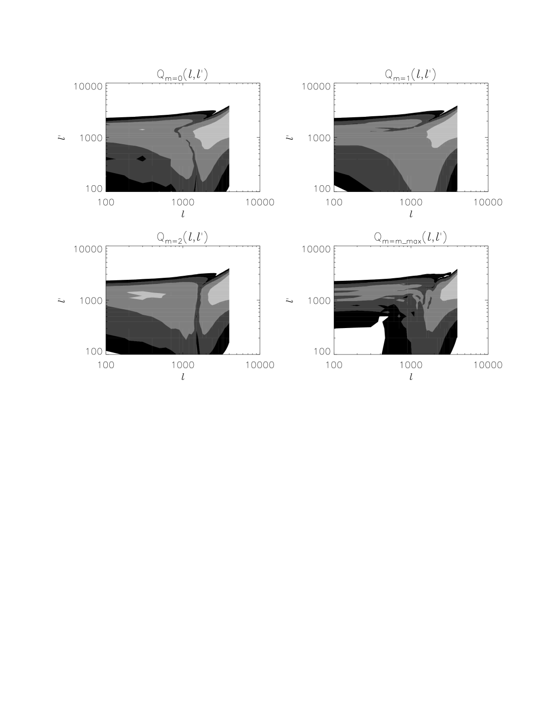
Figure 1: Contour plots of Qm(,).subscript𝑄𝑚superscriptQ_{m}(\ell,\ell^{\prime}). The levels denote the orders of magnitude as fractions of the maximum value, delimited by {1,101,102,103,104}1superscript101superscript102superscript103superscript104\{1,10^{-1},10^{-2},10^{-3},10^{-4}\} from the lightest to the darkest shade. Here mmax=16,subscript𝑚𝑚𝑎𝑥16m_{max}=16, max=4000subscript𝑚𝑎𝑥4000\ell_{max}=4000 for PLANCK noise at ν=143GHz.𝜈143GHz\nu=143\leavevmode\nobreak\ {\rm GHz}.

Refer to caption


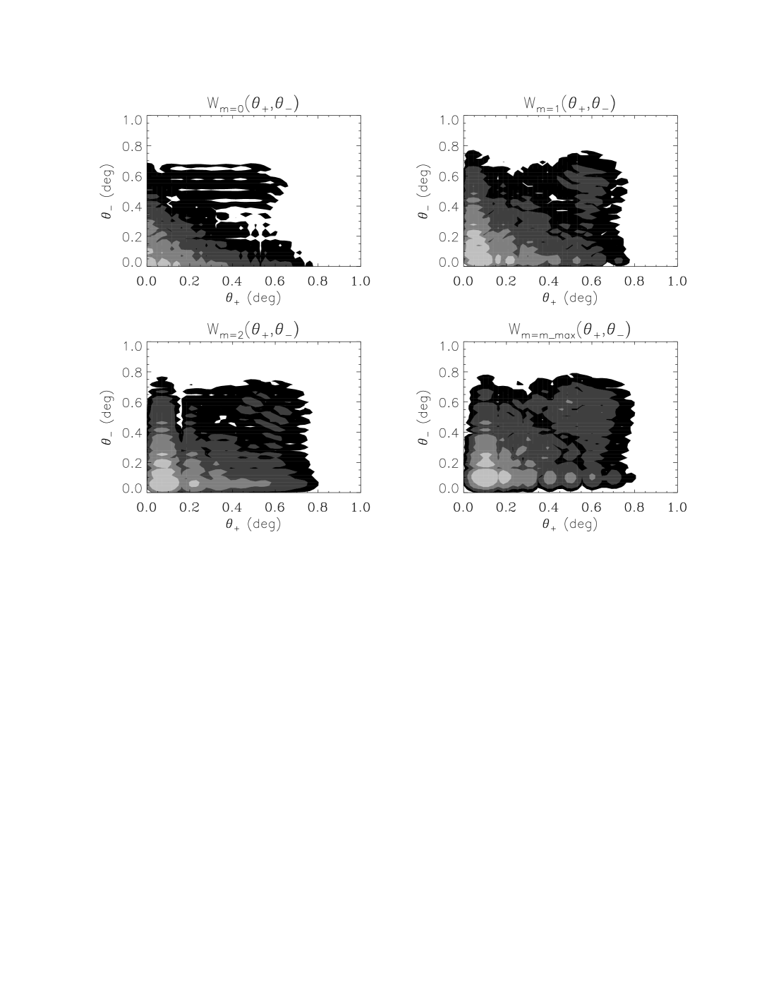
Figure 2: Contour plots of Wm(θ+,θ).subscript𝑊𝑚subscript𝜃subscript𝜃W_{m}(\theta_{+},\theta_{-}). The levels denote the orders of magnitude as fractions of the maximum value, delimited by {1,101,102,103,104}1superscript101superscript102superscript103superscript104\{1,10^{-1},10^{-2},10^{-3},10^{-4}\} from the lightest to the darkest shade. Here mmax=4,subscript𝑚𝑚𝑎𝑥4m_{max}=4, max=4000subscript𝑚𝑎𝑥4000\ell_{max}=4000 for no detector noise.

Refer to caption

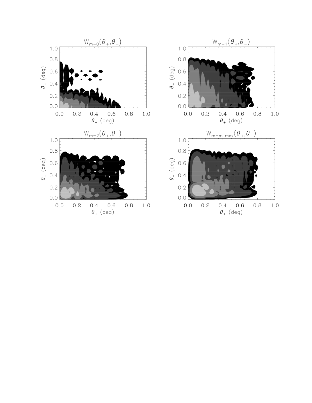
Figure 3: Contour plots of Wm(θ+,θ).subscript𝑊𝑚subscript𝜃subscript𝜃W_{m}(\theta_{+},\theta_{-}). The levels denote the orders of magnitude as fractions of the maximum value, delimited by {1,101,102,103,104}1superscript101superscript102superscript103superscript104\{1,10^{-1},10^{-2},10^{-3},10^{-4}\} from the lightest to the darkest shade. Here mmax=4,subscript𝑚𝑚𝑎𝑥4m_{max}=4, max=4000subscript𝑚𝑎𝑥4000\ell_{max}=4000 for PLANCK noise at ν=143GHz.𝜈143GHz\nu=143\leavevmode\nobreak\ {\rm GHz}.

Two parameters that we need to define for the computation of the kernel that affect the reconstruction of the lensing convergence are the kernel extent in \ell space, max,subscript𝑚𝑎𝑥\ell_{max}, and the number of eigenfunctions at which we will truncate the series in m,𝑚m, mmax.subscript𝑚𝑚𝑎𝑥m_{max}. Since the kernel is computed from the lensed map, the value of maxsubscript𝑚𝑎𝑥\ell_{max} should be determined by the range in \ell space that the experiment can probe before the beam and noise cut off the signal. We thus set maxsubscript𝑚𝑎𝑥\ell_{max} equal to the higher \ell moment that we use to synthesise the maps, i.e. max=4000.subscript𝑚𝑎𝑥4000\ell_{max}=4000. This is also consistent with the value read off of Qm(,)subscript𝑄𝑚superscriptQ_{m}(\ell,\ell^{\prime}) which we plot in Fig. 1. 333The small scale structure seen in Fig. 1 is likely numerical noise due to the discretization. Various tests that we tried seem to indicate that the quality of the lensing reconstruction is not significantly affected by this small scale structure. Nevertheless, we plan to improve the numerical calculation of the kernel and its transformation in future higher precision studies. We have tried using higher values for maxsubscript𝑚𝑎𝑥\ell_{max} and found that neither the kernel nor the reconstructed power spectra changed significantly due to the fact that most of the lensing information is accessed around the beam scale. In the absence of detector noise, the kernel is displaced to higher values of \ell and ,superscript\ell^{\prime}, up to the chosen max.subscript𝑚𝑎𝑥\ell_{max}. To fix the value of mmaxsubscript𝑚𝑚𝑎𝑥m_{max} we compared the relative amplitude of each eigenfunction Wm(𝜽+,𝜽)subscript𝑊𝑚subscript𝜽subscript𝜽W_{m}(\boldsymbol{\theta}_{+},\boldsymbol{\theta}_{-}) and discarded those that were less than 1%percent11\% of the dominant m=0𝑚0m=0 eigenfunction. This corresponds to mmax=4.subscript𝑚𝑚𝑎𝑥4m_{max}=4.

For each experiment we generate Wm(θ+,θ)subscript𝑊𝑚subscript𝜃subscript𝜃W_{m}(\theta_{+},\theta_{-}) for the selected values of these two parameters. In Figs. 2 and 3 we show the contour plots of four eigenfunctions of the kernel in real space for the Designer and the Planck experiment respectively. From the plot of the m=0𝑚0m=0 eigenfunction (which we have found to dominate the lensing reconstruction) we read off the value for the spatial extent of the kernel θmax,subscript𝜃𝑚𝑎𝑥\theta_{max}, used in the convolution routine to compute the convergence map. In harmonic space the kernel peaks at the scale of the beam but has support at smaller \ell values. The spatial extent of the kernel is thus larger than the beam scale and scales roughly linearly with the beam size. We observe that the kernel is compact and extends only up to 0.70superscript0.700.70^{\circ} and 0.60superscript0.600.60^{\circ} at the 1%percent11\% level in the absence and in the presence of detector noise respectively. In practice, the cut-off in the kernel was tested by comparing the power spectrum of the convergence map reconstructed for different values of θmax.subscript𝜃𝑚𝑎𝑥\theta_{max}. For each experiment, we verified that increasing the value of θmaxsubscript𝜃𝑚𝑎𝑥\theta_{max} beyond 0.35superscript0.350.35^{\circ} did not improve the reconstruction of the power spectrum, whereas reducing the value of θmaxsubscript𝜃𝑚𝑎𝑥\theta_{max} below 0.35superscript0.350.35^{\circ} degraded the reconstruction. We thus set θmax=0.35.subscript𝜃𝑚𝑎𝑥superscript0.35\theta_{max}=0.35^{\circ}.

IV.2 Compute the convergence map

We compute the estimator by convolving the kernel with the lensed CMB map according to Eqn. (40). We implement the convolution using the discrete version of this equation as follows

κ0(𝜽=0)subscript𝜅0𝜽0\displaystyle\kappa_{0}(\boldsymbol{\theta}=0) =\displaystyle= m=mmaxmmaxθ+xθ+yθxθyexp[imarctan(θ+yθyθ+xθx)]superscriptsubscript𝑚subscript𝑚𝑚𝑎𝑥subscript𝑚𝑚𝑎𝑥subscriptsubscript𝜃𝑥subscriptsubscript𝜃𝑦subscriptsubscript𝜃𝑥subscriptsubscript𝜃𝑦𝑖𝑚subscript𝜃𝑦subscript𝜃𝑦subscript𝜃𝑥subscript𝜃𝑥\displaystyle\sum_{m=-m_{max}}^{m_{max}}\leavevmode\nobreak\ \sum_{\theta_{+x}}\sum_{\theta_{+y}}\sum_{\theta_{-x}}\sum_{\theta_{-y}}\leavevmode\nobreak\ \exp\left[im\arctan\left({{\theta_{+y}-\theta_{-y}}\over{\theta_{+x}-\theta_{-x}}}\right)\right] (45)
×T~(θ+x+θx,θ+y+θy)T~(θ+xθx,θ+yθy)absent~𝑇subscript𝜃𝑥subscript𝜃𝑥subscript𝜃𝑦subscript𝜃𝑦~𝑇subscript𝜃𝑥subscript𝜃𝑥subscript𝜃𝑦subscript𝜃𝑦\displaystyle\times\tilde{T}(\theta_{+x}+\theta_{-x},\theta_{+y}+\theta_{-y})\leavevmode\nobreak\ \tilde{T}(\theta_{+x}-\theta_{-x},\theta_{+y}-\theta_{-y})
×Wm(θ+x2+θ+y2,θx2+θy2).absentsubscript𝑊𝑚superscriptsubscript𝜃𝑥2superscriptsubscript𝜃𝑦2superscriptsubscript𝜃𝑥2superscriptsubscript𝜃𝑦2\displaystyle\times W_{m}\left(\sqrt{\theta_{+x}^{2}+\theta_{+y}^{2}},\sqrt{\theta_{-x}^{2}+\theta_{-y}^{2}}\right).

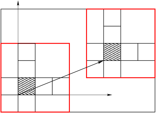
The size of the kernel determines the extent of the temperature map over which the convolution is computed. Since the temperature map is evaluated at the sum and difference of the contributing pixels, we need a region of the temperature map that is four times the length of the kernel to compute the convolution (see Fig. 4). At an arbitrary point 𝜽=(θ0x,θ0y)𝜽subscript𝜃0𝑥subscript𝜃0𝑦\boldsymbol{\theta}=(\theta_{0x},\theta_{0y}) the convergence is given by the estimator at the origin translated by the vector 𝜽.𝜽\boldsymbol{\theta}.
Refer to caption

𝜽subscript𝜽\boldsymbol{\theta}_{-}𝜽0subscript𝜽0\boldsymbol{\theta}_{0}𝜽+subscript𝜽\boldsymbol{\theta}_{+}

Figure 4: Relative sizes in the reconstruction of the convergence map. The outer black square represents the map and the inner, dashed square centred at the origin represents the kernel. The red square around the kernel encompasses the points on the map which contribute to the convergence on the point where the kernel is centred. The kernel moves over the map by successive translations indicated by the vector 𝜽0.subscript𝜽0\boldsymbol{\theta}_{0}. At the new centre, a new red square is defined. This procedure is repeated until the red square reaches the boundary of the map.

We then average the reconstructed convergence map over all pixels to extract the zero mode, which is then subtracted from the map as discussed in the text following Eqn. (42). Finally we subtract the convergence power spectrum of a Monte Carlo realization of one hundred unlensed CMB maps from the convergence power spectrum of the lensing potential, thus removing the gaussian bias from the estimated power spectrum. Our implementation of the real space estimator takes a little over one minute in total on a desktop computer, including the calculation of the kernel (about 30 sec) and the reconstruction of the convergence map (about 40 sec). This is about six times the time that the harmonic space implementation takes to reconstruct the lensing field.

V Results and Discussion

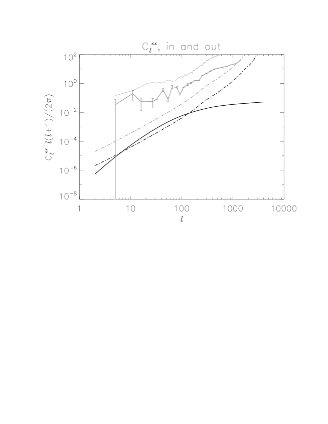
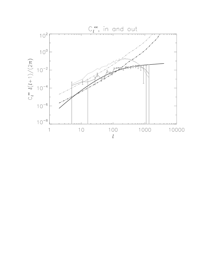
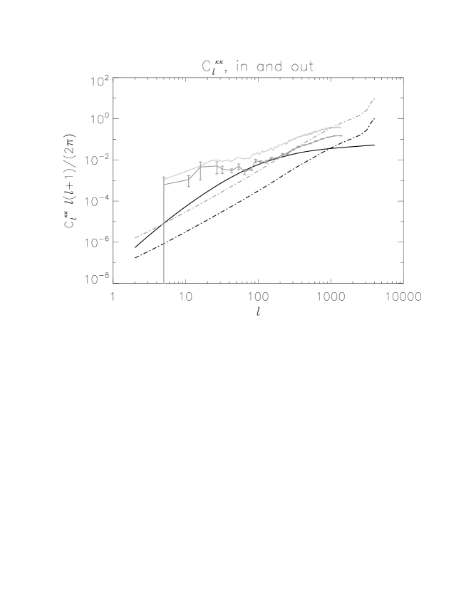
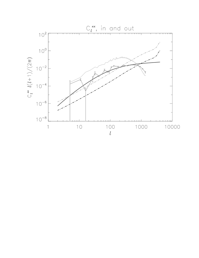
For each experiment we plot the output power spectrum Cκoutκoutsuperscriptsubscript𝐶subscript𝜅𝑜𝑢𝑡subscript𝜅𝑜𝑢𝑡C_{\ell}^{\kappa_{out}\kappa_{out}}, both before (light grey solid line) and after (dark grey solid line) the removal of the bias, against the input power spectrum Cκinκinsuperscriptsubscript𝐶subscript𝜅𝑖𝑛subscript𝜅𝑖𝑛C_{\ell}^{\kappa_{in}\kappa_{in}} (black solid line). In Figs. 5 and 6 we plot the reconstructed power spectra for the Designer and the Planck experiment respectively. We also plot the variance of the estimator Var[κ^0()]Vardelimited-[]subscript^𝜅0bold-ℓ{\rm Var}[\hat{\kappa}_{0}(\boldsymbol{\ell})] (black dot-dashed line) as well as Var[κ^0()]/fskyVardelimited-[]subscript^𝜅0bold-ℓsubscript𝑓𝑠𝑘𝑦{\rm Var}[\hat{\kappa}_{0}(\boldsymbol{\ell})]/f_{sky} (grey dot-dashed line) as an auxiliary tool for visualization. The error bars on the recovered power spectra are computed from the standard deviation of the reconstructed power spectrum, binned over logarithmically spaced intervals in \ell space and added in quadrature. The variance of the reconstructed power spectrum encompasses both the variance of the optimal estimator and the average value of the convergence fluctuation in the map, weighted by the fraction of the area of the sky covered by the patch, fsky,subscript𝑓𝑠𝑘𝑦f_{sky}, as follows tegmark

Var[Cκ0κ0]1fsky(Var[κ^0()]+Clκ0κ0)2.Vardelimited-[]superscriptsubscript𝐶subscript𝜅0subscript𝜅01subscript𝑓𝑠𝑘𝑦superscriptVardelimited-[]subscript^𝜅0bold-ℓsuperscriptsubscript𝐶𝑙subscript𝜅0subscript𝜅02\displaystyle{\rm Var}[C_{\ell}^{\kappa_{0}\kappa_{0}}]\approx{1\over{\ell\leavevmode\nobreak\ f_{sky}}}\left({\rm Var}[\hat{\kappa}_{0}(\boldsymbol{\ell})]+C_{l}^{\kappa_{0}\kappa_{0}}\right)^{2}. (46)

We observe that the degree of recovery of the input power spectra is not the same throughout the interval in .\ell. In particular, at small \ell the cosmic variance dominates the error of the reconstruction, whereas at large \ell the variance of the estimator takes over. The region where Cκinκin>Var[κ^0()]superscriptsubscript𝐶subscript𝜅𝑖𝑛subscript𝜅𝑖𝑛Vardelimited-[]subscript^𝜅0bold-ℓC_{\ell}^{\kappa_{in}\kappa_{in}}>{\rm Var}[\hat{\kappa}_{0}(\boldsymbol{\ell})] indicates the interval in \ell where the lensing potential can in theory be mapped. Accordingly, this is also the region where the reconstructed convergence power spectra tracks more closely the input power spectrum. Also visible are the fluctuations in the recovered power spectrum which arise from the subtraction of the noise bias term estimated from a finite number of realizations of the unlensed CMB map.

For the Planck experiment, using the real space implementation we achieve a reasonable reconstruction of the input power spectrum in the interval where the input signal is larger than the variance of the estimator, although on smaller scales, >600,600\ell>600, there is a decrease in the recovered power. Comparing the reconstructed power spectra for the Designer and Planck experiments we observe that the real space implementation is fairly insensitive to the detector noise and returns a reconstruction consistent with the input power spectrum. We can understand these results as follows.
Refer to caption Refer to caption

Figure 5: Mean square of the convergence map reconstructed with the harmonic space estimator (left panel) and the real space estimator (right panel). The smooth black curve is the input power spectrum. The light grey and dark grey solid lines are the output power spectra before and after the removal of the bias respectively. The error bars measure the total standard deviation binned over logarithmically spaced intervals in .\ell. Here θfwhm=7.8,subscript𝜃𝑓𝑤𝑚superscript7.8\theta_{fwhm}=7.8^{\prime}, FOVmap=66.6𝐹𝑂subscript𝑉𝑚𝑎𝑝superscript66.6FOV_{map}=66.6^{\circ} and mmax=4,subscript𝑚𝑚𝑎𝑥4m_{max}=4, max=4000subscript𝑚𝑎𝑥4000\ell_{max}=4000 for no detector noise.

Refer to caption Refer to caption


Figure 6: Mean square of the convergence map reconstructed with the harmonic space estimator (left panel) and the real space estimator (right panel). The smooth black curve is the input power spectrum. The light grey and dark grey solid lines are the output power spectra before and after the removal of the bias respectively. The error bars measure the total standard deviation binned over logarithmically spaced intervals in .\ell. Here θfwhm=7.8,subscript𝜃𝑓𝑤𝑚superscript7.8\theta_{fwhm}=7.8^{\prime}, FOVmap=66.6,𝐹𝑂subscript𝑉𝑚𝑎𝑝superscript66.6FOV_{map}=66.6^{\circ}, and mmax=4,subscript𝑚𝑚𝑎𝑥4m_{max}=4, max=4000subscript𝑚𝑎𝑥4000\ell_{max}=4000 for PLANCK noise at ν=143GHz.𝜈143GHz\nu=143\leavevmode\nobreak\ {\rm GHz}.

As attested by the power spectra of the maps reconstructed with the real space estimator, there is a loss of power at small scales beginning around the angular scale corresponding to the size of the kernel. This loss of power is a consequence of averaging modes smaller than the finite extent of the kernel and hence is an intrinsic constraint of the real space implementation. This intrinsic constraint, studied in more detail in Ref. bucher2010 , can be overcome by shrinking the extent of the kernel in real space, which can be achieved with a smaller beam and detector noise, thereby moving the support for the kernel to larger .\ell. The \ell interval over which the power spectrum can be recovered by the real space estimator is determined by the characteristic lengths of the map and the kernel as follows. The lower \ell limit is determined by the size of the map, since it measures the longest wavelength mode that can be enclosed within the size of the map. The upper \ell limit is determined by the size of the kernel, since it measures the smallest wavelength mode that the kernel can probe, below which there is a loss of power due to the averaging of modes smaller than the size of the kernel. Within this \ell range, the real space estimator seems to perform fairly well both in the absence and in the presence of detector noise. Note that the \ell range for a reasonable reconstruction with the harmonic space estimator is wider, being limited at higher \ell by the angular scale corresponding to the beam size, since this is the scale which constrains the action of the kernel in harmonic space.

Comparing the reconstructed power spectra in the absence and in the presence of detector noise, we observe that the real space estimator appears to be insensitive to the experimental noise. This is because the estimate of the convergence in each pixel is given by the sum of the product of pairs of neighbouring pixels weighted by the kernel. As a result, the noise, being independent in each pixel, is averaged out. To substantiate this result, we reconstructed the convergence map from a pure white noise input map using the real space estimator and the harmonic space estimator. In Fig. 7 we observe that the power spectrum recovered by the real space estimator is about seven orders of magnitude smaller than the input power spectrum, whereas the power spectrum recovered by the harmonic space estimator is comparable to the input power spectrum.

Despite our attempt to remove the CMB and the detector noise bias from the reconstructed convergence power spectrum, there still remains a bias in the harmonic space implementation, as observed in Figs. 5 and 6. This bias presumably arises from a coupling between unlensed temperature modes due to the finite size of the map, providing an additional source of lensing which we have not treated here. This mode coupling is absent in the reconstruction over the full sky inpaint . The real space implementation appears to be insensitive to this bias.

Refer to caption


Figure 7: Mean square of the convergence map reconstructed with the harmonic space estimator (light grey line) and the real space estimator (dark grey line) from a pure white noise map. The grey solid lines are the output power spectra whereas the smooth black curve is the input power spectrum. Here θfwhm=7.8,subscript𝜃𝑓𝑤𝑚superscript7.8\theta_{fwhm}=7.8^{\prime}, FOVmap=66.6,𝐹𝑂subscript𝑉𝑚𝑎𝑝superscript66.6FOV_{map}=66.6^{\circ}, and mmax=4,subscript𝑚𝑚𝑎𝑥4m_{max}=4, max=4000subscript𝑚𝑎𝑥4000\ell_{max}=4000 for PLANCK noise at ν=143GHz.𝜈143GHz\nu=143\leavevmode\nobreak\ {\rm GHz}.

VI Summary and future work

In this paper we implemented a new estimator of the convergence field for the extraction of the lensing potential from CMB maps. Our interest was in reconstructing the convergence field from CMB maps from which contaminants, such as point sources and the SZ effect, had previously been removed using multi-frequency information.

The new estimator acts locally in real space, thus being able to treat the excision of pixels and nonuniform sky coverage in a flexible manner. We implemented the estimator on two experimental setups, one without and one with detector noise, based on the specifications of PLANCK for the ν=143GHz𝜈143GHz\nu=143\leavevmode\nobreak\ {\rm GHz} channel. For comparison of the performance of the new estimator, we also implemented the conventional estimator which acts in harmonic space. From the two experiments we learned that by increasing the range of the kernel in \ell space, and consequently reducing its range in θ𝜃\theta space, we improve the reconstruction of the power spectrum at small scales. The finite extent of the kernel is a desirable property of the proposed estimator, since in theory it allows the reconstruction of the lensing convergence, manifested essentially at very small scales, from a small map of the sky as long as the kernel probes sufficiently small angular scales. Even though there is a loss of power on scales smaller than the finite extent of the kernel, this effect could be studied using simulations to determine a form factor that could be applied to correct the loss of power bucher2010 . We also observed that although the real space estimator is limited, in a statistical sense, to be as good as the harmonic space estimator, it has the advantage over the harmonic space estimator of being less sensitive to white noise. In practice, however, CMB experiments have to deal with correlated noise, which will pose as much of a challenge to the real space estimator as to the harmonic space estimator, most likely requiring the construction of a more carefully designed kernel in harmonic space that downweights the correlated modes before transforming to real space.

On the basis of the results presented here, we envisage two follow-up studies. In the first study we intend to optimize the current implementation of the real space estimator to use a kernel capable of probing smaller angular scales in the reconstruction of the lensing convergence, as we would expect for the ACT and SPT experiments. As we have demonstrated, the real space estimator can be applied to small patches of sky without incurring in the serious spectral leakage that affects the harmonic space estimator on rectangular, rather than torodial, domains in the presence of red spectra. In real space, the local filter acts up to a kernel length away from the edge of the map without leakage of power. We also intend to study the effect of a mask due to the excision of bad pixels, e.g. arising from the removal of bright point sources, that can cause aliasing of power from large scales to small scales. Inpainting has been proposed as a means of interpolating across masked regions that preserves the statistical properties of the map inpaint , so we plan to investigate how sensitive the real space estimator is to complex masks with and without the use of such techniques.

A straightforward extension will be to develop the analogous estimator for the shear components of the convergence tensor and work out how to combine the different components for the reconstruction of the lensing potential. Since the shear components do not contain the =00\ell=0 mode, the corresponding estimators will be less sensitive to a bias. The dilatation and shear components provide complementary information on the lensing potential but are not independent, being related by consistency conditions that are algebraic in harmonic space. Since these components probe the monopole and quadrupole sectors respectively, the noise associated with these components will be uncorrelated and the reconstruction can be harmonized, with the noise being reduced via inverse variance weighting of these components. This point is discussed in more detail in Ref. bucher2010 .

In the second study we intend to extend the implementation of the real space estimator to CMB polarisation so as to optimize the reconstruction of the lensing potential from the PLANCK data.

Acknowledgments

The authors are supported by the South African National Research Foundation. The authors acknowledge the use of codes by M Bucher and the use of CAMB camb . The authors also thank M Bucher, S Das, D Spergel, B Sherwin and M Remazeilles for useful discussions, as well as the anonymous referee for a number of useful comments. CSC also acknowledges the hospitality of the Astrophysical Sciences Department, Princeton University.

Appendix A Derivation of the harmonic space estimator

In this Appendix we derive the optimal estimator for the lensing potential in harmonic space. From Eqn. (16) a crude estimator for the lensing potential would be the 0bold-ℓ0\boldsymbol{\ell}\not=0 term

ψ^(,)=1(2π)2T~()T~()[C+()C||].^𝜓bold-ℓsuperscriptbold-ℓ1superscript2𝜋2~𝑇superscriptbold-ℓ~𝑇bold-ℓsuperscriptbold-ℓdelimited-[]bold-ℓsuperscriptbold-ℓsubscript𝐶superscriptbold-ℓbold-ℓsuperscriptbold-ℓsubscript𝐶bold-ℓsuperscriptbold-ℓ\displaystyle\hat{\psi}(\boldsymbol{\ell},\boldsymbol{\ell}^{\prime})={1\over(2\pi)^{2}}{\tilde{T}(\boldsymbol{\ell}^{\prime})\leavevmode\nobreak\ \tilde{T}(\boldsymbol{\ell}-\boldsymbol{\ell}^{\prime})\over\left[\boldsymbol{\ell}\cdot\boldsymbol{\ell}^{\prime}\leavevmode\nobreak\ C_{\ell^{\prime}}+\boldsymbol{\ell}\cdot(\boldsymbol{\ell}-\boldsymbol{\ell}^{\prime})\leavevmode\nobreak\ C_{|\boldsymbol{\ell}-\boldsymbol{\ell}^{\prime}|}\right]}. (47)

This way we would be estimating the anisotropic component of the convergence which is due to the lensing potential only, i.e. without the isotropic zero mode.

We now seek for the optimal combination

ψ^()=d2(2π)2ψ^(,)G(,),^𝜓bold-ℓsuperscript𝑑2superscriptbold-ℓsuperscript2𝜋2^𝜓bold-ℓsuperscriptbold-ℓ𝐺bold-ℓsuperscriptbold-ℓ\displaystyle\hat{\psi}(\boldsymbol{\ell})=\int{d^{2}\boldsymbol{\ell}^{\prime}\over(2\pi)^{2}}\leavevmode\nobreak\ \hat{\psi}(\boldsymbol{\ell},\boldsymbol{\ell}^{\prime})\leavevmode\nobreak\ G(\boldsymbol{\ell},\boldsymbol{\ell}^{\prime}), (48)

where the optimal weights G(,)𝐺bold-ℓsuperscriptbold-ℓG(\boldsymbol{\ell},\boldsymbol{\ell}^{\prime}) are given by

G(,)=1σψ^(,)2[d2(2π)2d2(2π)21σψ^(,)2]1𝐺bold-ℓsuperscriptbold-ℓ1superscriptsubscript𝜎^𝜓bold-ℓsuperscriptbold-ℓ2superscriptdelimited-[]superscript𝑑2bold-ℓsuperscript2𝜋2superscript𝑑2superscriptbold-ℓsuperscript2𝜋21superscriptsubscript𝜎^𝜓bold-ℓsuperscriptbold-ℓ21\displaystyle G(\boldsymbol{\ell},\boldsymbol{\ell}^{\prime})={1\over\sigma_{\hat{\psi}(\boldsymbol{\ell},\boldsymbol{\ell}^{\prime})}^{2}}\left[\int{d^{2}\boldsymbol{\ell}\over(2\pi)^{2}}\int{d^{2}\boldsymbol{\ell}^{\prime}\over(2\pi)^{2}}{1\over\sigma_{\hat{\psi}(\boldsymbol{\ell},\boldsymbol{\ell}^{\prime})}^{2}}\right]^{-1} (49)

so as to minimize the variance, and are such that

d2(2π)2d2(2π)2G(,)=1superscript𝑑2bold-ℓsuperscript2𝜋2superscript𝑑2superscriptbold-ℓsuperscript2𝜋2𝐺bold-ℓsuperscriptbold-ℓ1\displaystyle\int{d^{2}\boldsymbol{\ell}\over(2\pi)^{2}}\int{d^{2}\boldsymbol{\ell}^{\prime}\over(2\pi)^{2}}\leavevmode\nobreak\ G(\boldsymbol{\ell},\boldsymbol{\ell}^{\prime})=1 (50)

so as to make the estimator unbiased <ψ^(,)>=ψ().expectation^𝜓bold-ℓsuperscriptbold-ℓ𝜓bold-ℓ\bigl{<}\hat{\psi}(\boldsymbol{\ell},\boldsymbol{\ell}^{\prime})\bigr{>}=\psi(\boldsymbol{\ell}). Here σψ^(,)2superscriptsubscript𝜎^𝜓bold-ℓsuperscriptbold-ℓ2\sigma_{\hat{\psi}(\boldsymbol{\ell},\boldsymbol{\ell}^{\prime})}^{2} is the variance of ψ^(,)^𝜓bold-ℓsuperscriptbold-ℓ\hat{\psi}(\boldsymbol{\ell},\boldsymbol{\ell}^{\prime}) which for the case that ψ()𝜓bold-ℓ\psi(\boldsymbol{\ell}) is centred at zero becomes

σψ^(,)2superscriptsubscript𝜎^𝜓bold-ℓsuperscriptbold-ℓ2\displaystyle\sigma_{\hat{\psi}(\boldsymbol{\ell},\boldsymbol{\ell}^{\prime})}^{2} =\displaystyle= (ψ^(1,1)ψ(1))(ψ^(2,2)ψ(2))delimited-⟨⟩^𝜓subscriptbold-ℓ1subscriptsuperscriptbold-ℓ1𝜓subscriptbold-ℓ1superscript^𝜓subscriptbold-ℓ2subscriptsuperscriptbold-ℓ2𝜓subscriptbold-ℓ2\displaystyle\left<\left(\hat{\psi}(\boldsymbol{\ell}_{1},\boldsymbol{\ell}^{\prime}_{1})-\psi(\boldsymbol{\ell}_{1})\right)\left(\hat{\psi}(\boldsymbol{\ell}_{2},\boldsymbol{\ell}^{\prime}_{2})-\psi(\boldsymbol{\ell}_{2})\right)^{\ast}\right> (51)
=\displaystyle= 1(2π)4T~(1)T~(11)T~(2)T~(22)1superscript2𝜋4delimited-⟨⟩~𝑇subscriptsuperscriptbold-ℓ1~𝑇subscriptbold-ℓ1subscriptsuperscriptbold-ℓ1superscript~𝑇subscriptsuperscriptbold-ℓ2superscript~𝑇subscriptbold-ℓ2subscriptsuperscriptbold-ℓ2\displaystyle{1\over(2\pi)^{4}}\left<\tilde{T}(\boldsymbol{\ell}^{\prime}_{1})\leavevmode\nobreak\ \tilde{T}(\boldsymbol{\ell}_{1}-\boldsymbol{\ell}^{\prime}_{1})\leavevmode\nobreak\ \tilde{T}^{\ast}(\boldsymbol{\ell}^{\prime}_{2})\leavevmode\nobreak\ \tilde{T}^{\ast}(\boldsymbol{\ell}_{2}-\boldsymbol{\ell}^{\prime}_{2})\right> (53)
×1[11C1+1(11)C|11|]1[22C2+2(22)C|22|]absent1delimited-[]subscriptbold-ℓ1subscriptsuperscriptbold-ℓ1subscript𝐶subscriptsuperscript1subscriptbold-ℓ1subscriptbold-ℓ1subscriptsuperscriptbold-ℓ1subscript𝐶subscriptbold-ℓ1subscriptsuperscriptbold-ℓ11delimited-[]subscriptbold-ℓ2subscriptsuperscriptbold-ℓ2subscript𝐶subscriptsuperscript2subscriptbold-ℓ2subscriptbold-ℓ2subscriptsuperscriptbold-ℓ2subscript𝐶subscriptbold-ℓ2subscriptsuperscriptbold-ℓ2\displaystyle\times{1\over\left[\boldsymbol{\ell}_{1}\cdot\boldsymbol{\ell}^{\prime}_{1}\leavevmode\nobreak\ C_{\ell^{\prime}_{1}}+\boldsymbol{\ell}_{1}\cdot(\boldsymbol{\ell}_{1}-\boldsymbol{\ell}^{\prime}_{1})\leavevmode\nobreak\ C_{|\boldsymbol{\ell}_{1}-\boldsymbol{\ell}^{\prime}_{1}|}\right]}{1\over\left[\boldsymbol{\ell}_{2}\cdot\boldsymbol{\ell}^{\prime}_{2}\leavevmode\nobreak\ C_{\ell^{\prime}_{2}}+\boldsymbol{\ell}_{2}\cdot(\boldsymbol{\ell}_{2}-\boldsymbol{\ell}^{\prime}_{2})\leavevmode\nobreak\ C_{|\boldsymbol{\ell}_{2}-\boldsymbol{\ell}^{\prime}_{2}|}\right]}
=\displaystyle= 2δ(12)δ(12)C~1C~|11|[11C1+1(11)C|11|]2.2𝛿subscriptbold-ℓ1subscriptbold-ℓ2𝛿subscriptsuperscriptbold-ℓ1subscriptsuperscriptbold-ℓ2subscript~𝐶subscriptsuperscript1subscript~𝐶subscriptbold-ℓ1subscriptsuperscriptbold-ℓ1superscriptdelimited-[]subscriptbold-ℓ1subscriptsuperscriptbold-ℓ1subscript𝐶subscriptsuperscript1subscriptbold-ℓ1subscriptbold-ℓ1subscriptsuperscriptbold-ℓ1subscript𝐶subscriptbold-ℓ1subscriptsuperscriptbold-ℓ12\displaystyle 2\leavevmode\nobreak\ \delta(\boldsymbol{\ell}_{1}-\boldsymbol{\ell}_{2})\leavevmode\nobreak\ \delta(\boldsymbol{\ell}^{\prime}_{1}-\boldsymbol{\ell}^{\prime}_{2}){{\tilde{C}_{\ell^{\prime}_{1}}\tilde{C}_{|\boldsymbol{\ell}_{1}-\boldsymbol{\ell}^{\prime}_{1}|}}\over{\left[\boldsymbol{\ell}_{1}\cdot\boldsymbol{\ell}^{\prime}_{1}\leavevmode\nobreak\ C_{\ell^{\prime}_{1}}+\boldsymbol{\ell}_{1}\cdot(\boldsymbol{\ell}_{1}-\boldsymbol{\ell}^{\prime}_{1})\leavevmode\nobreak\ C_{|\boldsymbol{\ell}_{1}-\boldsymbol{\ell}^{\prime}_{1}|}\right]^{2}}}. (54)

We then find for the optimal estimator that

ψ^()=𝒩d2(2π)2T~()T~()12C+()C||C~C~||,^𝜓bold-ℓsubscript𝒩superscript𝑑2superscriptbold-ℓsuperscript2𝜋2~𝑇superscriptbold-ℓ~𝑇bold-ℓsuperscriptbold-ℓ12bold-ℓsuperscriptbold-ℓsubscript𝐶superscriptbold-ℓbold-ℓsuperscriptbold-ℓsubscript𝐶bold-ℓsuperscriptbold-ℓsubscript~𝐶superscriptsubscript~𝐶bold-ℓsuperscriptbold-ℓ\displaystyle\hat{\psi}(\boldsymbol{\ell})=\mathcal{N_{\ell}}\int{d^{2}\boldsymbol{\ell}^{\prime}\over(2\pi)^{2}}\leavevmode\nobreak\ \tilde{T}(\boldsymbol{\ell}^{\prime})\leavevmode\nobreak\ \tilde{T}(\boldsymbol{\ell}-\boldsymbol{\ell}^{\prime})\leavevmode\nobreak\ {1\over 2}{{\boldsymbol{\ell}\cdot\boldsymbol{\ell}^{\prime}\leavevmode\nobreak\ C_{\ell^{\prime}}+\boldsymbol{\ell}\cdot(\boldsymbol{\ell}-\boldsymbol{\ell}^{\prime})\leavevmode\nobreak\ C_{|\boldsymbol{\ell}-\boldsymbol{\ell}^{\prime}|}}\over\tilde{C}_{\ell^{\prime}}\tilde{C}_{|\boldsymbol{\ell}-\boldsymbol{\ell}^{\prime}|}}, (55)

where

1𝒩=d2(2π)212[C+()C||]2C~C~||.1subscript𝒩superscript𝑑2superscriptbold-ℓsuperscript2𝜋212superscriptdelimited-[]bold-ℓsuperscriptbold-ℓsubscript𝐶superscriptbold-ℓbold-ℓsuperscriptbold-ℓsubscript𝐶bold-ℓsuperscriptbold-ℓ2subscript~𝐶superscriptsubscript~𝐶bold-ℓsuperscriptbold-ℓ\displaystyle{1\over\mathcal{N}_{\ell}}=\int{d^{2}\boldsymbol{\ell}^{\prime}\over(2\pi)^{2}}\leavevmode\nobreak\ {1\over 2}{{[\boldsymbol{\ell}\cdot\boldsymbol{\ell}^{\prime}\leavevmode\nobreak\ C_{\ell^{\prime}}+\boldsymbol{\ell}\cdot(\boldsymbol{\ell}-\boldsymbol{\ell}^{\prime})\leavevmode\nobreak\ C_{|\boldsymbol{\ell}-\boldsymbol{\ell}^{\prime}|}]^{2}}\over{\tilde{C}_{\ell^{\prime}}\leavevmode\nobreak\ \tilde{C}_{|\boldsymbol{\ell}-\boldsymbol{\ell}^{\prime}|}}}. (56)

Note that the calculation of the variance presupposes a prior knowledge of the unlensed power spectrum of the temperature anisotropies. Here we use the same TT𝑇𝑇TT power spectrum that we use for the synthesis of the CMB map.

The error associated with the reconstruction of the lensing potential with this estimator is given by the variance of the estimator. We can identify the variance of the estimator with the power spectrum of the estimator as follows σψ^(,)2=<ψ^(1,1)ψ^(2,2)>=(2π)2δ(12)δ(12)Var[ψ^(,)].superscriptsubscript𝜎^𝜓bold-ℓsuperscriptbold-ℓ2expectation^𝜓subscriptbold-ℓ1subscriptsuperscriptbold-ℓ1superscript^𝜓subscriptbold-ℓ2subscriptsuperscriptbold-ℓ2superscript2𝜋2𝛿subscriptbold-ℓ1subscriptbold-ℓ2𝛿subscriptsuperscriptbold-ℓ1subscriptsuperscriptbold-ℓ2Vardelimited-[]^𝜓bold-ℓsuperscriptbold-ℓ\sigma_{\hat{\psi}(\boldsymbol{\ell},\boldsymbol{\ell}^{\prime})}^{2}=\bigl{<}\hat{\psi}(\boldsymbol{\ell}_{1},\boldsymbol{\ell}^{\prime}_{1})\leavevmode\nobreak\ \hat{\psi}^{\ast}(\boldsymbol{\ell}_{2},\boldsymbol{\ell}^{\prime}_{2})\bigr{>}=(2\pi)^{2}\leavevmode\nobreak\ \delta(\boldsymbol{\ell}_{1}-\boldsymbol{\ell}_{2})\leavevmode\nobreak\ \delta(\boldsymbol{\ell}^{\prime}_{1}-\boldsymbol{\ell}^{\prime}_{2})\leavevmode\nobreak\ {\rm Var}[\hat{\psi}(\boldsymbol{\ell},\boldsymbol{\ell}^{\prime})]. It follows that the variance of the optimal estimator is given by

σψ^()2=[d22(2π)2d21(2π)21σψ^(,)2]1=(2π)2δ(12)Var[ψ^()]subscriptsuperscript𝜎2^𝜓bold-ℓsuperscriptdelimited-[]superscript𝑑2subscriptsuperscriptbold-ℓ2superscript2𝜋2superscript𝑑2subscriptsuperscriptbold-ℓ1superscript2𝜋21superscriptsubscript𝜎^𝜓bold-ℓsuperscriptbold-ℓ21superscript2𝜋2𝛿subscriptbold-ℓ1subscriptbold-ℓ2Vardelimited-[]^𝜓bold-ℓ\displaystyle\sigma^{2}_{\hat{\psi}(\boldsymbol{\ell})}=\left[\int{d^{2}\boldsymbol{\ell}^{\prime}_{2}\over(2\pi)^{2}}\int{d^{2}\boldsymbol{\ell}^{\prime}_{1}\over(2\pi)^{2}}{1\over\sigma_{\hat{\psi}(\boldsymbol{\ell},\boldsymbol{\ell}^{\prime})}^{2}}\right]^{-1}=(2\pi)^{2}\leavevmode\nobreak\ \delta(\boldsymbol{\ell}_{1}-\boldsymbol{\ell}_{2})\leavevmode\nobreak\ {\rm Var}[\hat{\psi}(\boldsymbol{\ell})] (57)

where

Var[ψ^()]=[d2(2π)212[C+()C||]2C~C~||]1=𝒩.Vardelimited-[]^𝜓bold-ℓsuperscriptdelimited-[]superscript𝑑2superscriptbold-ℓsuperscript2𝜋212superscriptdelimited-[]bold-ℓsuperscriptbold-ℓsubscript𝐶superscriptbold-ℓbold-ℓsuperscriptbold-ℓsubscript𝐶bold-ℓsuperscriptbold-ℓ2subscript~𝐶superscriptsubscript~𝐶bold-ℓsuperscriptbold-ℓ1subscript𝒩\displaystyle{\rm Var}[\hat{\psi}(\boldsymbol{\ell})]=\left[\int{d^{2}\boldsymbol{\ell}^{\prime}\over(2\pi)^{2}}\leavevmode\nobreak\ {1\over 2}{{[\boldsymbol{\ell}\cdot\boldsymbol{\ell}^{\prime}\leavevmode\nobreak\ C_{\ell^{\prime}}+\boldsymbol{\ell}\cdot(\boldsymbol{\ell}-\boldsymbol{\ell}^{\prime})\leavevmode\nobreak\ C_{|\boldsymbol{\ell}-\boldsymbol{\ell}^{\prime}|}]^{2}}\over{\tilde{C}_{\ell^{\prime}}\leavevmode\nobreak\ \tilde{C}_{|\boldsymbol{\ell}-\boldsymbol{\ell}^{\prime}|}}}\right]^{-1}=\mathcal{N}_{\ell}. (58)

The variance gives an upper limit to the dispersion about the mean reconstructed map of the output maps reconstructed with the estimator from a finite sample of input synthesised maps, thus being a measure that can be used to validate the estimator.

The expression for the optimal estimator can most straightforwardly be modified to incorporate detector noise and finite beam width by replacing C~subscript~𝐶superscript\tilde{C}_{\ell^{\prime}} by C~+N.subscript~𝐶superscriptsubscript𝑁superscript\tilde{C}_{\ell^{\prime}}+N_{\ell^{\prime}}. The noise power spectrum Nsubscript𝑁N_{\ell} is given by the inverse-sum over the number of channels of the detector noise ni()subscript𝑛𝑖n_{i}(\ell) of each channel i𝑖i

N=(i=0𝚗𝚞𝚖_𝚌𝚑𝚊𝚗𝚗1ni())1.subscript𝑁superscriptsuperscriptsubscript𝑖0𝚗𝚞𝚖_𝚌𝚑𝚊𝚗𝚗1subscript𝑛𝑖1\displaystyle N_{\ell}=\left(\sum_{i=0}^{\tt num\_chann}{1\over n_{i}(\ell)}\right)^{-1}. (59)

The detector noise is modelled by a gaussian signal on the beam size and includes both the white noise amplitude and the beam profile attenuation factor as follows

ni()=(θfwhmiσpixi)2exp[(θfwhmi)2(+1)/(8ln2)].subscript𝑛𝑖superscriptsubscriptsubscript𝜃𝑓𝑤𝑚𝑖subscriptsubscript𝜎𝑝𝑖𝑥𝑖2superscriptsubscriptsubscript𝜃𝑓𝑤𝑚𝑖2182\displaystyle n_{i}(\ell)=\left({\theta_{fwhm}}_{i}{\sigma_{pix}}_{i}\right)^{2}\exp[({\theta_{fwhm}}_{i})^{2}\ell(\ell+1)/(8\ln 2)]. (60)

Here θfwhmisubscriptsubscript𝜃𝑓𝑤𝑚𝑖{\theta_{fwhm}}_{i} is the beam full-width at half-maximum of the beam and σpixisubscriptsubscript𝜎𝑝𝑖𝑥𝑖{\sigma_{pix}}_{i} is the white noise amplitude per beam width.

We can regard Nsubscript𝑁N_{\ell} as the total variance of a multiple sampling of size the number of channels, each sampling i𝑖i having variance ni().subscript𝑛𝑖n_{i}(\ell). Finally, the estimator for the lensing potential becomes

ψ^()=𝒩d2(2π)2T~()T~()12C+()C||[C~+N][C~||+N||],^𝜓bold-ℓsubscript𝒩superscript𝑑2superscriptbold-ℓsuperscript2𝜋2~𝑇superscriptbold-ℓ~𝑇bold-ℓsuperscriptbold-ℓ12bold-ℓsuperscriptbold-ℓsubscript𝐶superscriptbold-ℓbold-ℓsuperscriptbold-ℓsubscript𝐶bold-ℓsuperscriptbold-ℓdelimited-[]subscript~𝐶superscriptsubscript𝑁delimited-[]subscript~𝐶bold-ℓsuperscriptbold-ℓsubscript𝑁bold-ℓsuperscriptbold-ℓ\displaystyle\hat{\psi}(\boldsymbol{\ell})=\mathcal{N}_{\ell}\int{d^{2}\boldsymbol{\ell}^{\prime}\over(2\pi)^{2}}\leavevmode\nobreak\ \tilde{T}(\boldsymbol{\ell}^{\prime})\leavevmode\nobreak\ \tilde{T}(\boldsymbol{\ell}-\boldsymbol{\ell}^{\prime})\leavevmode\nobreak\ {1\over 2}{{\boldsymbol{\ell}\cdot\boldsymbol{\ell}^{\prime}\leavevmode\nobreak\ C_{\ell^{\prime}}+\boldsymbol{\ell}\cdot(\boldsymbol{\ell}-\boldsymbol{\ell}^{\prime})\leavevmode\nobreak\ C_{|\boldsymbol{\ell}-\boldsymbol{\ell}^{\prime}|}}\over{[\tilde{C}_{\ell^{\prime}}+N_{\ell}][\tilde{C}_{|\boldsymbol{\ell}-\boldsymbol{\ell}^{\prime}|}+N_{|\boldsymbol{\ell}-\boldsymbol{\ell}^{\prime}|}]}}, (61)

where

1𝒩=d2(2π)212[C+()C||]2[C~+N][C~||+N||].1subscript𝒩superscript𝑑2superscriptbold-ℓsuperscript2𝜋212superscriptdelimited-[]bold-ℓsuperscriptbold-ℓsubscript𝐶superscriptbold-ℓbold-ℓsuperscriptbold-ℓsubscript𝐶bold-ℓsuperscriptbold-ℓ2delimited-[]subscript~𝐶superscriptsubscript𝑁superscriptdelimited-[]subscript~𝐶bold-ℓsuperscriptbold-ℓsubscript𝑁bold-ℓsuperscriptbold-ℓ\displaystyle{1\over\mathcal{N}_{\ell}}=\int{d^{2}\boldsymbol{\ell}^{\prime}\over(2\pi)^{2}}\leavevmode\nobreak\ {1\over 2}{{[\boldsymbol{\ell}\cdot\boldsymbol{\ell}^{\prime}\leavevmode\nobreak\ C_{\ell^{\prime}}+\boldsymbol{\ell}\cdot(\boldsymbol{\ell}-\boldsymbol{\ell}^{\prime})\leavevmode\nobreak\ C_{|\boldsymbol{\ell}-\boldsymbol{\ell}^{\prime}|}]^{2}}\over{[\tilde{C}_{\ell^{\prime}}+N_{\ell^{\prime}}][\tilde{C}_{|\boldsymbol{\ell}-\boldsymbol{\ell}^{\prime}|}+N_{|\boldsymbol{\ell}-\boldsymbol{\ell}^{\prime}|}]}}. (62)

The estimator for the deflection angle 𝜶(𝜽)=ψ(𝜽)𝜶𝜽𝜓𝜽\boldsymbol{\alpha}(\boldsymbol{\theta})=\nabla\psi(\boldsymbol{\theta}) and the convergence κ0(𝜽)=2ψ(𝜽)/2subscript𝜅0𝜽superscript2𝜓𝜽2\kappa_{0}(\boldsymbol{\theta})=-\nabla^{2}\psi(\boldsymbol{\theta})/2 will be given respectively by the gradient and the divergence in real space of ψ^().^𝜓bold-ℓ\hat{\psi}(\boldsymbol{\ell}). In bold-ℓ\boldsymbol{\ell} space this amounts simply to

𝜶^()^𝜶bold-ℓ\displaystyle\hat{\boldsymbol{\alpha}}(\boldsymbol{\ell}) =\displaystyle= iψ^()𝑖bold-ℓ^𝜓bold-ℓ\displaystyle i\boldsymbol{\ell}\leavevmode\nobreak\ \hat{\psi}(\boldsymbol{\ell}) (63)
κ^0()subscript^𝜅0bold-ℓ\displaystyle\hat{\kappa}_{0}(\boldsymbol{\ell}) =\displaystyle= 2ψ^()superscript2^𝜓bold-ℓ\displaystyle\ell^{2}\leavevmode\nobreak\ \hat{\psi}(\boldsymbol{\ell}) (64)

with variances Var[α^()]=2Var[ψ^()]Vardelimited-[]^𝛼bold-ℓsuperscript2Vardelimited-[]^𝜓bold-ℓ{\rm Var}[\hat{\alpha}(\boldsymbol{\ell})]=\ell^{2}\leavevmode\nobreak\ {\rm Var}[\hat{\psi}(\boldsymbol{\ell})] and Var[κ^0()]=4Var[ψ^()]Vardelimited-[]subscript^𝜅0bold-ℓsuperscript4Vardelimited-[]^𝜓bold-ℓ{\rm Var}[\hat{\kappa}_{0}(\boldsymbol{\ell})]=\ell^{4}\leavevmode\nobreak\ {\rm Var}[\hat{\psi}(\boldsymbol{\ell})] respectively.

Appendix B Synthesis of the lensed CMB map

For the construction of the CMB map and the lensing map we used power spectra generated by CAMB camb , respectively the TT and the ψψ𝜓𝜓\psi\psi power spectra, on scales with 4000.4000\ell\leq 4000. Given the nature of the CMB lensing and the form of the data to be analysed, we will be working upon a square patch, thus bounded, of the unbounded celestial sphere. For a proper treatment of the boundaries of the patch, we must simulate the unboundedness of the sphere by implementing periodic boundary conditions. In order to reproduce periodic boundary conditions, we apodized the CMB map by smoothing to zero over a strip around the boundary with a given width fraction (in this case 0.10). The requirement of periodic boundary conditions makes the implementation of the quadratic estimator in harmonic space easier but is not necessary for the implementation of the real space estimator.

We then applied the lensing map to the CMB map to produce the lensed CMB map. This consisted of shifting the CMB map by the lensing potential assuming the Born approximation, as detailed in the Appendix of Ref. lewis . A fast way to construct lensed maps to good accuracy is to synthesise the CMB map with a resolution higher (at least twice larger) than the resolution desired for the lensed CMB map and then remap the pixels of the CMB map by the deflection angle onto the lens plane. The size of a map is given by the pixel size times the number of pixels, with the pixel size being determined by the beam size.

We then introduced the detector effects, first by convolving the lensed map with the beam profile b=iexp[(θfwhmi)2(+1)/(8ln2)/2]subscript𝑏subscript𝑖superscriptsubscriptsubscript𝜃𝑓𝑤𝑚𝑖21822b_{\ell}=\sum_{i}\exp[-({\theta_{fwhm}}_{i})^{2}\ell(\ell+1)/(8\ln 2)/2] and then by adding the map constructed from the detector noise power spectrum 1/i[1/(θfwhmiσpixi)2],1subscript𝑖delimited-[]1superscriptsubscriptsubscript𝜃𝑓𝑤𝑚𝑖subscriptsubscript𝜎𝑝𝑖𝑥𝑖21/\sum_{i}[1/\left({\theta_{fwhm}}_{i}{\sigma_{pix}}_{i}\right)^{2}], where the sums are over the number of channels i.𝑖i. Finally we deconvolved the resulting map with the beam profile.

Appendix C Implementation of the harmonic space estimator

In this Appendix we describe the implementation of this estimator to reconstruct the convergence field κ0.subscript𝜅0\kappa_{0}. The optimal estimator is a convolution in harmonic space of the functions F1(𝜽)subscript𝐹1𝜽F_{1}(\boldsymbol{\theta}) and 𝜽F2(𝜽),subscript𝜽subscript𝐹2𝜽\nabla_{\boldsymbol{\theta}}F_{2}(\boldsymbol{\theta}), which are defined as follows

F1()subscript𝐹1bold-ℓ\displaystyle F_{1}(\boldsymbol{\ell}) =\displaystyle= 1C~+NT~()1subscript~𝐶subscript𝑁~𝑇bold-ℓ\displaystyle{1\over{\tilde{C}_{\ell}+N_{\ell}}}\leavevmode\nobreak\ \tilde{T}(\boldsymbol{\ell}) (65)
F2()subscript𝐹2bold-ℓ\displaystyle F_{2}(\boldsymbol{\ell}) =\displaystyle= CC~+NT~(),subscript𝐶subscript~𝐶subscript𝑁~𝑇bold-ℓ\displaystyle{C_{\ell}\over{\tilde{C}_{\ell}+N_{\ell}}}\leavevmode\nobreak\ \tilde{T}(\boldsymbol{\ell}), (66)

so that

ψ^()^𝜓bold-ℓ\displaystyle\hat{\psi}(\boldsymbol{\ell}) =\displaystyle= i𝒩d2(2π)2F1()(𝜽F2)()𝑖subscript𝒩superscript𝑑2superscriptbold-ℓsuperscript2𝜋2bold-ℓsuperscriptbold-ℓsubscript𝐹1bold-ℓsuperscriptbold-ℓsubscript𝜽subscript𝐹2superscriptbold-ℓ\displaystyle-i\leavevmode\nobreak\ \mathcal{N}_{\ell}\int{d^{2}\boldsymbol{\ell}^{\prime}\over(2\pi)^{2}}\leavevmode\nobreak\ \boldsymbol{\ell}\cdot\boldsymbol{\ell}^{\prime}\leavevmode\nobreak\ F_{1}(\boldsymbol{\ell}-\boldsymbol{\ell}^{\prime})\leavevmode\nobreak\ (\nabla_{\boldsymbol{\theta}}F_{2})(\boldsymbol{\ell}^{\prime}) (67)
=\displaystyle= i𝒩d2𝜽exp[i𝜽]F1(𝜽)𝜽F2(𝜽)𝑖subscript𝒩bold-ℓsuperscript𝑑2𝜽𝑖bold-ℓ𝜽subscript𝐹1𝜽subscript𝜽subscript𝐹2𝜽\displaystyle-i\leavevmode\nobreak\ \mathcal{N}_{\ell}\leavevmode\nobreak\ \boldsymbol{\ell}\cdot\int d^{2}\boldsymbol{\theta}\leavevmode\nobreak\ \exp[-i\boldsymbol{\ell}\cdot\boldsymbol{\theta}]\leavevmode\nobreak\ F_{1}(\boldsymbol{\theta})\leavevmode\nobreak\ \nabla_{\boldsymbol{\theta}}F_{2}(\boldsymbol{\theta}) (68)
=\displaystyle= 𝒩d2𝜽exp[i𝜽]𝜽[F1(𝜽)𝜽F2(𝜽)].subscript𝒩superscript𝑑2𝜽𝑖bold-ℓ𝜽subscript𝜽subscript𝐹1𝜽subscript𝜽subscript𝐹2𝜽\displaystyle-\mathcal{N}_{\ell}\int d^{2}\boldsymbol{\theta}\leavevmode\nobreak\ \exp[-i\boldsymbol{\ell}\cdot\boldsymbol{\theta}]\leavevmode\nobreak\ \nabla_{\boldsymbol{\theta}}\left[F_{1}(\boldsymbol{\theta})\leavevmode\nobreak\ \nabla_{\boldsymbol{\theta}}F_{2}(\boldsymbol{\theta})\right]. (69)

The estimator of the lensing field measures the correlations between the small-scale filtered temperature, as encoded in F1(𝜽),subscript𝐹1𝜽F_{1}(\boldsymbol{\theta}), and the temperature gradient, as encoded in 𝜽F2(𝜽).subscript𝜽subscript𝐹2𝜽\nabla_{\boldsymbol{\theta}}F_{2}(\boldsymbol{\theta}). This result can be intuited by noting that while on small scales the unlensed temperature anisotropy is approximately a temperature gradient, the small-scale lensed anisotropy comes from disturbing this gradient by the deflection angle from the lensing potential. Note that the quadratic estimator is only valid to lowest order in the lensing potential.

From the lensed CMB map previously synthesised, we first construct the two scalar fields F1()subscript𝐹1bold-ℓF_{1}(\boldsymbol{\ell}) and F2().subscript𝐹2bold-ℓF_{2}(\boldsymbol{\ell}). We then construct two high-pass filters in real space, one explicitly from F1()subscript𝐹1bold-ℓF_{1}(\boldsymbol{\ell}) and the other from the gradient of F2()subscript𝐹2bold-ℓF_{2}(\boldsymbol{\ell})

F1(𝜽)subscript𝐹1𝜽\displaystyle F_{1}(\boldsymbol{\theta}) =\displaystyle= d2(2π)2F1()ei𝜽superscript𝑑2bold-ℓsuperscript2𝜋2subscript𝐹1bold-ℓsuperscript𝑒𝑖bold-ℓ𝜽\displaystyle\int{d^{2}\boldsymbol{\ell}\over{(2\pi)^{2}}}\leavevmode\nobreak\ F_{1}(\boldsymbol{\ell})\leavevmode\nobreak\ e^{i\boldsymbol{\ell}\cdot\boldsymbol{\theta}} (70)
𝜽F2(𝜽)subscript𝜽subscript𝐹2𝜽\displaystyle\nabla_{\boldsymbol{\theta}}F_{2}(\boldsymbol{\theta}) =\displaystyle= d2(2π)2iF2()ei𝜽.superscript𝑑2bold-ℓsuperscript2𝜋2𝑖bold-ℓsubscript𝐹2bold-ℓsuperscript𝑒𝑖bold-ℓ𝜽\displaystyle\int{d^{2}\boldsymbol{\ell}\over{(2\pi)^{2}}}\leavevmode\nobreak\ i\boldsymbol{\ell}\leavevmode\nobreak\ F_{2}(\boldsymbol{\ell})\leavevmode\nobreak\ e^{i\boldsymbol{\ell}\cdot\boldsymbol{\theta}}. (71)

We can regard the first filter as a weight of the gradient of the temperature map (the second filter), resulting the vector field 𝑭3(𝜽)subscript𝑭3𝜽\boldsymbol{F}_{3}(\boldsymbol{\theta})

𝑭3(𝜽)=F1(𝜽)𝜽F2(𝜽).subscript𝑭3𝜽subscript𝐹1𝜽subscript𝜽subscript𝐹2𝜽\displaystyle\boldsymbol{F}_{3}(\boldsymbol{\theta})=F_{1}(\boldsymbol{\theta})\leavevmode\nobreak\ \nabla_{\boldsymbol{\theta}}F_{2}(\boldsymbol{\theta}). (72)

We then take the divergence of 𝑭3(𝜽)subscript𝑭3𝜽\boldsymbol{F}_{3}(\boldsymbol{\theta}) and transform into the bold-ℓ\boldsymbol{\ell} space, defining the scalar field F4()subscript𝐹4bold-ℓF_{4}(\boldsymbol{\ell})

F4()=i𝑭3().subscript𝐹4bold-ℓ𝑖bold-ℓsubscript𝑭3bold-ℓ\displaystyle F_{4}(\boldsymbol{\ell})=i\boldsymbol{\ell}\cdot\boldsymbol{F}_{3}(\boldsymbol{\ell}). (73)

This quantity is essentially the quadratic estimator of the gravitational potential ψ𝜓\psi up to the total variance 𝒩subscript𝒩\cal{N}_{\ell}

ψ^()=𝒩F4().^𝜓bold-ℓsubscript𝒩subscript𝐹4bold-ℓ\displaystyle\hat{\psi}(\boldsymbol{\ell})=-{\cal N}_{\ell}\leavevmode\nobreak\ F_{4}(\boldsymbol{\ell}). (74)

(See Appendix D for the parametrization adopted to calculate 𝒩.subscript𝒩\cal{N}_{\ell}.) Finally we compute

𝜶^()^𝜶bold-ℓ\displaystyle\hat{\boldsymbol{\alpha}}(\boldsymbol{\ell}) =\displaystyle= iψ^()=𝒩[𝑭3()]𝑖bold-ℓ^𝜓bold-ℓsubscript𝒩bold-ℓdelimited-[]bold-ℓsubscript𝑭3bold-ℓ\displaystyle i\boldsymbol{\ell}\leavevmode\nobreak\ \hat{\psi}(\boldsymbol{\ell})={\cal N}_{\ell}\leavevmode\nobreak\ \boldsymbol{\ell}\leavevmode\nobreak\ [\boldsymbol{\ell}\cdot\boldsymbol{F}_{3}(\boldsymbol{\ell})] (75)
κ^0()subscript^𝜅0bold-ℓ\displaystyle\hat{\kappa}_{0}(\boldsymbol{\ell}) =\displaystyle= 2ψ^().superscript2^𝜓bold-ℓ\displaystyle\ell^{2}\leavevmode\nobreak\ \hat{\psi}(\boldsymbol{\ell}). (76)

Appendix D Calculation of the total variance

Refer to caption

bold-ℓ\boldsymbol{\ell}superscriptbold-ℓ\boldsymbol{\ell}^{\prime}′′superscriptbold-ℓ′′-\boldsymbol{\ell}^{\prime\prime}/22\ell/21subscript1\ell_{1}2subscript2\ell_{2}

Figure 8: Geometric relation of the position vectors in harmonic space.

In this Appendix we detail the coding of the integrand function for the calculation of the total variance 𝒩subscript𝒩\cal{N}_{\ell} given by Eqn. (62). First we demonstrate the calculation in the parametrization (,)bold-ℓsuperscriptbold-ℓ(\boldsymbol{\ell},\boldsymbol{\ell}^{\prime}) and then extend the reasoning to the parametrization (+,).subscriptbold-ℓsubscriptbold-ℓ(\boldsymbol{\ell}_{+},\boldsymbol{\ell}_{-}).

Since the intervening vectors form a triangle, we adopt for coordinate system an orthogonal grid (𝒊,𝒋)𝒊𝒋(\boldsymbol{i},\boldsymbol{j}) such that the 𝒋𝒋\boldsymbol{j} axis coincides with the direction of ,bold-ℓ\boldsymbol{\ell}, i.e. =𝒋.bold-ℓ𝒋\boldsymbol{\ell}=\ell\boldsymbol{j}. The other two vectors superscriptbold-ℓ\boldsymbol{\ell}^{\prime} and ′′=superscriptbold-ℓ′′bold-ℓsuperscriptbold-ℓ\boldsymbol{\ell}^{\prime\prime}=\boldsymbol{\ell}-\boldsymbol{\ell}^{\prime} have components along these axes as follows (see Fig. 8)

superscriptbold-ℓ\displaystyle\boldsymbol{\ell}^{\prime} =\displaystyle= 2𝒊+(1+2)𝒋subscript2𝒊subscript12𝒋\displaystyle\ell_{2}\boldsymbol{i}+\left(\ell_{1}+{\ell\over 2}\right)\boldsymbol{j} (77)
′′superscriptbold-ℓ′′\displaystyle\boldsymbol{\ell}^{\prime\prime} =\displaystyle= 2𝒊(12)𝒋.subscript2𝒊subscript12𝒋\displaystyle-\ell_{2}\boldsymbol{i}-\left(\ell_{1}-{\ell\over 2}\right)\boldsymbol{j}. (78)

In this coordinate system we work out the quantities

=1+22,′′=1+22formulae-sequencebold-ℓsuperscriptbold-ℓsubscript1superscript22bold-ℓsuperscriptbold-ℓ′′subscript1superscript22\displaystyle\boldsymbol{\ell}\cdot\boldsymbol{\ell}^{\prime}=\ell\ell_{1}+{\ell^{2}\over 2},\quad\boldsymbol{\ell}\cdot\boldsymbol{\ell}^{\prime\prime}=-\ell\ell_{1}+{\ell^{2}\over 2} (79)

as well as

2=22+(1+2)2,′′2=22+(12)2formulae-sequencesuperscriptsuperscriptbold-ℓ2superscriptsubscript22superscriptsubscript122superscriptsuperscriptbold-ℓ′′2superscriptsubscript22superscriptsubscript122\displaystyle{\boldsymbol{\ell}^{\prime}}^{2}=\ell_{2}^{2}+\left(\ell_{1}+{\ell\over 2}\right)^{2},\quad{\boldsymbol{\ell}^{\prime\prime}}^{2}=\ell_{2}^{2}+\left(\ell_{1}-{\ell\over 2}\right)^{2} (80)

and implement a two-dimensional numerical integration routine over 1subscript1\ell_{1} and 2,subscript2\ell_{2}, with \ell as an input, to compute 𝒩subscript𝒩\cal{N}_{\ell}.

When we instead work in the coordinates (+,),subscriptbold-ℓsubscriptbold-ℓ(\boldsymbol{\ell}_{+},\boldsymbol{\ell}_{-}), we note that =+bold-ℓsubscriptbold-ℓ\boldsymbol{\ell}=\boldsymbol{\ell}_{+} and =(++)/2superscriptbold-ℓsubscriptbold-ℓsubscriptbold-ℓ2\boldsymbol{\ell}^{\prime}=(\boldsymbol{\ell}_{+}+\boldsymbol{\ell}_{-})/2 which implies that ′′=(+)/2.superscriptbold-ℓ′′subscriptbold-ℓsubscriptbold-ℓ2\boldsymbol{\ell}^{\prime\prime}=(\boldsymbol{\ell}_{+}-\boldsymbol{\ell}_{-})/2. Following the same reasoning as above, we find the same component decomposition for superscriptbold-ℓ\boldsymbol{\ell}^{\prime} and ′′superscriptbold-ℓ′′\boldsymbol{\ell}^{\prime\prime} along the (𝒊,𝒋)𝒊𝒋(\boldsymbol{i},\boldsymbol{j}) axes, only with \ell replaced by +.subscript\ell_{+}.

References

  • (1) U Seljak, Gravitational lensing effect on cosmic microwave background anisotropies: a power spectrum approach, Astrophys.J.  463, 1 (1996) [arXiv:astro-ph/9505109]
  • (2) U Seljak & M Zaldarriaga, Signature of gravity waves in polarization of the microwave background, Phys.Rev.Lett. 78, 2054 (1997) [arXiv:astro-ph/9609169]; M Zaldarriaga and U Seljak, Gravitational lensing effect on cosmic microwave background polarization, Phys.Rev.D 58, 023003 (1998) [arXiv:astro-ph/9803150]
  • (3) M Zaldarriaga, Lensing of the CMB: Non-Gaussian Aspects, Phys.Rev.D 62, 063510 (2000) [arXiv:astro-ph/9910498]
  • (4) A Cooray, Weak lensing of the CMB: power spectrum covariance, Phys.Rev.D 65, 063512 (2002) [arXiv:astro-ph/0110415]; A Cooray and M Kesden, Weak lensing of the CMB: extraction of lensing information from the trispectrum, New Astron. 8, 231 (2003) [arXiv:astro-ph/0204068]
  • (5) M Kamionkowski, A Kosowsky and A Stebbins, A probe of primordial gravity waves and vorticity, Phys.Rev.Lett. 78, 2058 (1997) [arXiv:astro-ph/9609132]; U Seljak and M Zaldarriaga, Signature of gravity waves in polarization of the microwave background, Phys.Rev.Lett. 78, 2054 (1997) [arXiv:astro-ph/9609169]
  • (6) A Lewis and A Challinor, Weak gravitational lensing of the CMB, Phys.Rep. 429, 1 (2006) [arXiv:astro-ph/0601594]
  • (7) A Lewis, Lensed CMB simulation and parameter estimation Phys.Rev.D 71 083008 (2005) [arXiv:astro-ph/0502469]
  • (8) T Okamoto and W Hu, Lensing reconstruction on the full sky, Phys.Rev.D 67, 083002 (2003) [arXiv:astro-ph/0301031]
  • (9) W Hu, Mapping the dark matter through the CMB damping tail, Astrophys.J. 557, 79 (2001) [arXiv:astro-ph/0105424]
  • (10) W Hu and T Okamoto, Mass reconstruction with CMB polarisation, Astrophys.J. 574, 566 (2002) [arXiv:astro-ph/0111606]
  • (11) CM Hirata and U Seljak, Analyzing weak lensing of the cosmic microwave background using the likelihood function, Phys.Rev.D  67, 043001 (2003) [arXiv:astro-ph:0209489]
  • (12) CM Hirata and U Seljak, Reconstruction of lensing from the cosmic microwave background polarization, Phys.Rev.D  68, 083002 (2003) [arXiv:astro-ph/0306354]
  • (13) M Bucher, Private communication (2009)
  • (14) M Abramowich and IA Stegun, Handbook of Mathematical Functions with Formulas, Graphs, and Mathematical Tables, Dover (New York) 1964
  • (15) M Kesden, A Cooray and M Kamionkowski, Lensing reconstruction with CMB temperature and polarization Phys.Rev.D 67 123507 (2003) [arXiv:astro-ph/0302536]
  • (16) M Bucher, CS Carvalho, K Moodley and M Remazeilles, CMB lensing reconstruction in real space, [arXiv: 1004.3285(astro-ph)]
  • (17) PLANCK Collaboration, The Scientific Programme of PLANCK, ESA-SCI 1, 5 (2005) [arXiv:astro-ph/0604069]
  • (18) L Knox, Determination of inflationary observables by cosmic microwave background anisotropiy experiment Phys.Rev.D 52, 4307 (1995) [arXi:astro-ph/9504054]
  • (19) M Tegmark, CMB mapping experiments: a designer’s guide, Phys.Rev.D 56, 4514 (1997) [arXiv:astro-ph/9705188]
  • (20) A Kosowsky, The Atacama Cosmology Telescope project: a progress report, NewAR, 50, 969 (2006) [arXiv:astro-ph/0608549]; Atacama Cosmology Telescope, http://www.physics.princeton.edu/act/about.html
  • (21) JE Carlstrom et al, The 10 Meter South Pole Telescope [arXiv:0907.4445 (astro-ph.IM)]
  • (22) L Perotto, J Bobin, S Plaszczynski, J-L Starck and A Lavabre, Reconstruction of the CMB lensing for Planck, [arXiv:0903.1308 (astro-ph.CO)]
  • (23) A Lewis, A Challinor and A Lasenby, Efficient Computation of CMB anisotropies in closed FRW models, Astrophys.J. 538, 473 (2000) [arXiV:astro-ph/9911177]