A minimal model of quantized conductance in interacting ballistic quantum wires

Abstract

We review what we consider to be the minimal model of quantized conductance in a finite interacting quantum wire. Our approach utilizes the simplicity of the equation of motion description to both deal with general spatially dependent interactions and finite wire geometry. We emphasize the role of two different kinds of boundary conditions, one associated with local ”chemical” equilibrium in the sense of Landauer, the other associated with screening in the proximity of the Fermi liquid metallic leads. The relation of our analysis to other approaches to this problem is clarified. We then use our formalism to derive a Drude type expression for the low frequency AC-conductance of the finite wire with general interaction profile.

I Introduction

The conductance of one-dimensional quantum wires has been a focus of research in condensed matter physics for over 20 years. In agreement with seminal theoretical works by Landauer landauer57ibm233 ; landauer70pm863 ; landauer87zpb and Büttiker  buettiker86prl1761 , early experiments in the late 80’s observed a quantization of conductance in units of $2e^{2}/h$ wees-88prl848 ; wharam-88jpc209 . This suggested that there might be a universal explanation for these observations even in the presence of interactions, which had been neglected in the original treatment. However, the precision of measurements of these conductance plateaus left enough room for the possibility of non-universal corrections. Additionally, different theoretical beliefs concerning the fundamental nature of the conductance did not converge fast. For nearly one whole decade, the question whether the quantized conductance is renormalized by interactions in the quantum wire apel-82prb7063 ; kane-92prl1220 ; ogata-94prl468 or not  kawabata95jpsj30 ; safi-95prb17040 ; safi97 ; ponomarenko95prb8666 ; maslov-95prb5539 ; alekseev-98prl3503 ; ponomarenko-99prb16865 ; safi99ejp451 dictated the research in this field, where the latter was suggested by experiments already from the very beginning. In recent years, the influence and nature of the coupling between the leads and the wire on the observed value of the conductance has been further emphasized (e.g. Ref. imura-02prb035313, , which builds on the notion of ”charge fractionalization” discussed in Ref. pham-00prb16397, which is suggested to be observable in the noise signature of Luttinger liquids trauzettel04 ). Moreover, the field had a significant revival when experiments observed an additional plateau structure generally referred to as 0.7 anomaly danneau-08prl016403 ; thomas-96prl135 ; yacoby-96prl4612 ; thomas-00prb13365 ; kristensen-00prb10950 ; reilly-02prl246801 ; biercuk-05prl026801 ; cronenwett-02prl226805 , and subsequent theoretical studies concentrated on this point as well as other processes that lead to corrections of the standard quantized conductance meir-02prl196802 ; matveev04prb245319 ; sushkov01prb155319 ; meden06 . Recently, experimental progress in tunneling spectroscopy of one-dimensional wire structures promises more detailed studies of the influence of electron-electron interaction on the conductance and other transport properties chen-09prl036804 ; auslaender-02s825 .

In this paper, we intend to use an approach to the problem which is as elementary as possible. We show that the quantized conductance is fully accounted for through the harmonic equations of motion haldane81prl1840 of an inhomogeneous interacting Luttinger liquid (LL), together with proper boundary conditions. We note that the use of equations of motion has played a role in other works as well. As a contemporaneous independent approach to a related work by Safi and Schulz safi-95prb17040 , Maslov and Stone maslov-95prb5539 (MS) have used equation of motion techniques in a rather unusual geometry, where the Luttinger liquid wire must be assumed infinite as a matter of principle, and a non-zero electric field is applied only over a finite region of the infinite wire. This idealized setup is intimately related to the success of a physically correct but non-standard application of the Kubo formula, where $\omega$ is taken to zero before $q$ maslov-95prb5539 (c.f. also Ref. safi-95prb17040, ). We argue that the subtleties in the harmonic fluid approach of MS can be circumvented by imposing proper boundary conditions at the ends of a finite interacting quantum wire, which enforce chemical equilibrium between the left lead and the right-traveling modes of the wire, and vice versa. Similar boundary conditions were also emphasized in Refs. safi99ejp451, and imura-02prb035313, . While our physical assumptions are equivalent to those made by Safi and Schulz safi-95prb17040 and MS, it is crucial that we study such boundary conditions in the presence of general position-dependent interactions, as will become clear below. For similar reasons, Safi and Schulz mainly focus on the case where the Luttinger parameter has two isolated jumps and is otherwise constant, in a semi-infinite geometry (this is also the case considered in Ref. lebedev-05prb075416, ). There are various similarities between subsequent work by Safisafi97 ; safi99ejp451 and the approach developed in the following, and we will comment on these as well as some important differences as we go along.

In the following, we will consider the conductance of a Luttinger liquid wire with interactions that may be arbitrary in strength (only constrained by the stability of the LL) and profile in the bulk of the wire. However, we will assume that they are screened near the contacts with the metallic leads, as argued in Ref. maslov-95prb5539, . This introduces a set of boundary conditions, which we call “proximity” conditions. These are imposed in addition to the boundary condition enforcing ”chemical equilibrium” between leads and chiral modes, to be specified below. The paper is organized as follows. In Section II, we define the Luttinger-type Hamiltonian of our model and in particular discuss our assumptions on proximity boundary conditions. In Section III, we derive the equations of motion for the current and review the constraints arising from chemical equilibrium at the boundary. In Section IV we show that these assumptions unambiguously imply the quantization of the conductance. In Section V we generalize the approach to the case of a low but finite frequency bias, deriving Drude-type corrections to the DC result. An explicit formula for the non-universal $\tau$-parameter as function of spatially dependent interactions is obtained. In Section VI, we discuss possible modifications of our results for different experimental setups, and further clarify the relation of our formalism to other approaches found in the literature.

II Inhomogeneous Luttinger Liquid

We model the one-dimensional conductor by writing down a Luttinger or ”harmonic fluid” haldane81prl1840 type of Hamiltonian with spatially dependent parameters:

$$\begin{split}H=\frac{1}{\pi}\sum_{\nu}\int dx\,v_{\nu}(x)\{(\frac{\pi}{2})^{2}K_{\nu}(x)\Pi_{\upsilon}^{2}(x)\\ +\frac{1}{K_{\nu}(x)}(\partial_{x}\Phi_{\nu}(x))^{2}\}.\end{split}$$ (1)

In the above, $\nu=\rho,\sigma$ refers to charge and spin degrees of freedom. We will drop this index from now on, as we will only be concerned with the charge sector of the model. We follow the conventions used in Ref. seidel-05prb045113, , where the field $\Phi(x)$ is related to the electronic density via $\rho(x)=-\frac{2}{\pi}\partial_{x}\Phi(x)$, and $\Pi(x)$ is its canonical momentum, $[\Phi(x),\Pi(x^{\prime})]=i\delta(x-x^{\prime})$. The charge part of the operator that creates a local right (upper sign) or left (lower sign) moving electron is then proportional to $\exp\{i\Theta(x)\pm i\Phi(x)\}$, where $\Theta(x)=-\frac{\pi}{2}\int^{x}dx^{\prime}\Pi(x^{\prime})$, and the spin part is similar with charge fields replaced by spin fields.

The Luttinger parameter $K(x)$ describes the electronic interactions, where $K=1$ corresponds to the non-interacting case, and $K<1$ ($K>1$) corresponds to repulsive (attractive) interactions. In the bulk of the quantum wire, $K(x)$ and the mode velocity $v(x)$ may have arbitrary spatial dependence. We will pay special attention to the case where $K(x)$ smoothly approaches the non-interacting value $K=1$ at the right and left contact ($x=x_{L}$ and $x=x_{R}$, respectively):

$$K(x_{L}) =K(x_{R})=1$$ (2a)

$$\partial_{x}K(x_{L}) =\partial_{x}K(x_{R})=0$$ (2b)

This situation is depicted in Fig. 1.

\psfrag{B}{$\text{FL}$}\psfrag{A}{$\text{FL}$}\psfrag{C}{$\text{LL}$}\psfrag{D}{$K(x)$}\psfrag{E}{$K_{L}$}\psfrag{F}{$K_{R}$}\psfrag{L}{$\text{L}$}\psfrag{R}{$\text{R}$}\includegraphics[width=433.62pt]{twofermiv2}

Figure 1: (color online) Schematic plot of the Luttinger Liquid wire (LL) connected to two Fermi-liquid leads (FL). The value of $K$ is arbitrary inside the wire, but the left and right boundary values $K_{L}$ and $K_{R}$ are assumed equal to $1$ due to Fermi liquid screening effects. It is further assumed that these values are smoothly approached at the contacts (Eq. 2).

The physical assumption behind these conditions is that the modes of the reflectionless wire extend into the leads, where interactions are irrelevantmaslov-95prb5539 , due to Fermi liquid screening. Detailed arguments explaining why this picture applies to typical experiments are also given in Ref. maslov04, . Identical or similar points of view have been adopted by many other authors alekseev-98prl3503 ; lebedev-05prb075416 ; lehur-08ap3037 . The approach discussed here will confirm that while interactions may be arbitrarily strong in the bulk of the wire, Eq. (2) is a key ingredient to the observation of the quantized conductance. In addition, one needs to impose a certain local chemical equilibrium between the wire and the leads in the sense of Landauer, to be discussed below. Note that, independent of $K(x)$, $v(x)$ may approach different limits at the left and right contact. We also point out that while in the infinite wire geometry discussed by other authors maslov-95prb5539 ; safi-95prb17040 , Eq. (2b) is essentially implied (explicitly so in Ref. safi-95prb17040, ) by the requirement that $K(x)$ tends to a constant at $\pm\infty$, we find that the finite wire geometry makes it necessary to impose Eq. (2b) as a separate constraint. This imposes stronger requirements on the strength of the proximity effect than just Eq. (2a) alone.

III Equations of motion

We will now proceed by working out the equations of motion for the fields in (1). From the equation of motion of $\Phi(x)$, one obtains the continuity equation

$$\partial_{t}\rho(x)=-\partial_{x}j(x)\;,$$ (3)

where $j(x)=v(x)K(x)\Pi(x)$. Furthermore, from the equation of motion of $\Pi(x)$ we obtain

$$\partial_{t}j(x)=-v(x)K(x)\;\partial_{x}\left(\frac{v(x)}{K(x)}\,\rho(x)\right).$$ (4)

We shall now consider the effect of switching on a static electric field by letting $H\rightarrow H+\tilde{H}$, where :

$$\tilde{H}=e\int dx\,\varphi(x)\rho(x)=-\frac{2e}{\pi}\int dx\,\varphi(x)\partial_{x}\Phi(x).$$ (5)

The underlying assumptions in writing down the model Eqs.(1)+(5) are the following: The potential $\varphi(x)$ includes both the externally applied potential, as well as the Hartree potential due to the response in the electronic charge distribution. Furthermore, we assume that the difference between the true electron-electron interaction and the Hartree mean-field term included in Eq. (5) can be represented by a local contact interaction as usual in the long wavelength limit of a 1D conductor. This determines the position dependent Luttinger parameter $K(x)$ discussed above. We now take into account the effect of the potential $\varphi(x)$ on the expression for the current, Eq. (4). This equation then takes on a form which is manifestly that of London’s equation of a superconductor:

$$\partial_{t}j=-\Lambda(x)^{-1}\;\partial_{x}\left(\mu(x)+e\varphi(x)\right),$$ (6)

where $\mu(x)=\frac{\pi}{2}v(x)K(x)^{-1}\rho(x)$ can be identified as the the local chemical potential in the wire in the absence of an electric field, and $\Lambda(x)=\pi/(2v(x)K(x))$. Eq. (6) makes it clear that in a steady state situation, any variation of the electric potential in the wire has to be counter-balanced by the chemical potential, in other words we have

$$\mu(x)+e\varphi(x)=\text{const.}$$ (7)

in the wire. We emphasize that the quantity in Eq. (7) is not directly related to the observed voltage (which would then vanish). Instead, $\mu(x)$ is just the average of the “rightmoving” and “leftmoving” chemical potential. In our ballistic wire, we do not require that this average approaches the chemical potential of the leads. Rather, we require that

$$\mu_{L}=\mu^{+}(x_{L})\;,\qquad\mu_{R}=\mu^{-}(x_{R}),$$ (8)

where $\mu_{L}$ and $\mu_{R}$ are the chemical potentials in the left and in the right lead, respectively, and $\mu^{+}$ and $\mu^{-}$ are the “chemical potentials” of the right- and leftmoving populations, which we still need to define (Eq. (13) below). This situation is depicted in Fig. 2.

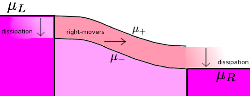
Figure 2: (color online) Illustration of the Landauer-type boundary condition (8). The right (left) moving eigenmodes are in chemical equilibrium with the electrons at the left (right) lead.

The measured voltage is then the difference in the electro-chemical potential between the leads:

$$V=\varphi_{L}+\mu_{L}/e-\varphi_{R}-\mu_{R}/e,$$ (9)

where we have written $\varphi(x_{L,R})\equiv\varphi_{L,R}$. This quantity will be finite whenever a finite current is flowing. Thus, since no dissipation is assumed to occur within the wire, it is only through a proper description of the contact between the wire and the leads, where dissipation occurs, that the current-voltage relation can be determined unambiguously glazman-88jetp238 ; landauer87zpb ; imry86 . In order to proceed, we now need to determine $\mu^{+}(x)$ and $\mu^{-}(x)$. To this end, we decouple the equations of motions, i.e., (3) and (4). (In this part of the calculation, the electric potential is not important, so we will set it to zero.) We define safi-95prb17040 :

$$\rho_{\pm}(x)=\frac{1}{2}(\rho(x)\pm j(x)/v(x)),$$ (10)

which by (3) and (4) yields

$$\partial_{t}\rho_{\pm} = \mp\partial_{x}(v(x)\rho_{\pm}(x))$$ (11)

$$\pm\frac{1}{2}(\partial_{x}K(x))\frac{v(x)}{K(x)}(\rho_{+}(x)+\rho_{-}(x)).$$

We see that a complete decoupling is achieved only in parts of the wire where $K(x)\approx\text{const}$ holds. In this case, we have a complete decoupling between the quantities $\rho_{-}$ and $\rho_{+}$, which can be interpreted as rightmoving and leftmoving densities, respectively. However, whenever we have a non-constant $K(x)$, rightmovers will be scattered into leftmovers at some finite rate and vice versa. As explained above, we assume that $K(x)$ is approximately constant (and equal to $1$) at the ends of the wire, as a consequence of the proximity to the metallic leads. It is only in this case that we have a truly “ballistic” situation of independent rightmoving and leftmoving populations with separate chemical potentials, and that the boundary conditions (8) at the contacts are well defined in an obvious way.

IV DC conductance

Independent of the spatial dependence of $K(x)$, however, we can write the Hamiltonian (1) (or rather, the charge part thereof) as a sum of a $\rho_{+}$–part and a $\rho_{-}$–part:

$$H=\frac{\pi}{2}\int dx\,\frac{v(x)}{K(x)}\left(\rho_{+}(x)^{2}+\rho_{-}(x)^{2}\right).$$ (12)

Note that with the definition (10), Eq. (12) holds even where $K(x)$ is not constant, i.e. in regions of the wire where the decoupling into left- and right-movers does not hold at the equation of motion level. Eq. (12) naturally leads to the definition of a local rightmoving and leftmoving chemical potential:

$$\mu^{\pm}(x)=\frac{\delta H}{\delta\rho_{\pm}(x)}=\pi\frac{v(x)}{K(x)}\,\rho_{\pm}(x).$$ (13)

As anticipated, we have $\mu(x)=\frac{1}{2}(\mu^{+}(x)+\mu^{-}(x))$. We are now in a position to address the main question: Are the boundary conditions (8) sufficient to uniquely specify the voltage–current relationship? We start with (7) in the following form:

$$\mu(x_{L})+e\varphi_{L}=\mu(x_{R})+e\varphi_{R}.$$ (14)

Expressing $\mu$ through $\mu^{+}$ and $\mu^{-}$, we can bring this equation into the form:

$$\begin{split}&\mu^{+}(x_{L})/e+\varphi_{L}-\mu^{-}(x_{R})/e-\varphi_{R}=\\ &\frac{1}{2}\left(\mu^{+}(x_{L})-\mu^{-}(x_{L})+\mu^{+}(x_{R})-\mu^{-}(x_{R})\right)/e.\end{split}$$ (15)

From (8) and (9), the left hand side is just the voltage $V$ across the wire. As for the right hand side, we note that using Eqs. (10) and (13), we have $j(x)=\pi^{-1}K(x)(\mu^{+}(x)-\mu^{-}(x))$. Given that $j(x)\equiv I/e$ is constant in a steady situation, where $I$ is the electric current, the last equation becomes

$$V=\frac{\pi}{2e^{2}}(\frac{1}{K_{L}}+\frac{1}{K_{R}})\,I.$$ (16)

Here, $K_{L,R}$ are the values of $K(x)$ at the contacts. From different approaches, this expression has been obtained before in the literature. As such, our framework also allows to describe generalized reservoirs in (16) that are either of Fermi liquid or Luttinger liquid type (encoded in $K_{L}$ and $K_{R}$), given that the proximity boundary conditions are still justified. If we put back our original assumption Eq. (2) that $K(x)$ approaches its “Fermi liquid” value $1$ near the leads, i.e. $K_{L}=K_{R}=1$, we obtain the conductance $G=I/V=\frac{e^{2}}{\pi}$. Or, putting back $\hbar$, which we had thus far set equal to $1$:

$$G=\frac{2e^{2}}{2\pi\hbar}=2\frac{e^{2}}{h}.$$ (17)

Hence, the conductance is quantized independent of the interactions in the bulk of the wire, but depending on the validity of the boundary conditions (2) and (8) only.

An alternative derivation of this result using equations of motion has been given by Safi in Ref. safi97, , where the equations of motion are argued to determine a particle transmission coefficient $T$. In our case, the use of the boundary conditions (8) allows us to completely avoid the concept of single particle transmission. The same boundary conditions are also used later by Safi in Ref. safi99ejp451, . Unlike there, however, a complete decoupling of the dynamics of left- and rightmoving degrees of freedom is not possible in the present context, as evidenced by Eq. (11). Even earlier, Eq. (8) has been employed in Ref. oreg-96prb14265, in an argument that is identical to ours in the non-interacting case, but not otherwise. We will further comment on the relation of our work to Ref. oreg-96prb14265, below.

V AC conductance

Aspects of the dynamical response of Luttinger liquids and one-dimensional conductors in general have been frequently addressed before pretre . In the time-reversal invariant case, the AC-conductance for special interaction profiles has been studied by Safi and Schulzsafi-95prb17040 , and Safisafi97annal . Quantum Hall edges have been considered by Oreg and Finkel’steinyuval95 . Here we derive a general result for the time-reversal invariant case with arbitrary interaction profile. To this end, we will restrict ourselves to frequencies much less than $v/L$, where $v$ is the typical mode velocity. Using Eq. 6, in the presence of a time-dependent current, Eq. 14 is modified according to

$$\mu(x_{L})+e\varphi(x_{L})-\mu(x_{R})+e\varphi(x_{R})=\int_{-L/2}^{L/2}dx\,\partial j_{t}(x)\Lambda(x).$$ (18)

We assume the general mode expansion of the particle current to be of the form

$$j_{\omega}(x,t)=e^{-i\omega t}\sum_{k}j_{k}(\omega)e^{ikx},$$ (19)

where the mode coefficients $j_{k}(\omega)$ are assumed to be analytic functions of $\omega$. We know that in the DC limit, the current does not depend on $x$, i.e. $j_{k}(\omega)|_{\omega=0}\propto\delta_{k,0}$. This implies

$$j_{k}(\omega)=\mathcal{O}(\omega)\;\;\;\forall k\neq 0.$$ (20)

With these assumptions, we plug Eq. 19 into Eq. 18. We keep only the leading term in $\omega$, which only depends on $j_{k=0}(\omega)\equiv\bar{I}(\omega)/e$. With this, Eq. 18 yields an AC generalization of Eq.15:

$$\mu^{+}(x_{L})/e+\varphi_{L}-\mu^{-}(x_{R})/e-\varphi_{R}=-\frac{i\omega\pi\tau}{e^{2}}\bar{I}(\omega)e^{-i\omega t}$$

$$+\frac{1}{2e}\left(\mu^{+}(x_{L})-\mu^{-}(x_{L})+\mu^{+}(x_{R})-\mu^{-}(x_{R})\right),$$

where the parameter $\tau$ is given by

$$\tau=1/\pi\int_{-L/2}^{L/2}dx\Lambda(x),$$ (22)

with $\Lambda(x)$ as defined in (6). As before, the expression in the second line of Eq. (V) equals $(I_{R}+I_{L})\pi/2e^{2}$, where $I_{R}$ and $I_{L}$ denote the current in the left and right lead, respectively. Due to possible capacitive effects, we no longer assume $I_{R}=I_{L}$, but define $I(\omega)e^{-i\omega t}=(I_{R}(t)+I_{L}(t))/2$. From Eq. 20, it is clear that $\bar{I}(\omega)=I(\omega)+\mathcal{O}(\omega)$. Identifying again the LHS of Eq. (V) with $Ve^{-i\omega t}$, we finally find the following relation between $V$ and $I(\omega)$:

$$I(\omega)=V\frac{2e^{2}/h}{1-i\omega\tau}.$$ (23)

Strictly speaking, this relation is obtained only for the small $\omega$ limit. However, we prefer to keep it in the above form which is manifestly Drude’s law. An interesting property of this low frequency limit is that while non-universal corrections enter through the parameter $\tau$ given by Eq. (22), details such as the functional relation between the potential $\varphi(x)$ and the charge distribution on the wire do not enter. These details would be sensitive to aspects such as wire geometry, and could in principle affect higher order corrections. In contrast, $\tau$ is solely determined by the value of the Luttinger parameter within the wire. This would allow one to compare $\tau$ as determined by AC measurements to other means of extracting the Luttinger parameter.

VI Discussion

The derivation given here emphasizes that two ingredients are sufficient to observe the quantized conductance in interacting quantum wires. The “proximity” boundary condition Eq. (2) implies that the interactions in the quantum wire become gradually weaker as the Fermi liquid leads are approached, as originally emphasized in Refs. maslov-95prb5539, ; safi-95prb17040, . The “chemical” boundary conditions Eq. (8) imply that the rightmoving (leftmoving) electrons of the wire are in chemical equilibrium with electrons of the left (right) reflectionless contact. We note that if we relax condition (2) by allowing $K(x_{R})$ and $K(x_{L})$ to take on a common value $K\neq 1$ (and in particular if $K(x)=K=\text{const.}$), Eq. (16) yields the Kane-Fisher result kane-92prl1220 , according to which the conductance is renormalized via $G=2Ke^{2}/h$.

We note that the physical assumptions leading to the quantized DC conductance in our framework are compatible with those made by a number of other workers (e.g. Refs. safi-95prb17040, ; maslov-95prb5539, ; alekseev-98prl3503, ; lehur-08ap3037, ; lebedev-05prb075416, ). On the other hand, alternative views are also found in the literature. Notably, in Ref. oreg-96prb14265, , a quantized conductance of $G=e^{2}/h$ is found for interacting spinless 1D fermions, within an approach which does not directly involve boundary conditions of the type Eq. (2). Instead, following Ref. kawabata95jpsj30, , it is argued that the quantized value is always obtained when electron-electron interaction effects are self-consistently included into the definition of the total electric field. We will now clarify the relation of this approach to ours (see Ref. safi97, for a different discussion). We first observe that such interaction effects also enter the definition of our total voltage, Eq. (9). Here, the Hartree mean field part of the interactions is included in the potential $\varphi(x)$, while correlation effects are included in the definition of the right- and left-moving local chemical potential, Eq. (13). In addition, however, these chemical potentials do not depend on interactions alone, but equally depend on the kinetic part of the Hamiltonian, through their dependence on the local density. This is in accordance with the general notion that in gapless 1D systems, kinetic energy and interactions should be treated on equal footings, as is manifest by their form in the Luttinger Hamiltonian.

The difference between the approach discussed here and those emphasizing self-consistent fields over boundary conditions of the form Eq. (2) can be understood as follows. It is useful to discuss both spinless and spinful fermions for a homogeneous wire with $K(x)=K=const$. In the spinful case, our result reduces to that of Kane and Fisher, $G=2Ke^{2}/h$. This value coincides with that for non-interacting spinless fermions, $e^{2}/h$, if $K$ equals $1/2$. This again is entirely consistent with the well-known fact that for $K=1/2$, the charge part of Eq. (1) is identical to the Hamiltonian of non-interacting spinless fermions. (This remains true in the presence of an electromagnetic field.) Thus, in the absence of boundary conditions, at least naively nothing should distinguish the two cases. If, on the other hand, one concludes that the conductance is unrenormalized, even in the homogeneous wire case with unspecified boundary conditions, one would obtain $G=2e^{2}/h$ for spinful fermions even at $K=1/2$, whereas $G=e^{2}/h$ for non-interacting spinless fermions. This may seem somewhat at odds with the fact that the charge part of the Hamiltonian is exactly the same in both cases. The only difference in these two cases is the decomposition of the Hamiltonian into distinct kinetic and interacting parts. In the present approach, where these parts are treated on equal footing throughout, a difference in conductance may only arise through different boundary conditions. Indeed, with our conventions, these boundary conditions must read $K_{L}=K_{R}=1/2$ if the system, including leads, consists of spinless fermions. On the other hand, a major difference between our treatment and that in Refs. kawabata95jpsj30, ; oreg-96prb14265, lies in the definition of the measured voltage. While we include a chemical potential drop between the leads, which is related to a chemical potential difference between rightmovers and leftmovers by Eq. (8), in Refs. kawabata95jpsj30, ; oreg-96prb14265, the voltage is just the integral over the total electric field. This may be a more natural definition in a truly homogeneous wire without boundaries. The chemical potential difference included into our voltage is always finite (for the homogeneous wire) in the presence of a finite current. This explains why in the homogeneous wire case, our result for the conductance (renormalized) will in general differ from that of Refs. kawabata95jpsj30, ; oreg-96prb14265, (unrenormalized). We do believe that in most experiments conducted so far, where a voltage is measured between two leads and Landauers basic ideas apply, the voltage definition used here is the appropriate one, and the observed conductance is thus entirely determined by boundary conditions of the kind used here. We note, however, that experimental setups have been proposed maslov04 which circumvent the application of leads altogether by measuring alternating currents induced in the wire by a resonator. The approach of Refs. kawabata95jpsj30, ; oreg-96prb14265, may indeed be better suited to describe this case. Such experiments would hence be very useful to distinguish the picture developed here and elsewhere from others.

We finally remark that although we did not develop a detailed scenario for possible deviations from the quantized value of the conductance matveev04prb245319 ; danneau-08prl016403 ; thomas-96prl135 , we are confident that the explanation for such deviations may be addressed similarly if proper boundary conditions describing these cases are identified. One interesting possibility is that a spin gap exists in the entire wire including the contacts. In this case one may conjecture that the spinless case effectively applies with an effective charge $e^{\ast}=2e$ (Ref. KYpriv, , c.f. also Ref. seidel-05prb045113, ). However, the interactions can then not be considered weak at the boundary, and we defer a detailed analysis to further studies. Moreover, we conjecture that our treatment of the AC conductance largely carries over to these cases. Since deviations from the $\omega\rightarrow 0$ limit are expressible solely through bulk properties of the wire, the natural modification of Eq. (23) would be to simply replace the numerator by the respective non-universal value of the DC conductance. The Drude-type expression (23) we find in the AC case may also suggest that this expression could be obtained in an ”RPA-like” approximation. If so, this may suggest that the validity of this expression can be extended beyond the $\omega\ll v/L$ regime. We note, however, that $v/L$ typically well exceeds the gigahertz range under relevant conditions, and so the restriction $\omega\ll v/L$ should not pose a stringent limitation for current experiments.

VII Conclusion

In this article we addressed the fundamental nature of quantized conductance in one-dimensional quantum wires. Working in a framework based on the analysis of the equations of motion of an inhomogeneous interacting Luttinger liquid, we argued for the significance of two types of boundary conditions as the underlying cause for a quantized conductance. The formalism presented here simplifies some earlier treatments without loss of essential physics, and should serve as a useful starting point also when discussing possible deviations from the ideal quantized conductance. We have further studied AC deviations from the universal conductance, and found that these are expressible through general Luttinger parameters in a simple manner in the low frequency limit.

- (1) R. Landauer, IBM J. Res. Dev. 1, 233 (1957).
- (2) R. Landauer, Philos. Mag. 21, 863 (1970).
- (3) R. Landauer, Z. Phys. B 68, (1987).
- (4) M. Büttiker, Phys. Rev. Lett. 57, 1761 (1986).
- (5) B. J. van Wees, H. van Houten, C. W. J. Beenakker, J. G. Williamson, L. P. Kouwenhoven, D. van der Marel, and C. T. Foxon, Phys. Rev. Lett. 60, 848 (1988).
- (6) D. A. Wharam, T. J. Thornton, R. Newbury, M. Pepper, H. Ahmed, J. E. F. Frost, D. G. Hasko, D. C. Peacock, D. A. Ritchie, and G. A. Jones, J. Phys. C 21, L209 (1988).
- (7) W. Apel and T. M. Rice, Phys. Rev. B 26, 7063 (1982).
- (8) C. L. Kane and M. P. A. Fisher, Phys. Rev. Lett. 68, 1220 (1992).
- (9) M. Ogata and H. Fukuyama, Phys. Rev. Lett. 73, 468 (1994).
- (10) A. Kawabata, J. Phys. Soc. Jp. 65, 30 (1995).
- (11) I. Safi and H. J. Schulz, Phys. Rev. B 52, R17040 (1995).
- (12) I. Safi, Phys. Rev. B 55, R7331 (1997).
- (13) V. V. Ponomarenko, Phys. Rev. B 52, R8666 (1995).
- (14) D. L. Maslov and M. Stone, Phys. Rev. B 52, R5539 (1995).
- (15) A. Y. Alekseev, V. V. Cheianov, and J. Fröhlich, Phys. Rev. Lett. 81, 3503 (1998).
- (16) V. V. Ponomarenko and N. Nagaosa, Phys. Rev. B 60, 16865 (1999).
- (17) I. Safi, Eur. Phys. J. B 12, 451 (1999).
- (18) K.-I. Imura, K.-V. Pham, P. Lederer, and F. Piéchon, Phys. Rev. B 66, 035313 (2002).
- (19) K.-V. Pham, M. Gabay, and P. Lederer, Phys. Rev. B 61, 16397 (2000).
- (20) B. Trauzettel, I. Safi, F. Dolcini, and H. Grabert, Phys. Rev. Lett. 92, 226405 (2004).
- (21) R. Danneau, O. Klochan, W. R. Clarke, L. H. Ho, A. P. Micolich, M. Y. Simmons, A. R. Hamilton, M. Pepper, and D. A. Ritchie, Phys. Rev. Lett. 100, 016403 (2008).
- (22) K. J. Thomas, J. T. Nicholls, M. Y. Simmons, M. Pepper, D. R. Mace, and D. A. Ritchie, Phys. Rev. Lett. 77, 135 (1996).
- (23) A. Yacoby, H. L. Stormer, N. S. Wingreen, L. N. Pfeiffer, K. W. Baldwin, and K. W. West, Phys. Rev. Lett. 77, 4612 (1996).
- (24) K. J. Thomas, J. T. Nicholls, M. Pepper, W. R. Tribe, M. Y. Simmons, and D. A. Ritchie, Phys. Rev. B 61, R13365 (2000).
- (25) A. Kristensen, H. Bruus, A. E. Hansen, J. B. Jensen, P. E. Lindelof, C. J. Marckmann, J. Nygård, C. B. Sørensen, F. Beuscher, A. Forchel, and M. Michel, Phys. Rev. B 62, 10950 (2000).
- (26) D. J. Reilly, T. M. Buehler, J. L. O’Brien, A. R. Hamilton, A. S. Dzurak, R. G. Clark, B. E. Kane, L. N. Pfeiffer, and K. W. West, Phys. Rev. Lett. 89, 246801 (2002).
- (27) M. J. Biercuk, N. Mason, J. Martin, A. Yacoby, and C. M. Marcus, Phys. Rev. Lett. 94, 026801 (2005).
- (28) S. M. Cronenwett, H. J. Lynch, D. Goldhaber-Gordon, L. P. Kouwenhoven, C. M. Marcus, K. Hirose, N. S. Wingreen, and V. Umansky, Phys. Rev. Lett. 88, 226805 (2002).
- (29) Y. Meir, K. Hirose, and N. S. Wingreen, Phys. Rev. Lett. 89, 196802 (2002).
- (30) K. A. Matveev, Phys. Rev. B 70, 245319 (2004).
- (31) O. P. Sushkov, Phys. Rev. B 64, 155319 (2001).
- (32) K. Janzen, V. Meden, and K. Schönhammer, Phys. Rev. B 74, 085301 (2006).
- (33) Y.-F. Chen, T. Dirks, G. Al-Zoubi, N. O. Birge, and N. Mason, Phys. Rev. Lett. 102, 036804 (2009).
- (34) O. M. Auslaender, A. Yacoby, R. de Picciotto, K. W. Baldwin, L. N. Pfeiffer, and K. W. West, Science 295, 825 (2002).
- (35) F. D. M. Haldane, Phys. Rev. Lett. 47, 1840 (1981).
- (36) A. V. Lebedev, A. Crépieux, and T. Martin, Phys. Rev. B 71, 075416 (2005).
- (37) A. Seidel and D.-H. Lee, Phys. Rev. B 71, 045113 (2005).
- (38) D. Maslov, in LXXXI Les Houches Summer School (Elsevier, Amsterdam, 2005), Chap. Nanophysics: Coherence and Transport.
- (39) K. Le Hur, B. I. Halperin, and A. Yacoby, Ann. Phys. 323, 3037 (2008).
- (40) L. I. Glazman, G. B. Lesovik, Khmel’nitskii, and R. I. Shekhter, JETP Lett. 48, 238 (1988).
- (41) Y. Imry, Directions in Condensed Matter (World Scientific, Singapore, 1986).
- (42) Y. Oreg and A. M. Finkel’stein, Phys. Rev. B 54, R14265 (1996).
- (43) M. Büttiker, A. Prêtre, and H. Thomas, Phys. Rev. Lett. 70, 4114 (1993).
- (44) I. Safi, Ann. Phys. Fr. 22, 463 (1997).
- (45) Y. Oreg and A. M. Finkel’stein, Phys. Rev. Lett. 74, 3668 (1995).
- (46) K. Yang, private communication.