Measures of Variability for Bayesian Network Graphical Structures

Abstract

The structure of a Bayesian network includes a great deal of information about the probability distribution of the data, which is uniquely identified given some general distributional assumptions. Therefore it’s important to study its variability, which can be used to compare the performance of different learning algorithms and to measure the strength of any arbitrary subset of arcs.

In this paper we will introduce some descriptive statistics and the corresponding parametric and Monte Carlo tests on the undirected graph underlying the structure of a Bayesian network, modeled as a multivariate Bernoulli random variable. A simple numeric example and the comparison of the performance of some structure learning algorithm on small samples will then illustrate their use.

1 Introduction

In recent years Bayesian networks have been successfully applied in several different disciplines, including medicine, biology and epidemiology (see for example Friedman et al. [1] and Holmes and Jain [2]). This has been made possible by the rapid evolution of structure learning algorithms, from constraint-based ones (such as PC [3], Grow-Shrink [4], IAMB [5] and its variants [6]) to score-based (such as TABU search [7], Greedy Equivalent Search [8] and genetic algorithms [9]) and hybrid ones (such as Max-Min Hill Climbing [10]).

The main goal in the development of these algorithms has been the reduction of the number of either independence tests or score comparisons needed to learn the structure of the Bayesian network. Their correctness has been proved assuming either very large sample sizes in relation to the number of variables (in the case of Greed Equivalent Search) or the absence of both false positives and false negatives (in the case of Grow-Shrink and IAMB). In most cases the characteristics of the learned networks were studied using a small number of reference data sets [11] as benchmarks, and differences from the true structure measured with purely descriptive measures such as Hamming distance [12].

This approach to model evaluation is not possible for real world data sets, as the true structure of their probability distribution is not known. An alternative is provided by the use of either parametric or nonparametric bootstrap [13]. By applying a learning algorithm to a sufficiently large number of bootstrap samples it is possible to obtain the empirical probability of any feature of the resulting network [14], such as the structure of the Markov Blanket of a particular node. The fundamental limit in the interpretation of the results is that the “reasonable” level of confidence for thresholding depends on the data.

In this paper we propose a modified bootstrap-based approach for the inference on the structure of a Bayesian network. The undirected graph underlying the network structure is modeled as a multivariate Bernoulli random variable in which each component is associated with an arc. This assumption allows the derivation of both exact and asymptotic measures of the variability of the network structure or any of its parts.

2 Bayesian networks and bootstrap

Bayesian networks are graphical models where nodes represent random variables (the two terms are used interchangeably in this article) and arcs represent probabilistic dependencies between them [15].

The graphical structure $\mathcal{G}=(\mathbf{V},A)$ of a Bayesian network is a directed acyclic graph (DAG) which defines a factorization of the joint probability distribution of $\mathbf{V}=\{X_{1},X_{2},\ldots,X_{v}\}$, often called the global probability distribution, into a set of local probability distributions, one for each variable. The form of the factorization is given by the Markov property of Bayesian networks, which states that every random variable $X_{i}$ directly depends only on its parents $\Pi_{X_{i}}$.

Therefore it is important to define confidence and variability measures for specific features in the network structure, such as the presence of specific configurations of arcs. In particular a measure of variability for the network structure as a whole has many applications both as an indicator of goodness of fit for a particular Bayesian network and as a criterion to evaluate the performance of a learning algorithm.

Confidence measures have been developed by Friedman et al. [14] using bootstrap simulation, and later modified by Imoto et al. [16] to estimate the marginal confidence in the presence of an arc (called edge intensity, and also known as arc strength) and its direction. This approach can be summarized as follows:

1. For $b=1,2,\ldots,m$

   1. re-sample a new data set $\mathbf{D^{*}_{b}}$ from the original data $\mathbf{D}$ using either parametric or nonparametric bootstrap.

   2. learn a Bayesian network $\mathcal{G}_{b}$ from $\mathbf{D^{*}_{b}}$.

2. Estimate the confidence in each feature $f$ of interest as $\hat{\mathsf{P}}(f)=(1/m)\sum_{b=1}^{m}f(\mathcal{G}_{b})$.

However, the empirical probabilities $\hat{\mathsf{P}}(f)$ are difficult to evaluate, because the distribution of $\mathcal{G}$ in the space of DAGs is unknown and because the confidence threshold value depends on the data.

3 The multivariate Bernoulli distribution

Let $B_{1},B_{2},\ldots,B_{k}$, $k\in\mathbb{N}$ be Bernoulli random variables with marginal probability of success $p_{1},p_{2},\ldots,p_{k}$, that is $B_{i}\sim Ber(p_{i})$, $i=1,\ldots,k$. Then the distribution of the random vector $\mathbf{B}=[B_{1},B_{2},\ldots,B_{k}]^{T}$ over the joint probability space of $B_{1},B_{2},\ldots,B_{k}$ is a multivariate Bernoulli random variable [17], denoted as $Ber_{k}(\mathbf{p})$. Its probability function is uniquely identified by the parameter collection $\mathbf{p}=\left\{p_{I}:I\subseteq\{1,\ldots,k\},I\neq\varnothing\right\}$, which represents the dependence structure among the marginal distributions in terms of simultaneous successes for every non-empty subset $I$ of elements of $\mathbf{B}$.

However, several useful results depend only on the first and second order moments of $\mathbf{B}$

$$\mathsf{E}(B_{i}) =p_{i}$$ (1)

$$\mathsf{VAR}(B_{i}) =\mathsf{E}(B_{i}^{2})-\mathsf{E}(B_{i})^{2}=p_{i}-p_{i}^{2}$$ (2)

$$\mathsf{COV}(B_{i},B_{j}) =\mathsf{E}(B_{i}B_{j})-\mathsf{E}(B_{i})\mathsf{E}(B_{j})=p_{ij}-p_{i}p_{j}$$ (3)

and the reduced parameter collection $\mathbf{\tilde{p}}=\left\{p_{ij}:i,j=1,\ldots,k\right\}$, which can be used as an approximation of $\mathbf{p}$ in the generation random multivariate Bernoulli vectors in Krummenauer [18].

3.1 Uncorrelation and independence

We will first consider a simple result that links covariance and independence of two univariate Bernoulli variables.

Theorem 1.

Let $B_{i}$ and $B_{j}$ be two Bernoulli random variables. Then $B_{i}$ and $B_{j}$ are independent if and only if they are uncorrelated.

Proof.

If $B_{i}$ and $B_{j}$ are independent, then by definition $\mathsf{COV}(B_{i},B_{j})=0$. If on the other hand we have that $\mathsf{COV}(B_{i},B_{j})=0$, then $p_{ij}=p_{i}p_{j}$ which completes the proof. ∎

This theorem can be extended to multivariate Bernoulli random variables as follows.

Theorem 2.

Let $\mathbf{B}=[B_{1},B_{2},\ldots,B_{k}]^{T}$ and $\mathbf{C}=[C_{1},C_{2},\ldots,C_{l}]^{T}$, $k,l\in\mathbb{N}$ be two multivariate Bernoulli random variables. Then $\mathbf{B}$ and $\mathbf{C}$ are independent if and only if $\mathsf{COV}(\mathbf{B},\mathbf{C})=\mathbf{O}$, where $\mathbf{O}$ is the zero matrix.

Proof.

If $\mathbf{B}$ is independent from $\mathbf{C}$, then by definition every pair $(B_{i},C_{j})$, $i=1,\ldots,k$, $j=1,\ldots,l$ is independent. Therefore $\mathsf{COV}(\mathbf{B},\mathbf{C})=[c_{ij}]=\mathbf{O}$.

If conversely $\mathsf{COV}(\mathbf{B},\mathbf{C})=\mathbf{O}$, every pair $(B_{i},C_{j})$ is independent as $c_{ij}=0$ implies $p_{ij}=p_{i}p_{j}$. This in turn implies the independence of the random vectors $\mathbf{B}$ and $\mathbf{C}$, as their sigma-algebras $\sigma(\mathbf{B})=\sigma(B_{1})\times\ldots\times\sigma(B_{k})$ and $\sigma(\mathbf{C})=\sigma(C_{1})\times\ldots\times\sigma(C_{l})$ are functions of the sigma-algebras induced by the two sets of independent random variables $B_{1},B_{2},\ldots,B_{k}$ and $C_{1},C_{2},\ldots,C_{l}$. ∎

The correspondence between uncorrelation and independence is identical to the analogous property of the multivariate Gaussian distribution [19], and is closely related to the strong normality defined for orthogonal second order random variables in Loève [20]. It can also be applied to disjoint subsets of components of a single multivariate Bernoulli variable, which are also distributed as multivariate Bernoulli random variables.

Theorem 3.

Let $\mathbf{B}=[B_{1},B_{2},\ldots,B_{k}]^{T}$ be a multivariate Bernoulli random variable; then every random vector $\mathbf{B^{*}}=[B_{i_{1}},B_{i_{2}},\ldots,B_{i_{l}}]^{T}$, $\left\{i_{1},i_{2},\ldots,i_{l}\right\}\subseteq\left\{1,2,\ldots,k\right\}$ is a multivariate Bernoulli random variable.

Proof.

The marginal components of $\mathbf{B^{*}}$ are Bernoulli random variables, because $\mathbf{B}$ is multivariate Bernoulli. The new dependency structure is defined as $\mathbf{p^{*}}=\left\{p_{I^{*}}:I^{*}\subseteq\{i_{1},\ldots,i_{l}\},I^{*}\neq\varnothing\right\}$, and uniquely identifies the probability distribution of $\mathbf{B^{*}}$. ∎

3.2 Properties of the covariance matrix

The covariance matrix $\Sigma=[\sigma_{ij}]$, $i,j=1,\ldots,k$ associated with a multivariate Bernoulli random vector has several interesting numerical properties. Due to the form of the central second order moments defined in formulas 2 and 3, the diagonal elements $\sigma_{ii}$ are bounded in the interval $[0,1/4]$. The maximum is attained for $p_{i}=1/2$, and the minimum for both $p_{i}=0$ and $p_{i}=1$. For the Cauchy-Schwarz theorem [19] then $|\sigma_{ij}|\in\left[0,1/4\right]$.

The eigenvalues $\lambda_{1},\lambda_{2},\ldots,\lambda_{k}$ of $\Sigma$ are similarly bounded, as shown in the following theorem.

Theorem 4.

Let $\mathbf{B}=[B_{1},B_{2},\ldots,B_{k}]^{T}$ be a multivariate Bernoulli random variable, and let $\Sigma=[\sigma_{ij}]$, $i,j=1,\ldots,k$ be its covariance matrix. Let $\lambda_{i}$, $i=1,\ldots,k$ be the eigenvalues of $\Sigma$. Then $0\leqslant\sum_{i=1}^{k}\lambda_{i}\leqslant k/4$ and $0\leqslant\lambda_{i}\leqslant k/4$.

Proof.

Since $\Sigma$ is a real, symmetric, non-negative definite matrix, the eigenvalues $\lambda_{i}$ are non-negative real numbers [21]; this proves the lower bound in both inequalities.

The upper bound in the first inequality holds because

$$\sum_{i=1}^{k}\lambda_{i}=\sum_{i=1}^{k}\sigma_{ii}\leqslant\max_{\left\{\sigma_{ii}\right\}}\sum_{i=1}^{k}\sigma_{ii}=\sum_{i=1}^{k}\max\sigma_{ii}=\frac{k}{4},$$ (4)

and this in turn implies $\lambda_{i}\leqslant\sum_{i=1}^{k}\lambda_{i}\leqslant k/4$, which completes the proof. ∎

These bounds define a convex set in $\mathbb{R}^{k}$, defined by the family

$$\mathcal{D}=\left\{\Delta^{k-1}(c):c\in\left[0,\frac{k}{4}\right]\right\}$$ (5)

where $\Delta^{k-1}(c)$ is the non-standard $k-1$ simplex

$$\Delta^{k-1}(c)=\left\{(\lambda_{1},\ldots,\lambda_{k})\in\mathbb{R}^{k}:\sum_{i=1}^{k}\lambda_{i}=c,\lambda_{i}\geqslant 0\right\}.$$ (6)

3.3 Sequences of multivariate Bernoulli variables

Consider now a sequence of independent and identically distributed multivariate Bernoulli variables $\mathbf{B_{1}},\mathbf{B_{2}},\ldots,\mathbf{B_{m}}\sim Ber_{k}(\mathbf{p})$. The sum

$$\mathbf{S}_{m}=\sum_{i=1}^{m}\mathbf{B}_{i}\sim Bi_{k}(m,\mathbf{p})$$ (7)

is distributed as a multivariate Binomial random variable [17], thus preserving one of the fundamental properties of the univariate Bernoulli distribution. A similar result holds for the law of small numbers, whose multivariate version states that a $k$-variate Binomial distribution $Bi_{k}(m,\mathbf{p})$ converges to a multivariate Poisson distribution $P_{k}(\mathbf{\Lambda})$:

$$\mathbf{S}_{m}\stackrel{{\scriptstyle d}}{{\to}}P_{k}(\mathbf{\Lambda}) m\mathbf{p}\to\mathbf{\Lambda}.$$ as (8)

Both these distributions’ probability functions, while tractable, are not very useful as a basis for closed-form inference procedures. An alternative is given by the asymptotic multivariate Gaussian distribution defined by the multivariate central limit theorem [19]:

$$\frac{\mathbf{S}_{m}-m\mathsf{E}(\mathbf{B}_{1})}{\sqrt{m}}\stackrel{{\scriptstyle d}}{{\to}}N_{k}(\mathbf{0},\Sigma).$$ (9)

The limiting distribution is guaranteed to exist for all possible values of $\mathbf{p}$, as the first two moments are bounded and therefore are always finite.

4 Inference on the network structure

Let $\mathcal{U}=(\mathbf{V},E)$ be the undirected graph underlying a DAG $\mathcal{G}=(\mathbf{V},A)$, defined as its unique biorientation [22]. Each edge $e\in E$ of $\mathcal{U}$ corresponds to the directed arcs in $A$ with the same incident nodes, and has only two possible states (it’s either present in or absent from the graph).

Then each possible edge $e_{i}$, $i=1,\ldots,|\mathbf{V}|(|\mathbf{V}|-1)/2$ is naturally distributed as a Bernoulli random variable

$$E_{i}=\left\{\begin{aligned} e_{i}&\in E&&\text{with probability $p_{i}$}&\\ e_{i}&\not\in E&&\text{with probability $1-p_{i}$}&\end{aligned}\right.$$ (10)

and every set $W\subseteq\mathbf{V}\times\mathbf{V}$ (including $E$) is distributed as a multivariate Bernoulli random variable $\mathbf{W}$ and identified by the parameter collection $\mathbf{p}_{W}=\left\{p_{w}:w\subseteq W,w\neq\varnothing\right\}$. The elements of $\mathbf{p}_{W}$ can be estimated via parametric or nonparametric bootstrap as in Friedman et al. [14], because they are functions of the DAGs $\mathcal{G}_{b}$, $b=1,\ldots,m$ through the underlying undirected graphs $\mathcal{U}_{b}=(V,E_{b})$. The resulting empirical probabilities

$$\hat{p}_{w}=\frac{1}{m}\sum_{b=1}^{m}\mathbb{I}_{\left\{w\subseteq E_{b}\right\}}(\mathcal{U}_{b}),$$ (11)

in particular

$$\hat{p}_{i}=\frac{1}{m}\sum_{b=1}^{m}\mathbb{I}_{\left\{e_{i}\in E_{b}\right\}}(\mathcal{U}_{b}) \hat{p}_{ij}=\frac{1}{m}\sum_{b=1}^{m}\mathbb{I}_{\left\{e_{i}\in E_{b},e_{j}\in E_{b}\right\}}(\mathcal{U}_{b}),$$ and (12)

can be used to obtain several descriptive measures and test statistics for the variability of the structure of a Bayesian network.

4.1 Interpretation of bootstrapped networks

Considering the undirected graphs $\mathcal{U}_{1},\ldots,\mathcal{U}_{m}$ instead of the corresponding directed graphs $\mathcal{G}_{1},\ldots,\mathcal{G}_{m}$ greatly simplifies the interpretation of bootstrap’s results. In particular the variability of the graphical structure can be summarized in three cases according to the entropy [23] of the set of the bootstrapped networks:

• minimum entropy: all the networks learned from the bootstrap samples have the same structure, that is $E_{1}=E_{2}=\ldots=E_{m}=E$. This is the best possible outcome of the simulation, because there is no variability in the estimated network. In this case the first two moments of the multivariate Bernoulli distribution are equal to

  $$p_{i}=\left\{\begin{aligned} &1&&\text{if $e_{i}\in E$}\\ &0&&\text{otherwise}&\end{aligned}\right. \Sigma=\mathbf{O}.$$ and (13)

• intermediate entropy: several network structures are observed with different frequencies $m_{b}$, $\sum m_{b}=m$. The first two sample moments of the multivariate Bernoulli distribution are equal to

  $$\hat{p}_{i}=\frac{1}{m}\sum_{b\,:\,e_{i}\in E_{b}}m_{b} \hat{p}_{ij}=\frac{1}{m}\sum_{b\,:\,e_{i}\in E_{b},e_{j}\in E_{b}}m_{b}.$$ and (14)

• maximum entropy: all $2^{|\mathbf{V}|(|\mathbf{V}|-1)/2}$ possible network structures appear with the same frequency, that is

  $$\hat{\mathsf{P}}(\mathcal{U}_{i})=\frac{1}{2^{|\mathbf{V}|(|\mathbf{V}|-1)/2}} i=1,\ldots,2^{|\mathbf{V}|(|\mathbf{V}|-1)/2}.$$ (15)

  This is the worst possible outcome because edges vary independently of each other and each one is present in only half of the networks (proof provided in B):

  $$p_{i}=\frac{1}{2} \Sigma=\frac{1}{4}I_{k}.$$ and (16)

  This is also the only case in which all eigenvalues reach their maximum, that is $\lambda_{1}=\lambda_{2}=\ldots=\lambda_{k}=1/4$.

4.2 Descriptive statistics of network variability

Several functions have been proposed in literature as univariate measures of spread of a multivariate distribution, usually under the assumption of multivariate normality (see for example Muirhead [24] and Bilodeau and Brenner [25]). Three of them in particular can be used as descriptive statistics for the multivariate Bernoulli distribution:

• the generalized variance, $\mathsf{VAR}_{G}(\Sigma)=\det(\Sigma)$.

• the total variance, $\mathsf{VAR}_{T}(\Sigma)=\operatorname{tr}(\Sigma)$, also called total variation in Mardia et al. [26].

• the squared Frobenius matrix norm, $\mathsf{VAR}_{N}(\Sigma)=|||\Sigma-(k/4)I_{k}|||_{F}^{2}$.

Both generalized and total variance associate high values of the statistic to unstable network structures, and are bounded due to the properties of the covariance matrix $\Sigma$. For the total variance it’s easy to show that

$$0\leqslant\mathsf{VAR}_{T}(\Sigma)=\sum_{i=1}^{k}\sigma_{ii}\leqslant\frac{1}{4}k.$$ (17)

The generalized variance is similarly bounded due to Hadamard’s theorem on the determinant of a non-negative definite matrix [27]:

$$0\leqslant\mathsf{VAR}_{G}(\Sigma)\leqslant\prod_{i=1}^{k}\sigma_{ii}\leqslant\left(\frac{1}{4}\right)^{k}.$$ (18)

They reach the respective maxima in the maximum entropy case and are equal to zero only in the minimum entropy case. The generalized variance is also strictly convex (the maximum is reached only for $\Sigma=(1/4)I_{k}$), but it is equal to zero if $\Sigma$ is rank deficient. For this reason it’s convenient to reduce $\Sigma$ to a smaller, full rank matrix (let’s say $\Sigma^{*}$) and compute $\mathsf{VAR}_{G}(\Sigma^{*})$ instead of $\mathsf{VAR}_{G}(\Sigma)$.

The squared difference in Frobenius norm between $\Sigma$ and $k$ times the maximum entropy covariance matrix associates high values of the statistic to stable network structures. It can be rewritten in terms of the eigenvalues $\lambda_{1},\ldots,\lambda_{k}$ of $\Sigma$ as

$$\mathsf{VAR}_{N}(\Sigma)=\sum_{i=1}^{k}\left(\lambda_{i}-\frac{k}{4}\right)^{2}.$$ (19)

It has a unique maximum (in the minimum entropy case), which can be computed as the solution of the constrained minimization problem in $\boldsymbol{\lambda}=[\lambda_{1},\ldots,\lambda_{k}]^{T}$

$$\min_{\mathcal{D}}f(\boldsymbol{\lambda})=-\sum_{i=1}^{k}\left(\lambda_{i}-\frac{k}{4}\right)^{2} \lambda_{i}\geqslant 0,\sum_{i=1}^{k}\lambda_{i}\leqslant\frac{k}{4}$$ subject to (20)

using Lagrange multipliers [28]. It also has a single minimum in $\boldsymbol{\lambda}^{*}=[1/4,\ldots,1/4]$, which is the projection of $[k/4,\ldots,k/4]$ onto the set $\mathcal{D}$ and coincides with the maximum entropy case. The proof for these boundaries and the rationale behind the use of $(k/4)I_{k}$ instead of $(1/4)I_{k}$ are reported in A.

The corresponding normalized statistics are:

$$\overline{\mathsf{VAR}}_{T}(\Sigma) =\frac{\mathsf{VAR}_{T}(\Sigma)}{\max_{\Sigma}\mathsf{VAR}_{T}(\Sigma)}=\frac{4\mathsf{VAR}_{T}(\Sigma)}{k}$$ (21)

$$\overline{\mathsf{VAR}}_{G}(\Sigma) =\frac{\mathsf{VAR}_{G}(\Sigma)}{\max_{\Sigma}\mathsf{VAR}_{G}(\Sigma)}=4^{k}\mathsf{VAR}_{G}(\Sigma)$$ (22)

$$\overline{\mathsf{VAR}}_{N}(\Sigma) =\frac{\max_{\Sigma}\mathsf{VAR}_{N}(\Sigma)-\mathsf{VAR}_{N}(\Sigma)}{\max_{\Sigma}\mathsf{VAR}_{N}(\Sigma)-\min_{\Sigma}\mathsf{VAR}_{N}(\Sigma)}=\frac{k^{3}-16\mathsf{VAR}_{N}(\Sigma)}{k(2k-1)}.$$ (23)

All of them vary in the $[0,1]$ interval and associate high values of the statistic to networks whose structure display a high variability across the bootstrap samples. Equivalently we can define their complements $\overline{\overline{\mathsf{VAR}}}_{T}(\Sigma)$, $\overline{\overline{\mathsf{VAR}}}_{G}(\Sigma)$ and $\overline{\overline{\mathsf{VAR}}}_{N}(\Sigma)$, which associate high values of the statistic to networks with little variability and can be used as measures of distance from the maximum entropy case.

4.3 Asymptotic inference

The limiting distribution of the descriptive statistics defined above can be derived by replacing the covariance matrix $\Sigma$ with its unbiased estimator $\hat{\Sigma}$ and by considering the multivariate Gaussian distribution from equation 9. The hypothesis we are interested in is

$$H_{0}:\Sigma=\frac{1}{4}I_{k} H_{1}:\Sigma\neq\frac{1}{4}I_{k},$$ (24)

which relates the sample covariance matrix with the one from the maximum entropy case.

For the total variance we have that $t_{T}=4m\operatorname{tr}(\hat{\Sigma})\stackrel{{\scriptstyle.}}{{\sim}}\chi^{2}_{mk}$ [24], and since the maximum value of $\operatorname{tr}(\Sigma)$ is achieved in the maximum entropy case, the hypothesis in Equation 24 assumes the form

$$H_{0}:\operatorname{tr}(\Sigma)=\frac{k}{4} H_{1}:\operatorname{tr}(\Sigma)<\frac{k}{4}.$$ (25)

Then the observed significance value is $\hat{\alpha}_{T}=\mathsf{P}(t_{T}\leqslant t_{T}^{oss})$, and can be improved with the finite sample correction

$$\tilde{\alpha}_{T}=\mathsf{P}\left(t_{T}\leqslant t_{T}^{oss}\,|\,t_{T}\in[0,mk]\right)=\frac{\mathsf{P}(t_{T}\leqslant t_{T}^{oss})}{\mathsf{P}(t_{T}\leqslant mk)}$$ (26)

which accounts for the bounds on $\mathsf{VAR}_{T}(\Sigma)$ from inequality 17.

For the generalized variance there are several possible asymptotic and approximate distributions:

• the Gaussian distribution defined in Anderson [29]

  $$t_{G_{1}}=\sqrt{m}\left(\frac{\det(\hat{\Sigma})}{\det(\frac{1}{4}I_{k})}-1\right)\stackrel{{\scriptstyle.}}{{\sim}}N(0,2k).$$ (27)

• the Gamma distribution defined in Steyn [30]

  $$t_{G_{2}}=\frac{mk}{2}\sqrt[k]{\frac{\det(\hat{\Sigma})}{\det(\frac{1}{4}I_{k})}}\stackrel{{\scriptstyle.}}{{\sim}}Ga\left(\frac{k(m+1-k)}{2},1\right).$$ (28)

• the saddlepoint approximation defined in Butler et al. [31].

As before the hypothesis in Equation 24 assumes the form

$$H_{0}:\det(\Sigma)=\det\left(\frac{1}{4}I_{k}\right) H_{1}:\det(\Sigma)<\det\left(\frac{1}{4}I_{k}\right).$$ (29)

The observed significance values for the Gaussian and Gamma distributions are $\hat{\alpha}_{G_{1}}=\mathsf{P}(t_{G_{1}}\leqslant t_{G_{1}}^{oss})$ and $\hat{\alpha}_{G_{2}}=\mathsf{P}(t_{G_{2}}\leqslant t_{G_{2}}^{oss})$, and the respective finite sample corrections for the bounds on $\det(\Sigma)$ are

$$\tilde{\alpha}_{G_{1}} =\mathsf{P}\left(t_{G_{1}}\leqslant t_{G_{1}}^{oss}\,|\,t_{G_{1}}\in\left[-\sqrt{m},0\right]\right)=\frac{\mathsf{P}(t_{G_{1}}\leqslant t_{G_{1}}^{oss})-\mathsf{P}(t_{G_{1}}\leqslant-\sqrt{m})}{\mathsf{P}(t_{G_{1}}\leqslant 0)-\mathsf{P}(t_{G_{1}}\leqslant-\sqrt{m})}$$ (30)

$$\tilde{\alpha}_{G_{2}} =\mathsf{P}\left(t_{G_{2}}\leqslant t_{G_{2}}^{oss}\,|\,t_{G_{2}}\in\left[0,\frac{mk}{2}\right]\right)=\frac{\mathsf{P}(t_{G_{2}}\leqslant t_{G_{2}}^{oss})}{\mathsf{P}(t_{G_{2}}\leqslant\frac{mk}{2})}.$$ (31)

The test statistic associated with the squared Frobenius norm is the test for the equality of two covariance matrices defined in Nagao [32],

$$t_{N}=\frac{m}{2}\operatorname{tr}\left(\left[\hat{\Sigma}\left(\frac{1}{4}I_{k}\right)^{-1}-I_{k}\right]^{2}\right)=\frac{m}{2}\operatorname{tr}\left(\left[4\hat{\Sigma}-I_{k}\right]^{2}\right)\stackrel{{\scriptstyle.}}{{\sim}}\chi^{2}_{\frac{1}{2}k(k+1)},$$ (32)

because

$$\operatorname{tr}\left(\left[4\hat{\Sigma}-I_{k}\right]^{2}\right)=16\sum_{i=1}^{k}\left(\lambda_{i}-\frac{1}{4}\right)^{2}=16|||\hat{\Sigma}-\frac{1}{4}I_{k}|||_{F}^{2}$$ (33)

See A for an explanation of the use of $(1/4)I_{k}$ instead of $(k/4)I_{k}$. The significance value for $t_{N}$ is $\hat{\alpha}_{N}=\mathsf{P}(t_{N}\geqslant t_{N}^{oss})$ as the hypothesis in Equation 24 becomes

$$H_{0}:|||\Sigma-\frac{1}{4}I_{k}|||_{F}=0 H_{1}:|||\Sigma-\frac{1}{4}I_{k}|||_{F}>0.$$ (34)

Unlike the previous statistics, Nagao’s test displays a good convergence speed, to the point that the finite sample correction for the bounds on the squared Frobenius matrix norm

$$\tilde{\alpha}_{N}=\mathsf{P}\left(t_{N}\geqslant t_{N}^{oss}\,|\,t_{G_{1}}\in\left[0,t_{N}^{max}\right]\right)=\frac{\mathsf{P}(t_{N}\geqslant t_{N}^{oss})-\mathsf{P}(t_{N}>t_{N}^{max})}{\mathsf{P}(t_{N}\leqslant t_{N}^{max})}$$ (35)

is not appreciably better than the raw significance value (see Table 3 for a simple example).

4.4 Monte Carlo inference and parametric bootstrap

Another approach to compute the significance values associated with $\mathsf{VAR}_{T}(\Sigma)$, $\mathsf{VAR}_{G}(\Sigma)$ and $\mathsf{VAR}_{N}(\Sigma)$ is applying again parametric bootstrap.

The multivariate Bernoulli distribution $\mathbf{W}_{0}$ specified by the hypothesis in 24 has a diagonal covariance matrix, so its components $W_{0_{i}}$, $i=1,\ldots,k$ are uncorrelated. According to Theorem 1 they are also independent, so the joint distribution of $\mathbf{W}_{0}$ is completely specified by the marginal distributions $W_{0_{i}}\sim Ber(1/2)$. Therefore it’s possible (and indeed quite easy) to generate observations from the null distribution and use them to estimate the significance value of the normalized statistics $\overline{\overline{\mathsf{VAR}}}_{T}(\Sigma)$, $\overline{\overline{\mathsf{VAR}}}_{G}(\Sigma)$ and $\overline{\overline{\mathsf{VAR}}}_{N}(\Sigma)$ defined in section 4.2:

1. compute the value of test statistic $T$ on the original covariance matrix $\Sigma$.

2. For $r=1,2,\ldots,R$.

   1. generate $m$ sets of $k$ random samples from a $Ber(1/2)$ distribution.

   2. compute their covariance matrix $\Sigma^{*}_{r}$.

   3. compute $T^{*}_{r}$ from $\Sigma^{*}_{r}$

3. compute the Monte Carlo significance value as $\hat{\alpha}_{R}=(1/R)\sum_{r=1}^{R}\mathbb{I}_{\{x\geqslant T\}}(T^{*}_{r})$.

This approach has two important advantages over the parametric tests defined in section 4.3:

• the test statistic is evaluated against its true null distribution instead of its asymptotic approximation, thus removing any distortion caused by lack of convergence (which can be quite slow and problematic in high dimensions).

• each simulation $r$ has a lower computational cost than the equivalent application of the structure learning algorithm to a bootstrap sample $b$. Therefore the Monte Carlo test can achieve a good precision with a smaller number of bootstrapped networks, allowing its application to larger problems.

5 A simple example

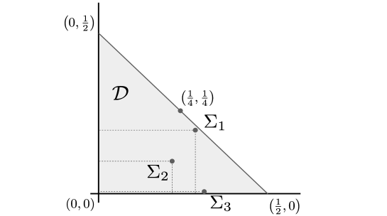
Figure 1: The covariance matrices $\Sigma_{1}$, $\Sigma_{2}$ and $\Sigma_{3}$ represented as functions of their eigenvalues in $\mathcal{D}$ (grey). The points $(0,0)$ and $(1/4,1/4)$ correspond to the minimum entropy and maximum entropy cases.

Consider the multivariate Bernoulli distributions $\mathbf{W}_{1}$, $\mathbf{W}_{2}$ and $\mathbf{W}_{3}$ with second order moments

$$\Sigma_{1}=\frac{1}{25}\begin{bmatrix}6&1\\ 1&6\end{bmatrix}, \Sigma_{2}=\frac{1}{625}\begin{bmatrix}66&-21\\ -21&126\end{bmatrix}, \Sigma_{3}=\frac{1}{625}\begin{bmatrix}66&91\\ 91&126\end{bmatrix}$$ and (36)

associated with two (increasingly correlated) arcs from networks. The eigenvalues of $\Sigma_{1}$, $\Sigma_{2}$ and $\Sigma_{3}$ are

$$\boldsymbol{\lambda}_{1}=\begin{bmatrix}0.28\\ 0.20\end{bmatrix}, \boldsymbol{\lambda}_{2}=\begin{bmatrix}0.2121\\ 0.095\end{bmatrix} \boldsymbol{\lambda}_{3}=\begin{bmatrix}0.3069\\ 0.0003\end{bmatrix}.$$ and (37)

The values of the generalized variance, total variance and squared Frobenius matrix norm (both normalized and in the original scale) for the three covariance matrices are reported int Table 1.

	$\mathsf{VAR}_{T}(\Sigma)$	$\mathsf{VAR}_{G}(\Sigma)$	$\mathsf{VAR}_{N}(\Sigma)$	$\overline{\mathsf{VAR}}_{T}(\Sigma)$	$\overline{\mathsf{VAR}}_{G}(\Sigma)$	$\overline{\mathsf{VAR}}_{N}(\Sigma)$
$\Sigma_{1}$	$0.48$	$0.056$	$0.1384$	$0.96$	$0.896$	$0.9642$
$\Sigma_{2}$	$0.3072$	$0.02016$	$0.2468$	$0.6144$	$0.32256$	$0.6752$
$\Sigma_{3}$	$0.3072$	$8.96\times 10^{-5}$	$0.2869$	$0.6144$	$0.00143$	$0.5682$

Table 1: Original and normalized values of $\mathsf{VAR}_{T}$, $\mathsf{VAR}_{G}$ and $\mathsf{VAR}_{N}$ for $\Sigma_{1}$, $\Sigma_{2}$ and $\Sigma_{3}$.

The corresponding asymptotic and Monte Carlo significance values are reported in Table 3 and 3 respectively. Each one has been computed for various hypothetical sample sizes ($m=10,20,50,100,200$). Parametric bootstrap has been performed on $R=10^{6}$ covariance matrices generated from the null distribution for each configuration of test statistic and sample size.

$t_{T}(\Sigma)$
	$10$	$20$	$50$	$100$	$200$
$\Sigma_{1}$	$0.491137$	$0.457610$	$0.405404$	$0.354943$	$0.291243$
	$\mathbf{0.906041}$	$\mathbf{0.863836}$	$\mathbf{0.781414}$	$\mathbf{0.691495}$	$\mathbf{0.571734}$
$\Sigma_{2}$	$0.094193$	$0.026330$	$0.000852$	$0.000003$	$0.000000$
	$\mathbf{0.173766}$	$\mathbf{0.049704}$	$\mathbf{0.001644}$	$\mathbf{0.000007}$	$\mathbf{0.000000}$
$\Sigma_{3}$	$0.094193$	$0.026330$	$0.000852$	$0.000003$	$0.000000$
	$\mathbf{0.173766}$	$\mathbf{0.049704}$	$\mathbf{0.001644}$	$\mathbf{0.000007}$	$\mathbf{0.000000}$
$t_{G_{2}}(\Sigma)$
$\Sigma_{1}$	$0.603944$	$0.524258$	$0.423183$	$0.341131$	$0.250054$
	$\mathbf{0.905218}$	$\mathbf{0.847522}$	$\mathbf{0.735799}$	$\mathbf{0.616696}$	$\mathbf{0.465129}$
$\Sigma_{2}$	$0.121488$	$0.023514$	$0.000278$	$0.000000$	$0.000000$
	$\mathbf{0.182091}$	$\mathbf{0.0380138}$	$\mathbf{0.000484}$	$\mathbf{0.000000}$	$\mathbf{0.000000}$
$\Sigma_{3}$	$0.000000$	$0.000000$	$0.000000$	$0.000000$	$0.000000$
	$\mathbf{0.000000}$	$\mathbf{0.000000}$	$\mathbf{0.000000}$	$\mathbf{0.000000}$	$\mathbf{0.000000}$
$t_{N}(\Sigma)$
$\Sigma_{1}$	$0.965205$	$0.909123$	$0.714937$	$0.436839$	$0.142271$
	$\mathbf{0.964547}$	$\mathbf{0.909108}$	$\mathbf{0.714937}$	$\mathbf{0.436839}$	$\mathbf{0.142271}$
$\Sigma_{2}$	$0.564938$	$0.253762$	$0.017090$	$0.000142$	$0.000000$
	$\mathbf{0.556708}$	$\mathbf{0.253636}$	$\mathbf{0.017090}$	$\mathbf{0.000142}$	$\mathbf{0.000000}$
$\Sigma_{3}$	$0.154551$	$0.014796$	$0.000008$	$0.000000$	$0.000000$
	$\mathbf{0.138557}$	$\mathbf{0.014628}$	$\mathbf{0.000008}$	$\mathbf{0.000000}$	$\mathbf{0.000000}$

Table 2: Asymptotic significance values of $t_{T}$, $t_{G_{2}}$ and $t_{N}$ for $\Sigma_{1}$, $\Sigma_{2}$ and $\Sigma_{3}$; the ones computed with the finite sample corrections are reported in bold.

$\overline{\overline{\mathsf{VAR}}}_{T}(\Sigma)$
	$10$	$20$	$50$	$100$	$200$
$\Sigma_{1}$	$0.569655$	$0.457109$	$0.129242$	$0.017416$	$0.000334$
$\Sigma_{2}$	$0.016834$	$0.000205$	$0$	$0$	$0$
$\Sigma_{3}$	$0.016834$	$0.000205$	$0$	$0$	$0$
$\overline{\overline{\mathsf{VAR}}}_{G}(\Sigma)$
$\Sigma_{1}$	$0.784102$	$0.512839$	$0.14788$	$0.013678$	$0.000094$
$\Sigma_{2}$	$0.063548$	$0.000761$	$0$	$0$	$0$
$\Sigma_{3}$	$0.005909$	$0.000008$	$0$	$0$	$0$
$\overline{\overline{\mathsf{VAR}}}_{N}(\Sigma)$
$\Sigma_{1}$	$0.743797$	$0.568819$	$0.239397$	$0.096544$	$0.019633$
$\Sigma_{2}$	$0.196996$	$0.037772$	$0.001018$	$0.000005$	$0$
$\Sigma_{3}$	$0.018292$	$0.000355$	$0$	$0$	$0$

Table 3: Bootstrap significance values of $\overline{\overline{\mathsf{VAR}}}_{T}$, $\overline{\overline{\mathsf{VAR}}}_{G}$ and $\overline{\overline{\mathsf{VAR}}}_{N}$ from parametric bootstrap for $\Sigma_{1}$, $\Sigma_{2}$ and $\Sigma_{3}$.

6 Comparing independence tests and structure learning algorithms

We will now illustrate how these tests can be used to compare different structure learning strategies, i.e. different combinations of structure learning algorithms, conditional independence tests and network scores. The impact of different choices for each component on the variability of the model can easily be assessed while keeping the other ones fixed.

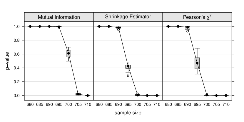
Figure 2: Significance values for three different conditional independence tests (asymptotic and shrinkage estimators of mutual information and Pearson’s $\chi^{2}$) used with the same structure learning algorithm (Grow-Shrink).

First we will compare the performance of the Grow-Shrink algorithm for three different conditional independence tests. The learning algorithm has been applied to samples of size $680$, $685$, $690$, $695$, $700$, $705$ and $710$ (20 for each size) generated from the ALARM reference network [33], which is composed by 37 discrete nodes and 46 arcs for a total of 509 parameters. Both the data and the software implementation of the algorithm are included in the bnlearn package [34] for R [35]. The following tests have been considered:

• the asymptotic $\chi^{2}$ test based on mutual information [23], which is in fact a log-likelihood ratio test and is also called the $G^{2}$ test [36].

• the shrinkage estimator for the mutual information, which is a James-Stein regularized estimator developed by Hausser and Strimmer [37].

• Pearson’s $\chi^{2}$ asymptotic test for independence [36].

The same threshold $\alpha=0.05$ for type I error has been used in three cases, and network variability has been assessed with the Monte Carlo test for the squared Frobenius norm.

Results are shown in Figure 2. All the tests considered in the analysis start producing relatively stable network structures – i.e. the null hypothesis corresponding to the maximum entropy case is rejected – at sample sizes $695$ and $700$. Pearson’s $\chi^{2}$ test performs slightly better than mutual information, as documented in Agresti [36] when dealing with sparse contingency tables. This is also true for the shrinkage estimator. However, the difference among the three sets of significance values is very small.

On the other hand we will now compare three different learning algorithms:

• TABU search (which is a score-based algorithm), combined with a Bayesian Information criterion (BIC) score.

• Grow-Shrink (which is a constraint-based algorithm) combined with the asymptotic $\chi^{2}$ test based on mutual information described above and $\alpha=0.05$.

• Max-Min Hill Climbing (which is hybrid algorithm), combined with a BIC score and the asymptotic mutual information test.

As can be seen in Figure 3 in this case differences are more pronounced. The Max-Min Hill Climbing algorithm, which is one of the top performers up to date for large networks, displays less variability than TABU search and Grow-Shrink at the same sample size. In particular the difference between Max-Min Hill Climbing and Grow-Shrink confirms the analysis made in Tsamardinos et al. [10] and the well-documented [3] instability displayed by constraint-based algorithms at small sample sizes.

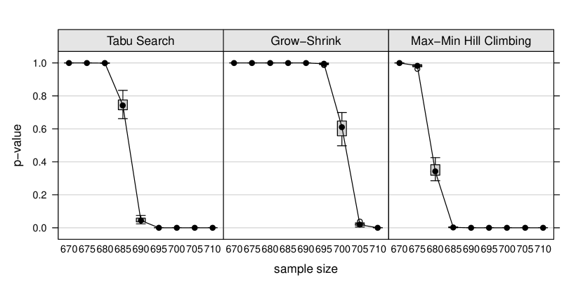
Figure 3: Significance values for three different structure learning algorithms (Grow-Shrink, TABU search and Max-Min Hill Climbing) using the same conditional independence tests and network scores (asymptotic mutual information test and the Bayesian Information Criterion (BIC), respectively).

7 Conclusions

In this paper we derived the properties of several measures of variability for the structure of a Bayesian network through its underlying undirected graph, which is assumed to have a multivariate Bernoulli distribution. Descriptive statistics, asymptotic and Monte Carlo tests were developed along with their fundamental properties. They can be used to compare the performance of different learning algorithms and to measure the strength of arbitrary subsets of arcs.

Appendix

Appendix A Bounds on the squared Frobenius matrix norm

The squared Frobenius matrix norm of the difference between the covariance matrix $\Sigma$ and the maximum entropy matrix $(1/4)I_{k}$ is

$$|||\Sigma-\frac{1}{4}I_{k}|||_{F}^{2}=\sum_{i=1}^{k}\left(\lambda_{i}-\frac{1}{4}\right)^{2}.$$ (38)

Its unique global minimum is zero for $\Sigma=(1/4)I_{k}$ but it has a varying number of global maxima depending on the dimension $k$ of $\Sigma$. They are the solutions of the constrained minimization problem

$$\min_{\mathcal{D}}f(\boldsymbol{\lambda})=-\sum_{i=1}^{k}\left(\lambda_{i}-\frac{k}{4}\right)^{2} \lambda_{i}\geqslant 0,\sum_{i=1}^{k}\lambda_{i}\leqslant\frac{k}{4}.$$ subject to (39)

This configuration of stationary points is not a problem for asymptotic and Monte Carlo tests, but prevents any direct interpretation of the values of descriptive statistics.

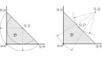
Figure 4: Squared Frobenius matrix norms from $(1/4)I_{K}$ (on the left) and $(k/4)I_{k}$ (on the right) in $\mathcal{D}$ for $k=2$. The green area is the set $\mathcal{D}$ of the possible eigenvalues of $\Sigma$ and the red lines are level curves.

On the other hand, the difference in squared Frobenius norm

$$\mathsf{VAR}_{N}(\Sigma)=|||\Sigma-\frac{k}{4}I_{k}|||_{F}^{2}=\sum_{i=1}^{k}\left(\lambda_{i}-\frac{k}{4}\right)^{2}$$ (40)

has both a unique global minimum (because it’s a strictly convex function)

$$\min_{\mathcal{D}}\mathsf{VAR}_{N}(\Sigma)=\mathsf{VAR}_{N}\left(\frac{1}{4}I_{k}\right)=\sum_{i=1}^{k}\left(\frac{1}{4}-\frac{k}{4}\right)^{2}=\frac{k(k-1)^{2}}{16}$$ (41)

and a unique global maximum

$$\max_{\mathcal{D}}\mathsf{VAR}_{N}(\Sigma)=\mathsf{VAR}_{N}(\mathbf{O})=\sum_{i=1}^{k}\left(\frac{k}{4}\right)^{2}=\frac{k^{3}}{16}$$ (42)

which correspond to the minimum entropy ($\boldsymbol{\lambda}=[0,\ldots,0]$) and the maximum entropy ($\boldsymbol{\lambda}=[1/4,\ldots,1/4]$) covariance matrices respectively (see figure 4). However since $(k/4)I_{k}$ is not a valid covariance matrix for a multivariate Bernoulli distribution, $\mathsf{VAR}_{N}(\Sigma)$ cannot be used to derive any probabilistic result.

Appendix B Multivariate Bernoulli and the maximum entropy case

The values of $p_{i}$ and $\Sigma$ in the maximum entropy case are a direct consequence from the following theorem.

Theorem 5.

Let $\mathcal{U}_{1},\ldots,\mathcal{U}_{n}$, $n=2^{m}$, $m=|\mathbf{V}|(|\mathbf{V}|-1)/2$ be all possible undirected graphs with vertex set $\mathbf{V}$ and let $\mathsf{P}(\mathcal{U}_{k})=1/n$, $k=1,\ldots,n$. Let $e_{i}$ and $e_{j}$, $i\neq j$ be two edges. Then $\mathsf{P}(e_{i})=1/2$ and $\mathsf{P}(e_{i},e_{j})=1/4$.

Proof.

The number of possible configurations of an undirected graph is given by the Cartesian product of the possible states of its $m$ edges, resulting in

$$|\{0,1\}\times\ldots\times\{0,1\}|=\left|\{0,1\}^{m}\right|=2^{m}$$ (43)

possible undirected graphs. Then edge $e_{i}$ is present in $2^{m-1}$ graphs and $e_{i}$ and $e_{j}$ are simultaneously present in $2^{m-2}$ graphs. Therefore

$$\mathsf{P}(e_{i})=\frac{2^{m-1}\mathsf{P}(\mathcal{U}_{k})}{2^{m}\mathsf{P}(\mathcal{U}_{k})}=\frac{1}{2} \mathsf{P}(e_{i},e_{j})=\frac{2^{m-2}\mathsf{P}(\mathcal{U}_{k})}{2^{m}\mathsf{P}(\mathcal{U}_{k})}=\frac{1}{4}.$$ and (44)

∎

The fact that $\sigma_{ij}=0$ for every $i\neq j$ also proves that the edges are independent according to Theorem 1.

References

References

- Friedman et al. [2000] N. Friedman, M. Linial, I. Nachman, Using Bayesian Networks to Analyze Expression Data, J. Comput. Biol. 7 (2000) 601–620.
- Holmes and Jain [2008] D. E. Holmes, L. C. Jain (Eds.), Innovations in Bayesian Networks: Theory and Applications, Springer-Verlag, Berlin, 2008.
- Spirtes et al. [2000] P. Spirtes, C. Glymour, R. Scheines, Causation, Prediction, and Search, MIT Press, Cambridge, 2000.
- Margaritis [2003] D. Margaritis, Learning Bayesian Network Model Structure from Data, Ph.D. thesis, School of Computer Science, Carnegie-Mellon University, Pittsburgh, PA, available as Technical Report CMU-CS-03-153, 2003.
- Tsamardinos et al. [2003] I. Tsamardinos, C. F. Aliferis, A. Statnikov, Algorithms for Large Scale Markov Blanket Discovery, in: Proc. of the 16th Int. Fla. Artif. Intell. Res. Soc. Conf., AAAI Press, Menlo Park CA, 376–381, 2003.
- Yaramakala and Margaritis [2005] S. Yaramakala, D. Margaritis, Speculative Markov Blanket Discovery for Optimal Feature Selection, in: Proc. of the 5th IEEE Int. Conf. on Data Mining, IEEE Computer Society, Washington DC, 809–812, 2005.
- Russell and Norvig [2009] S. J. Russell, P. Norvig, Artificial Intelligence: A Modern Approach, Prentice Hall, Upper Saddle River NJ, 3rd edn., 2009.
- Chickering [2002] D. M. Chickering, Optimal Structure Identification with Greedy Search, J. Mach. Learn. Res. 3 (2002) 507–554.
- Larrañaga et al. [1997] P. Larrañaga, B. Sierra, M. J. Gallego, M. J. Michelena, J. M. Picaza, Learning Bayesian Networks by Genetic Algorithms: A Case Study in the Prediction of Survival in Malignant Skin Melanoma, in: Proc. of the 6th Conf. on Artif. Intell. in Med. in Eur. (AIME’97), Springer, Berlin, 261–272, 1997.
- Tsamardinos et al. [2006] I. Tsamardinos, L. E. Brown, C. F. Aliferis, The Max-Min Hill-Climbing Bayesian Network Structure Learning Algorithm, Mach. Learn. 65 (1) (2006) 31–78.
- Elidan [2001] G. Elidan, Bayesian Network Repository, URL {http://www.cs.huji.ac.il/labs/compbio/Repository}, 2001.
- Jungnickel [2008] D. Jungnickel, Graphs, Networks and Algorithms, Springer-Verlag, Berlin, 3rd edn., 2008.
- Efron and Tibshirani [1993] B. Efron, R. Tibshirani, An Introduction to the Bootstrap, Chapman & Hall, New York, 1993.
- Friedman et al. [1999] N. Friedman, M. Goldszmidt, A. Wyner, Data Analysis with Bayesian Networks: A Bootstrap Approach, in: Proc. of the 15th Conf. on Uncertain. in Artif. Intell. (UAI-99), Morgan Kaufmann, San Fransisco, 206–215, 1999.
- Korb and Nicholson [2004] K. Korb, A. Nicholson, Bayesian Artificial Intelligence, Chapman and Hall, New York, 2004.
- Imoto et al. [2002] S. Imoto, S. Y. Kim, H. Shimodaira, S. Aburatani, K. Tashiro, S. Kuhara, S. Miyano, Bootstrap Analysis of Gene Networks Based on Bayesian Networks and Nonparametric Regression, Genome Inform. 13 (2002) 369–370.
- Krummenauer [1998a] F. Krummenauer, Limit Theorems for Multivariate Discrete Distributions, Metrika 47 (1) (1998a) 47–69.
- Krummenauer [1998b] F. Krummenauer, Efficient Simulation of Multivariate Binomial and Poisson Distributions, Biom. J. 40 (7) (1998b) 823–832.
- Ash [2000] R. B. Ash, Probability and Measure Theory, Academic Press, London, 2nd edn., 2000.
- Loève [1977] M. Loève, Probability Theory, Springer-Verlag, New York, 4th edn., 1977.
- Salce [1993] L. Salce, Lezioni sulle Matrici, Zanichelli, Padova, Italy, 1993.
- Bang-Jensen and Gutin [2009] J. Bang-Jensen, G. Gutin, Digraphs: Theory, Algorithms and Applications, Springer-Verlag, London, 2nd edn., 2009.
- Cover and Thomas [2006] T. A. Cover, J. A. Thomas, Elements of Information Theory, Wiley, Hoboken NJ, 2006.
- Muirhead [2005] R. J. Muirhead, Aspects of Multivariate Statistical Theory, Wiley, Hoboken NJ, 2005.
- Bilodeau and Brenner [1999] M. Bilodeau, D. Brenner, Theory of Multivariate Statistics, Springer-Verlag, New York, 1999.
- Mardia et al. [1979] K. V. Mardia, J. T. Kent, J. M. Bibby, Multivariate Analysis, Academic Press, London, 1979.
- Seber [2008] G. A. F. Seber, A Matrix Handbook for Stasticians, Wiley, Hoboken NJ, 2008.
- Nocedal and Wright [2006] J. Nocedal, S. J. Wright, Numerical Optimization, Springer, New York, 2nd edn., 2006.
- Anderson [2003] T. W. Anderson, An Introduction to Multivariate Statistical Analysis, Wiley, Hoboken NJ, 3rd edn., 2003.
- Steyn [1978] H. S. Steyn, On Approximations for the Central and Noncentral Distribution of the Generalized Variance, J. Am. Stat. Assoc. 73 (363) (1978) 670–675.
- Butler et al. [1992] R. W. Butler, S. Huzurbazar, J. G. Booth, Saddlepoint Approximations for the Generalized Variance and Wilks’ Statistic, Biometrika 79 (1) (1992) 157–169.
- Nagao [1973] H. Nagao, On Some Test Criteria for Covariance Matrix, Ann. Stat. 1 (4) (1973) 700–709.
- Beinlich et al. [1989] I. Beinlich, H. J. Suermondt, R. M. Chavez, G. F. Cooper, The ALARM Monitoring System: A Case Study with Two Probabilistic Inference Techniques for Belief Networks, in: Proc. of the 2nd Eur. Conf. on Artif. Intell. in Med., Springer-Verlag, Berlin, 247–256, 1989.
- Scutari [2010] M. Scutari, bnlearn: Bayesian network structure learning, URL http://www.bnlearn.com/, r package version 2.0, 2010.
- R Development Core Team [2010] R Development Core Team, R: A Language and Environment for Statistical Computing, R Foundation for Statistical Computing, Vienna, Austria, URL http://www.r-project.org, 2010.
- Agresti [2002] A. Agresti, Categorical Data Analysis, Wiley, Hoboken NJ, 2nd edn., 2002.
- Hausser and Strimmer [2009] J. Hausser, K. Strimmer, Entropy Inference and the James-Stein Estimator, with Application to Nonlinear Gene Association Networks, J. Mach. Learn. Res. 10 (2009) 1469–1484.