Dynamics on Spatial Networks and the Effect of Distance Coarse graining

Abstract

Very recently, a kind of spatial network constructed with power-law distance distribution and total energy constriction is proposed. Moreover, it has been pointed out that such spatial networks have the optimal exponents $\delta$ in the power-law distance distribution for the average shortest path, traffic dynamics and navigation. Because the distance is estimated approximately in real world, we present an distance coarse graining procedure to generate the binary spatial networks in this paper. We find that the distance coarse graining procedure will result in the shifting of the optimal exponents $\delta$. Interestingly, when the network is large enough, the effect of distance coarse graining can be ignored eventually. Additionally, we also study some main dynamic processes including traffic dynamics, navigation, synchronization and percolation on this spatial networks with coarse grained distance. The results lead us to the enhancement of spatial networks’ specifical functions.

I Introduction

The research on complex networks has been one of the most active fields not only in physics but also in other various disciplines of natural and social sciencesRMP47 ; Nature440 ; Science509 ; RMP75 . In traditional statistical mechanics, interaction mainly exists between neighboring elements. By introducing the complex topology of the networks, the whole system can emerge some new properties such as small-worldNature440 , scale-free degree distributionScience509 and community structuresRMP75 . However, the spatial property is of great significance as well, which makes the interaction between nodes go beyond the neighboring effect but under the restraint of their underlying geographical site. This property matters much in lots of empirical networks including neural networkComplexity56 , communication networksPRE015103 , the electric-power gridPRE025103 , transportation systemsPNAS7794 ; PRE036125 ; PhysicaA109 and even social networksSocial187 ; PhysicaA5317 ; PNAS11623 ; arxiv1802 ; arxiv1332 . Generally, the geography information of the nodes and the distance between nodes in these networks would determine the characteristics of the network and play an important role in the dynamics happening in the network.

About the networks embedded in the geographical space, many works has been doneFC1994 ; PNAS13382 ; PRE037102 ; PRE026118 ; PhysicaA853 ; EPJB1434 ; PRE016117 . The first category is focusing on the spatial distribution of the nodes of these empirical spatial networksFC1994 ; PNAS13382 . Specifically, networks with strong geographical constraints, such as power grids or transport networks, are found with fractal scalingFC1994 . Besides, others researchers discussed the small-world behavior and the scale-free networks in Euclidean spacePRE037102 ; PRE026118 . For example, when supplementing long range links whose lengths are distributed according to $q(l)\propto l^{-\alpha}$ to D-dimensional lattices, Sen, Banerjee and Biswas conjectured that the two transition points from random networks and Regular networks to the networks with small-world effect in any dimension are: $\alpha=D$ and $\alpha=D+1$ respectivelyPRE037102 . Also, Xulvi-Brunet and Sokolov constructed an growing network model by $\prod\limits_{i\rightarrow j}\propto k_{i}l_{ij}^{-\alpha}$, where $l_{ij}$ is the distance between $i$ and $j$. Numerical simulations have shown that for $\alpha<1$ the degree distribution is a power-law distribution and for $\alpha>1$ it is fitted by a stretched exponentialPRE026118 . In addition, some researchers also introduced some ways to model the empirical geographical networksPhysicaA853 ; EPJB1434 ; PRE016117 ; arxiv1332 .

However, few of these former works in spatial networks are related to the total cost restraint. In fact, The total cost is very important when designing these real spatial networks. Because the longer a link is, the more it will cost. Very recently, some researches took this aspect into accountEPL58002 ; PRL018701 ; arxiv1802 . In EPL58002 , based on a regular network and subject to a limited cost $C$, long range connections are added with power-law distance distribution under the probability density function (PDF) $P(r)=ar^{-\delta}$. Some basic topological properties of the network with different $\delta$ are studied. It is found that the network has the minimum average shortest path when $\delta=2$ in one-dimensional spatial networks, In addition, the authors investigated a classic traffic model on this model networks. It is found that $\delta=1.5$ is the optimization value for the traffic process on the spatial networks. In PRL018701 , pairs of sites $ij$ in 2-dimensional lattices are randomly chosen to receive long-range connections with probability $Pr(u,v)$ proportional to $r_{uv}^{-\alpha}$. With the total energy restriction, G. Li et cl. found $\alpha=3$ is corresponding to the minimum average shortest path. Moreover, they claimed that the optimal value for navigation is $\alpha=3$ in 2-dimensional spatial networks and $\alpha=2$ in 1-dimensional onesexplain .

In many empirical researches, especially the study on traffic networks, the distances are estimate approximatelyPNAS7794 ; PRE036125 ; PhysicaA109 ; PhysicaA5639 . That is to say scientists incline to regard a range of distance as a typical value. This procedure named distance coarse graining should also be studied in the spatial network models. Actually, the coarse graining process has been discussed since long times agoPRL168701 ; PRL038701 ; PRL174104 ; PhysicaA5639 . All the related works focus on how to reduce the size of the networks while keep other properties unchanged such as degree distribution, cluster coefficient, degree correlationPRL168701 , random walksPRL038701 and synchronizabilityPRL174104 . On the other hand, the probability distribution of these long range-connections is chosen as $P(r)=ar^{-\delta}$ in the spatial network. It means most of the connections are short while a few connections are relatively long. However, each node has only two neighbors. When the total cost constraint is chosen as a certain large value in the binary network, the network can not provide enough short long-range connections. In this paper, we use the distance coarse graining to solve this problem. Specially, we will study how the distance coarse graining affects the topology and dynamical process in the spatial network model. The result shows that the $\delta$ for minimum average shortest path, optimal traffic processPRE026125 ; PRE046108 and navigationNature845 ; PRE017101 ; PRL238703 ; PhysicaA109 will shift to smaller value. And the more we coarse grain the distance, the more significantly the optimal $\delta$ will shift. Interestingly, when the network is large enough, the effect of distance coarse graining can be ignored. In other aspect, how the dynamic processes perform in spatial networks is an interesting problem but hasn’t received enough attention. Investigating the dynamics on the spatial networks can not only lead to enhancement of the function of the spatial network but also provide us with a better understanding of it. Here, we study two more main dynamic processes and find synchronizabilityEPL48002 ; PR93 can also be optimized by a typical $\delta$ while there is no optimal $\delta$ for percolationRMP1275 in such spatial network model.

II Generating Binary Spatial Networks with Coarse Grained Distance

The model network is embedded in a $k$-dimensional regular network. The long range connections is generated from a power-law distance distribution. A total cost $C$ is introduced to this network model. Every edge has a cost $c$ which is linear proportion to its distance $r$. For simplification, the edge connecting node $i$ and $j$ cause a cost represented by its length $r_{ij}$ in the model.

According to many empirical studies, the distance obeys the power-law distributionIPSJ155 ; GeoJournal102 ; Social187 ; PhysicaA5317 ; PNAS11623 . Specially, for Japanese airline networks, even there is an exponential decay in domestic flights, the distance distribution follows power-law when international flights are addedIPSJ155 . For the U.S. intercity passenger air transportation network, the distribution of the edge distance has a power-law tail with the exponent $\delta=2.20\pm 0.19$GeoJournal102 . Additionally, authors in ref.Social187 ; PhysicaA5317 ; PNAS11623 found $\delta=1$ for social systems like the mobile phone communication networks. Therefore, the probability distribution of these long range connections here is chosen as $P(r)=ar^{-\delta}$ (PDF) in the spatial model. In order to coarse grain the distance, when adding a long range link to the network, we divide the distance into many continuous parts in which all the distances are considered as one typical value. So the spatial network is constructed as following:

1. $N$ nodes are arranged in a $1$-dimensional lattice. Every node is connected with its nearest neighbors which can keep every node reachable. Additionally, between any pair of nodes there is a well defined lattice distance.

2. Set the approximate interval $W$ of coarse graining process. For each node, divide the distance between it and other nodes into $\frac{N_{max}}{W}$ parts ($N_{max}$ is the largest distance between any nodes in the initial network), the $m$th part are $(m-1)W+1$,$(m-1)W+2$,…,$mW$.

3. A node $i$ is chosen randomly, and a certain distance $r(2\leq r\leq N_{max}$) is generated with probability $P(r)=ar^{-\delta}$, where $a$ is determined from the normalization condition $\sum^{N_{max}}_{r=2}P(r)=1$.

4. Find the part that the distance $r$ belongs to, say $m$th part here. Then, one of the nodes in this part is picked randomly, for example node $j$. An edge between nodes $i$ and $j$ is created if there exists no edge between them yet.

5. After step $4$, a certain cost $r_{ij}$ is generated. Repeat step $3$ and $4$ until the total cost reaches $C$.

Obviously, there are two significant features of the spatial network: the power-law distribution of the long range connections in the network and the restriction on total energy. Firstly, we should determine how to choose an appropriate $W$ under different total cost $C$. In the spatial network, the probability distribution of these long range-connections is chosen as $P(r)=ar^{-\delta}$. It means most of the connections are short while a few connections are relatively long. However, each node has only two neighbors. When the total cost reaches a certain value in the binary network, the short range part of the network would become nearly full connected and can not provide further short long-range connections. Consequently, binary spatial network can not be generated directly without the distance coarse grained. Clearly, if $W$ is too small, the spatial network model still can not provide enough short long-range connections. On the contrary, because all the nodes in one distance coarse graining part are regarded as the same, if $W$ is too large, too many nodes are considered in one distance coarse graining part so that the power-law distance distribution will be destroyed significantly.

In order to deduce the formula of appropriate $W$, we consider an extreme condition with $\delta$ equaling to a very large positive value. Under this circumstance, all the long-range connections are short. So all of them will locate in the first distance coarse graining part of each node. Consequently, the total energy is $C=(2+3+4+...+W)N$. For $C=cn$, $2+3+4+...+W=c$ where $c$ is the average energy on each node. After simplification, $W^{2}+W-2-2c=0$. So we can get $W=\frac{\sqrt{9+2c}-1}{2}$. Generally, $W$ only has to obey $W\geq[\frac{\sqrt{9+2c}-1}{2}]_{floor}$ where the $[\cdot]_{floor}$ represents the operation of rounding downward. In this paper, we choose $W=4$ when $c=10$, $W=7$ when $c=30$ and $W=9$ when $c=50$.

As mentioned above, the binary spatial network can not be generated directly. In refEPL58002 , to get the binary spatial network, authors project the weighted spatial network into unweighted one by imposing all the weight of the existing links to $1$, this will lead to losing total energy. On the contrary, when the distance is coarse grained, the network can provide enough short-term links. Under this circumstance, the binary spatial network can be generated independent from the weighted one. In Fig.1, we compare the total energy of these two different binary spatial networks. Clearly, only the network with coarse grained distance can satisfy the total energy limit as the standard value.

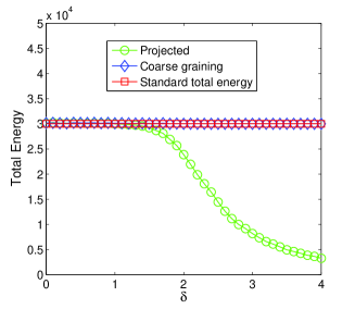
Figure 1: (Color online) The total energy of two different binary spatial networks. The cycle represents the projected binary spatial networks in ref.[11]. The lozenge stands for the binary spatial network with coarse grained distance with $W=7$. The square is the standard total energy which equals $C=n\times c=1000\times 30=30000$. The results are under 100 independent realization.

For the power-law distance distribution, just like we discussed above, there is no doubt that it will be destroyed when the distance is coarse grained. The results for distance distribution is reported in Fig.2. We can see that the distance distribution in projected binary spatial networks are almost the same as the standard distance power-law distribution. On the contrary, in networks with coarse grained distance, the distribution is different from the standard one. This is reasonable, because the node in each coarse grained part are regarded homogeneous. Consequently, the distribution plot is also divided into some continuous parts in which the distance distribution is normal. However, when we estimate the distance with higher scale, which means marking all the distance from $(m-1)W+1$ to $mW$ as a specific value $(m-1)W+1$, the distance distribution become exactly the same with the standard power-law, see the green line in Fig.2.

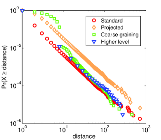
Figure 2: (Color online) Distance distribution of two different spatial networks. The lozenge represents result of the projected binary spatial networks in ref.[11]. The square stands for the distance distribution under original scale of the binary spatial network with coarse grained distance $W=7$. The triangle is the distance distribution under higher scale (See the text) of the coarse grained network. The cycle is the standard distance power-law distribution with given $n=10000$, $c=30$ and $\delta=3$. The results are under 10 independent realization.

One of the most important results in the former works about spatial networks is that the minimum shortest path happens at $\delta=2$ regardless of the total energyEPL58002 ; PRL018701 . Here, we investigate how the optimal $\delta$ changes as the distance coarse graining procedure. Fig.3 shows the result for three different level of distance graining. Obviously, the larger $W$ we choose to coarse grain the distance, the more severely the optimal point shifts to a lower value. However, as the size of the network is getting bigger, the shifting effect of the distance coarse graining becomes less significant. That is to say, notwithstanding the coarse graining in distance, the $\delta$ for the minimum shortest path still equals to $2$ in large networks.

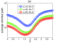
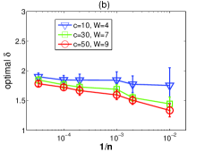
Figure 3: (Color online) The result for how the optimal $\delta$ changes as the distance coarse graining procedure. (a) is the average shortest path length for different $\delta$ under different coarse graining scale, here $N=1000$. (b) is how the $\delta$ for minimum average shortest path changes when the network getting larger. The results are under 100 independent realization.

III The dynamics on spatial networks and the effect of distance coarse graining

Dynamics on spatial networks is an interesting topic, for example, it can help us obtain the principle to design the optimal transportation networksPRL018701 . In this section, some main dynamics process will be studied on the spatial networks. Furthermore, most of the time, people tend to coarse grain the distance when designing the real networks, especially these transport networks. So understanding how the distance coarse graining affects the function of the network can be not only of great interest but also useful. So we will also discuss the effect of distance coarse graining on the function of spatial networks. Firstly, based on the results in the former worksEPL58002 ; PRL018701 , we know that the spatial properties of the network will result in optimal $\delta$ for navigation and traffic process respectively. So how the optimal $\delta$ shifts with the distance coarse graining procedure will be investigated. Secondly, we will study the synchronizability in this so-called binary spatial network with distance coarse grained. Finally, the percolation performance in this binary spatial network will be studied as well.

III.1 The Effect on Traffic Process

In traffic processPRE026125 , All the nodes embedded on the spatial network are treated as both hosts and routers. Every node can deliver at most $D$ packets one step toward their destinations. At each time step, there are $R$ packets generated homogeneously on the nodes in the system. The packets are delivered from their own origin nodes to destination nodes by special routing strategy. There is a critical value $R_{c}$ which can best reflect the maximum capability of a system handling its traffic. In particular, for $R<R_{c}$, the numbers of created and delivered packets are balanced, leading to a steady free traffic flow. For $R>R_{c}$, traffic congestion occurs as the number of accumulated packets increases with time, simply because the capacities of the nodes for delivering packets are limited.

In fact, the whole traffic dynamics can be represented by analyzing the largest betweenness of the networkPRE046108 . The betweenness of a node is the number of shortest path passing through this node. Note that with the increasing of parameter $R$ (number of packets generated in every step), the system undergoes a continuous phase transition to a congested phase. Below the critical value $R_{c}$, there is no accumulation at any node in the network and the number of packets that arrive at node $i$ is $Rg_{i}/N(N-1)$ on average. Therefore, a particular node will collapse when $Rg_{i}/N(N-1)>D_{i}$, where $g_{i}$ is the betweenness coefficient and $D_{i}$ is the transferring capacity of node $i$. Therefore, congestion occurs at the node with the largest betweenness. Thus $R_{c}$ can be estimated as $R_{c}=D_{i}N(N-1)/g_{max}$, where $g_{max}$ is the largest betweenness coefficient of the network.

Here, we study the traffic dynamics in the spatial network with coarse grained distance. The results are given in Fig.4(a) and (b). In Fig.4(a), it is quite obvious that there exists an optimal $\delta$ for $Rc$, which means the transport capacity reaches its maximum in this spatial networks. From Fig.4.(b), we can clearly see that this optimal $\delta$ gets closer to $1.5$ gradually as the size of the network becomes larger. Actually, even losing the total energy, the projected spatial network also has the optimal $\delta$ for traffic process equalling to $1.5$ in ref.EPL58002 . This implies that the spatial property play an dominative part in the traffic dynamics.

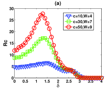
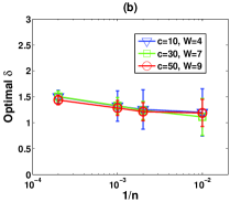
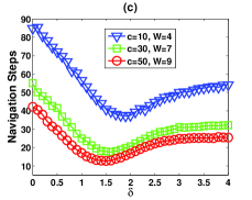
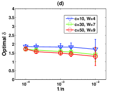
Figure 4: (Color online) The effect of distance coarse graining on the function of the binary spatial networks. (a) is the critical value $Rc$ in traffic process for different $\delta$ under different coarse graining scale, where $N=1000$. (b) shows how the optimal $\delta$ for traffic process changes when the network gets larger. (c) is the navigation steps for different $\delta$ under different coarse graining scale, where $N=1000$. (d) shows how the optimal $\delta$ for navigation changes when the network gets larger. The results are under 50 independent realization.

III.2 The Effect on Navigation

Another aspect we are going to investigate here is navigation. In fact, the navigation process in networks is based on local information, which is different from the shortest path with global information. Hence, the navigation reflects another ability of the networks. According to ref.PRL018701 , we choose the navigation strategy as the greedy algorithmNature845 in this paper. In the former works, Kleinberg found that $\alpha=2$ for $Pr(u,v)\propto r_{uv}^{-\alpha}$ is the optimal value in the navigation with the greedy algorithm in 2-dimensional spatial networks without total energy limitNature845 . When adding the energy restriction, G. Li et cl. found that the optimal value is $\alpha=3$ in 2-dimensional spatial networks and $\alpha=2$ in 1-dimensional onesPRL018701 .

Here, though we choose the PDF of the distance distribution as $P(r)=ar^{-\delta}$, $\delta$ equals to $\alpha$ in one-dimensional spaceexplain . What interest us most is that how this optimal value performs when the distance is coarse grained. In Fig.4 (c) and (d), the results are given. The optimal $\delta$ shifts to a smaller value as the coarse grained interval $W$ gets larger. However, when the size of the networks is large enough, the optimal $\delta$ will come back to $2$ even if the distance gets coarse grained, as show in Fig.4(d).

III.3 The Effect on Synchronizability

Furthermore, we will study the synchronizability in this so-called binary spatial network with distance coarse grained. The synchronization is a universal phenomenon emerged by a population of dynamically interacting units. It plays an important role from physics to biology and has attracted much attention for hundreds of years.

In the former works, the analysis of Master Stability Function (MSF) allows us to use the eigenratio $R=\lambda_{N}/\lambda_{2}$ of the Laplacian matrix to represent the synchronizability of a networkPR93 . Hence, we can calculate the synchronizability $R$ under different $\delta$. In Fig.5, synchronizability of the spatial network is enhanced in some specifical exponent $\delta$. Likewise, there is also an optimal $\delta$ for synchronizability which is $1.5$ approximately when the network is large enough.

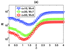
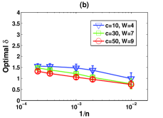
Figure 5: (Color online) The effect of distance coarse graining on the synchronizability of the binary spatial networks. (a) is the synchronizability $R$ for different $\delta$ under different coarse graining scale, where $N=1000$. (b) shows how the optimal $\delta$ for synchronizability changes when the network gets larger. The results are under 50 independent realization.

III.4 The Effect on Percolation

We have known that there are two different ways to obtain the binary spatial networks. The first is to project the weighted spatial networks to an binary one, the second is to generate the binary spatial networks directly by distance coarse graining procedure. To begin with, we compared the percolation performance of the these two kinds of networks. In percolation, we consider what happens with a network if a random fraction $1-p$ of its edges is removed. In this bond percolation problem, the giant connected component plays the role of the percolation cluster, which may be destroyed by decreasing $p$RMP1275 . Obviously, different $\delta$ in spatial networks will result in different critical parameter $p_{c}$. The smaller the critical parameter $p_{c}$ is, the better the networks perform in percolation. The results for the percolation performance of the these two kinds of binary spatial networks are shown in Fig.6.

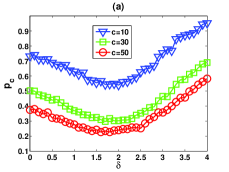
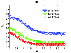
Figure 6: (Color online) The results for the percolation performance of (a)projected binary spatial networks and (b) coarse grained binary spatial networks. Here, the network size is $N=500$. The results are under 50 independent realization.

From Fig.6, we can see that the projected binary spatial networks have an optimal $\delta$ for percolation while coarse grained binary spatial networks do not. Actually, when projecting the weighted spatial networks, lots of energy gets lost. So in the projected binary spatial, the number of total links become smaller as $\delta$ gets largerEPL58002 . This is why the projected binary spatial networks have an optimal $\delta$ for percolation. Actually, when designing the binary spatial network, it is supposed to constrained by the total cost. In the percolation, we show that adding the total energy constraint by the distance coarse graining, the spatial network may perform entirely different in some functions. It indicates the distance coarse graining is necessary when analyzing some dynamics on spatial networks.

IV Conclusion

The complex networks has been a hot topic in science for more than ten years. Works in this field are based on the topology of the networks. So far, many empirical works claim that the distance distribution of real networks obeys power-law distribution. In theoretical modeling aspect, researches begin to pay attention to these spatial networks. Very recently, these spatial networks are constructed with power-law distance distribution and under total energy restriction. This kind of spatial networks can reflect the trade off property of real networks between the efficiency (distance power-law distribution) and the total cost.

Studying the dynamic on spatial networks is of great significance, which can lead to the enhancement of networks’ specifical function by choosing the proper exponent $\delta$. In previous works, authors found that there exist stable optimal power-law indexes $\delta$ for minimum shortest path, traffic process and navigation. With these understandings, people may obtain the principle to design the effective transport networks. In this paper, we study the percolation and synchronizability in such binary spatial networks with coarse grained distance. we find that synchronizability can also be optimized by a typical $\delta$ while no optimal $\delta$ exists for percolation in such spatial network model.

In most case of real lives and empirical researches, the distances are estimate approximately. In other words, people incline to regard a range of distance as a typical distance. How this coarse graining procedure affects the optimal $\delta$ is also studied in this paper. Our results show that the distance coarse graining procedure will make the optimal exponent $\delta$ in power-law distance distribution shift to smaller values for all of average shortest path, traffic process and navigation. Interestingly, when the network is large enough, the effect of distance coarse graining can be ignored. As the real networks, say the transport networks, is usual of relatively large size, the result indicates that the optimal index $\delta$ still works in designing principles for the optimal real transport networks. These results above indicate that the distance coarse graining can be used as a universal way to generate the binary spatial model with its total cost constraint satisfied and its power-law distance distribution preserved effectively. Moreover, investigation of functions of spatial related networks with coarse grained distance can be an interesting extension.

References

- (1) R. Albert and A.-L. Barabasi, Rev. Mod. Phys. 74, 47 (2002).
- (2) D. J. Watts and S. H. Strogatz, Nature 393, 440 (1998).
- (3) R. Albert and A.-L. Barabasi, Science 286, 509 (1999).
- (4) S. Fortunato, Rev. Mod. Phys. 486, 75 (2010).
- (5) O. Sporns, Complexity 8, 56 (2002).
- (6) V. Latora and M. Marchiori, Phys. Rev. E 71, 015103 (2005).
- (7) R. Albert, I. Albert and G. L. Nakarado, Phys. Rev. E 69, 025103 (2004).
- (8) R. Guimera, S. Mossa, A. Turtschi and L. A. N. Amaral, Proc. Natl. Acad. Sci. 102, 7794 (2005).
- (9) P. Crucitti, V. Latora and S. Porta, Phys. Rev. E 73, 036125 (2006).
- (10) V. Latora and M. Marchiori, Physica A 314, 109 (2002).
- (11) L. Adamic and E. Adar, Social Networks 27, 187 (2005).
- (12) R. Lambiottea, V. D. Blondela, C. de Kerchovea, E. Huensa, C. Prieurc, Z. Smoredac and P. V. Doorena, Physica A 387, 5317 (2008).
- (13) D. Liben-Nowell, J. Novak, R. Kumar, P. Raghavan and A. Tomkins, Proc. Natl. Acad. Sci. 102, 11623 (2005).
- (14) Y. Hu, Y. Wang, D. Li, S. Havlin and Z. Di, arXiv:1002.1802v1.
- (15) Y. Hu, D. Luo, X. Xu, Z. Han and Z. Di, arXiv:1002.1332v1.
- (16) M. Batty, P. Longley, Fractal Cities, Academic Press, New York, (1994).
- (17) S.-H. Yook, H. Jeong, A.-L. Barab si, Proc. Natl. Acad. Sci. USA 99, 13382 (2002).
- (18) P. Sen, K. Banerjee, T. Biswas, Phys. Rev. E 66, 037102 (2002).
- (19) R. Xulvi-Brunet, I.M. Sokolov, Phys. Rev. E 66, 026118 (2002).
- (20) P. Crucitti, V. Latora, S. Porta, Physica A 369, 853 (2006).
- (21) M.T. Gastner and M.E.J. Newman, European Physical Journal B 49, 1434(2004).
- (22) M.T. Gastner and M.E.J. Newman, Phys. Rev. E 74, 016117 (2006).
- (23) H. Yang, Y. Nie, A. Zeng, Y. Fan, Y. Hu and Z. Di, Europhys. Lett. 89, 58002 (2010).
- (24) Actually, probability of two nodes (u and v) to have a long range connection is different from the probability density function (PDF) of the distance distribution. Specifcally, in 1-dimensional space, . in 2-dimensional space, the number of nodes which have distance from a given node is proportional to , so the PDF is .
- (25) G. Li, S. D. S. Reis, A. A. Moreira, S. Havlin, H. E. Stanley and J. S. jr. Andrade, Phys. Rev. Lett. 104, 018701 (2010).
- (26) B. J. Kim, Phys. Rev. Lett. 93, 168701 (2004).
- (27) D. Gfeller and P. D. Los Rios, Phys. Rev. Lett. 99, 038701 (2007).
- (28) D. Gfeller and P. D. Los Rios, Phys. Rev. Lett. 100, 174104 (2008).
- (29) R. Wang, J.X. Tan, X. Wang, D.J. Wang and X. Cai, Physica A 387, 5639 (2008).
- (30) L. Zhao, Y.-C. Lai, K. Park and N. Ye, Phys. Rev. E 71, 026125 (2005).
- (31) G. Yan, T. Zhou, B. Hu, Z.Q. Fu and B.H. Wang, Phys. Rev. E 73, 046108 (2006).
- (32) J. M. Kleinberg, Nature 406, 845 (2000).
- (33) M. R. Roberson and D. ben-Avraham, Phys. Rev. E 74, 017101 (2006).
- (34) C. C. Cartozo and P. D. Los Rios, Phys. Rev. Lett. 102, 238703 (2009).
- (35) Y. Hayashi, IPSJ Digital Courier, 2, 155 (2006).
- (36) Z. Xu and R. Harriss, GeoJournal, 73, 102 (2008).
- (37) J. M. Kleinberg, Nature (London) 406, 845 (2000).
- (38) A. Zeng, Y. Hu and Z. Di, Europhys. Lett. 87, 48002 (2009).
- (39) A. Arenas, A. Diaz-Guilera, J. Kurths, Y. Morenob and C. Zhou, Phys. Rep. 469, 93 (2008).
- (40) S. N. Dorogovtsev and A. V. Goltsev, Reviews of Modern Physics 80, 1275 (2008).