Hot carriers in a bipolar graphene

Abstract

Hot carriers in a doped graphene under dc electric field is described taking into account the intraband energy relaxation due to acoustic phonon scattering and the interband generation-recombination transitions caused by thermal radiation. The consideration is performed for the case when the intercarrier scattering effectively establishes the quasiequilibrium electron-hole distributions, with effective temperature and concentrations of carriers. The concentration and energy balance equations are solved taking into account an interplay between weak energy relaxation and generation-recombination processes. The nonlinear conductivity is calculated for the momentum relaxation caused by the elastic scattering. The current-voltage characteristics, and the transition between bipolar and monopolar regimes of conductivity are obtained and analyzed, for different temperatures and gate voltages.

I Introduction

Study of the heated under dc electric field nonequilibrium carriers in graphene is stimulated by attempts of realization of efficient field-effect transistor, see 1 and Refs. therein. Essential heating also takes place for the cleaning of graphene by strong pulses of applied current 2 and in recent measurements, 2a conducted in electric fields $E\geq$1 kV/cm. In addition, excited by ultrafast interband pumping electron-hole pairs are actively studied 3 . In connection with such experiments theoretical studies of energy relaxation, both analytical 4 and numerical 5 , were conducted as well as studies of relaxation dynamics after ultrafast photoexcitation 6 . Recently, investigation of carriers heating under dc electric field applied to an intrinsic graphene has been given in 7 . Main peculiarities of the processes of heating in graphene (gapless and massless semiconductor, which is described by the Weyl-Wallace model 8 ) are related with an interplay between quasi-elastic energy relaxation on acoustic phonons and generation-recombination processes, that are effective nearby the cross point of energy spectrum. In a gated graphene, when monopolar regime of transport is realized, contribution of generation-recombination processes is suppressed. Effect of the gate voltage on the processes of carriers heating and on current-voltage characteristics of a gated graphene (i.e., a study of the model of field transistor located on graphene sheet of large dimensions) have not been considered so far.

In this paper a heating of carriers in doped graphene is analyzed theoretically, for the case when difference between the densities of electrons and holes is controlled by a gate voltage. Present treatment is limited by the region of energies below the energy of optical phonon ($\omega_{o}\approx 0.2$eV), when it is necessary to take into account the Joule heating produced by dc current, induced by electric field E, as well as following processes of relaxation: a) elastic relaxation of momentum due to elastic scattering on structural disorder 9 , which is the most effective mechanism of scattering so that anisotropy of carriers distributions is small; b) quasi-elastic relaxation of energy on acoustic phonons; and c) generation-recombination processes for interband transitions caused by thermal radiation (relaxation of energy and concentrations were analyzed for photoexcitation in 10 ). Here we consider the regime when the interparticle Coulomb scattering dominates over the processes of relaxation of the energies and the concentrations, so that the carriers are described by quasiequilibrium distributions with effective temperature and nonequilibrium concentrations of electrons and holes. These parameters are defined from the balance equations of the concentrations and the total energy, where the areal charge density of graphene sheet, given by the difference of the electron and the hole densities, is controlled by gate voltage. Besides determination of the average energies of carriers and their concentrations, nonlinear current-voltage characteristics are also studied below.

The analysis performed below is organized as follows. The basic equations, describing heating of carriers in gated graphene are evaluated in Sec. II. Results of calculations, including the parameters of quasiequilibrium distributions, nonequilibrium concentrations and current-voltage characteristics as a function of applied field, gate voltage, and temperature are presented in Sec. III. Discussion of the assumptions used and concluding remarks are given in Sec. IV. In Appendix the collision integrals used in present treatment are specified.

II Basic equations

Our description of the heating of bipolar plasma in graphene under dc electric field is based on quasiclassical kinetic equations that take into account the scattering mechanisms listed above. Here we assume that $\nu_{m}\gg\nu_{cc}\gg\nu_{qe,r}$, where $\nu_{m}$, $\nu_{cc}$, and $\nu_{qe}$ ($\nu_{r}$) are the relaxation frequencies of momentum, intercarrier scattering, and energy (concentration), respectively. Due to dominance of the relaxation of momentum, the weak anisotropic contributions to the electron ($e$) and the hole ($h$) distributions are given as 9

$$\Delta f_{k{\bf p}}=\pm\frac{(e{\bf E}\cdot{\bf p})}{p\nu_{p}^{(m)}}\left(-\frac{df_{kp}}{dp}\right).$$ (1)

Here $k=e$ ($k=h$) corresponds the upper (lower) sign and the frequency of momentum relaxation $\nu_{p}^{(m)}=v_{m}p\Psi(pl_{c}/\hbar)/\hbar$ is expressed by means of the characteristic velocity $v_{m}$ (that defines efficiency of scattering), and of the truncation factor for long-range scattering 9 $\Psi(x)=x^{-2}\exp(-x^{2})I_{1}(x^{2})$. Here the correlation length of static disorder, $l_{c}$, and the modified Bessel function of the first kind, $I_{1}(x)$, are used. The nonequilibrium isotropic distributions $f_{kp}$ are defined by kinetic equations

$$\pm\overline{e{\bf E}\cdot\frac{\partial\Delta f_{kp}}{\partial{\bf p}}}=J_{qe}\left(f|kp\right)+J_{r}\left(f|p\right)+J_{cc}\left(f|kp\right),$$ (2)

where an overline stands for the averaging over the angle in ${\bf p}$-plane. The collision integrals in the right hand side of Eq. (2) are given in Appendix.

Obtained from Eq. (2) distributions $f_{kp}$ define concentrations of electrons, $n_{e}$, and holes, $n_{h}$, as follows

$$n_{k}=4\int\frac{d{\bf p}}{(2\pi\hbar)^{2}}f_{kp},$$ (3)

where the factor $4$ takes into account degeneration over the spin and the valleys. The current density, I, is given as

$${\bf I}=4e\int\frac{d{\bf p}}{(2\pi\hbar)^{2}}{\bf v}_{\bf p}\left(\Delta f_{e{\bf p}}-\Delta f_{h{\bf p}}\right),$$ (4)

where ${\bf v}_{\bf p}=v_{W}{\bf p}/p$ is the velocity of particle with momentum p, written using the characteristic velocity $v_{W}\approx 10^{8}$cm/s. The sheet charge is defined by the difference of concentrations $n_{e}-n_{h}\equiv\Delta n_{s}$ that is controlled by the gate voltage $V_{g}$ applied to the back gate, placed at a distance $d$ from the graphene sheet. Considering such structure as plane capacitor, we obtain relation between $\Delta n_{s}$ and $V_{g}$ as follows: $\Delta n_{s}=\epsilon V_{g}/(4\pi|e|d)$, where $\epsilon\approx 3$ is dielectric constant of SiO₂ substrate.

Because of predominance of the intercarrier scattering in Eq. (2), the symmetric distributions $f_{kp}$ must satisfy the following conditions

$$f_{kp+\Delta p}f_{k_{1}p^{\prime}-\Delta p}(1-f_{kp})(1-f_{k_{1}p^{\prime}})$$ (5)

$$=f_{kp}f_{k_{1}p^{\prime}}(1-f_{kp+\Delta p})(1-f_{k_{1}p^{\prime}-\Delta p}),$$

which nullify the factor in integrand of the intercarrier collision integral (A). Hence $J_{cc}$ imposes the quasiequlibrium distributions

$$\widetilde{f}_{kp}=\left[\exp\left(\frac{v_{W}p-\mu_{k}}{T_{c}}\right)+1\right]^{-1},$$ (6)

where $T_{c}$ is the effective temperature of carriers, and $\mu_{k}$ are the electrochemical potentials of carriers. These three parameters are related by requirement for the area charge density to be constant and equal to $e\Delta n_{s}$, which gives the electroneutrality condition in the form

$$e\Delta n_{s}=4e\int\frac{d{\bf p}}{(2\pi\hbar)^{2}}(\widetilde{f}_{ep}-\widetilde{f}_{hp}).$$ (7)

Further, due to conservation of concentrations of electrons and holes under the intercarrier scattering processes [see Eqs. (20)] we obtain the concentration balance equation written through the radiative collision integral (18)

$$\int\frac{d{\bf p}}{(2\pi\hbar)^{2}}\nu_{p}^{(r)}\left[N_{2p/p_{T}}(1-f_{ep}-f_{hp})-f_{ep}f_{hp}\right]=0.$$ (8)

Here $N_{z}=(e^{z}-1)^{-1}$ is the Planck distribution function of the equilibrium thermal radiation with temperature $T$ and we have introduced the characteristic thermic momentum $p_{T}=T/v_{W}$. Point out, to obtain the concentration balance equation (8) we have used that: $n_{k}$ is not modified by scattering on acoustic phonons (because of smallness of the velocity of sound in comparison with $v_{W}$) and $J_{r}(f|p)$ is independent of $k$.

In a similar way, by summing Eq. (2) over p and $k$ with the weight $v_{W}p$, we obtain the energy balance equation: $P(T_{c})=Q_{J}$. Here the energy losses term, $P(T_{c})$, is written as follows:

$$P(T_{c})=-4v_{W}\int\frac{d{\bf p}p}{(2\pi\hbar)^{2}}\left[\sum_{k}J_{qe}\left(\widetilde{f}|kp\right)+2J_{r}\left(\widetilde{f}|p\right)\right],$$ (9)

while the Joule heating term, $Q_{J}={\bf I}\cdot{\bf E}$, is given as

$$Q_{J}=-4ev_{W}\int\frac{d{\bf p}p}{(2\pi\hbar)^{2}}\overline{{\bf E}\cdot\left(\frac{\partial\Delta f_{ep}}{\partial{\bf p}}-\frac{\partial\Delta f_{hp}}{\partial{\bf p}}\right)}.$$ (10)

Using the integration by parts, one can rewrite Eq. (10) as $Q_{J}=\sigma E^{2}$, where the nonlinear conductivity $\sigma$ is introduced by the relation ${\bf I}=\sigma{\bf E}$. Under substitution Eq. (1) into (4) we obtain the conductivity

$$\sigma=\sigma_{0}\left[F_{p=0}+\frac{1}{2}\int\limits_{0}^{\infty}dpF_{p}\frac{d}{dp}\Psi\left(\frac{pl_{c}}{\hbar}\right)^{-1}\right],$$ (11)

where $F_{p}\equiv f_{ep}+f_{hp}$ and $\sigma_{0}=(2v_{W}/v_{d})e^{2}/\pi\hbar$ is the linear response conductivity for the short-range scattering in intrinsic graphene.

Thus, the parameters of the distributions Eq. (6) are defined by transcendent equations (7)-(11). The nonequilibrium concentrations $n_{k}$ and the current density I are determined by Eq. (3) and Eq. (4), respectively.

III Results

Below we discuss the solutions of Eqs. (7)-(11) as well as the concentrations and the current-voltage characteristics versus the field $E$, the gate voltage $V_{g}$, and the temperature $T$. Calculations are performed at temperature interval $T=$77 - 300 K for the graphene on SiO₂ substrate of width $d\simeq 3\times 10^{-5}$ cm and for the correlation length $l_{c}\simeq$10 nm.

III.1 Quasi-equilibrium distribution

The quasiequilibrium distributions given by Eq. (6) are determined from the balance equations, (7)-(10), where it is convenient to use the dimensionless momentum, $x=v_{W}p/T_{c}$, such that $\widetilde{f}_{kx}=[\exp(x-\mu_{k}/T_{c})+1]^{-1}$. Then the charge neutrality condition (7) obtains the form

$$\int_{0}^{\infty}dxx\left(\widetilde{f}_{ex}-\widetilde{f}_{hx}\right)=\frac{\pi}{2}\left(\frac{\hbar v_{W}}{T_{c}}\right)^{2}\Delta n_{s}.$$ (12)

The concentration balance equation (8) is given as

$$\int_{0}^{\infty}dxx^{2}\widetilde{f}_{ex}\widetilde{f}_{hx}\left\{\frac{e^{2x-(\mu_{e}+\mu_{h})/T_{c}}-1}{e^{2xT_{c}/T}-1}-1\right\}=0,$$ (13)

and it is not dependent explicitly on the field $E$ or gate voltage $V_{g}$. Multiplying the energy balance equation $P(T_{c})=Q_{J}$ by $\pi\hbar^{3}v_{W}^{3}/(2v_{qe}T_{c}^{4})$ we obtain its dimensionless form $\widetilde{P}(T_{c})=Q_{E}$. Where from Eqs. (9) and (10) it follow the dimensionless energy losses

$$\widetilde{P}(T_{c})=\frac{T_{c}-T}{T}\sum_{k=e,h}\int_{0}^{\infty}dxx^{4}e^{x-\mu_{k}/T_{c}}\widetilde{f}_{kx}^{2}~{}~{}~{}~{}$$

$$-2\Gamma\int_{0}^{\infty}dxx^{3}\widetilde{f}_{ex}\widetilde{f}_{hx}\left\{\frac{e^{2x-(\mu_{e}+\mu_{h})/T_{c}}-1}{e^{2xT_{c}/T}-1}-1\right\},$$ (14)

and the dimensionless Joule heating

$$Q_{E}=\left(\frac{v_{W}p_{E}}{T_{c}}\right)^{4}\left[\widetilde{f}_{ex=0}+\widetilde{f}_{hx=0}\right.$$

$$\left.-\frac{\eta_{c}}{2}\int_{0}^{\infty}dx\left(\widetilde{f}_{ex}+\widetilde{f}_{hx}\right)\frac{\Psi^{\prime}(\eta_{c}x)}{\Psi(\eta_{c}x)^{2}}\right].$$ (15)

Here the characteristic momentum $p_{E}$ is introduced as $p_{E}^{4}=(eE\hbar)^{2}/v_{qe}v_{d}$ and $\eta_{c}=T_{c}l_{c}/\hbar v_{W}$.

For heavily doped case electrons are degenerated and holes are nondegenerated (or vice versa). Then the electron quasi-Fermi energy, $\mu_{e}$, is given from Eq. (12) as $\mu_{e}\simeq\sqrt{\pi n_{e}}\hbar v_{W}$ which is weakly dependent of temperature. Further, equation that defines $T_{c}$ (e.g., as function of $E$, for given $V_{g}$ and $T$) is obtained from Eq. (15) as

$$T_{c}\simeq T\left[1+\frac{\left(v_{W}p_{E}/\mu_{e}\right)^{4}}{2\Psi\left(\mu_{e}l_{c}/\hbar v_{W}\right)}\right].$$ (16)

Point out, the condition of heavily doping (in particular, $n_{e}\gg n_{h}$) we can rewrite as $(\mu_{e}/T_{c})^{2}\gg 1$.

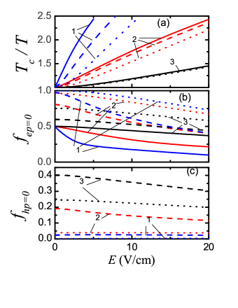
Figure 1: (Color online) Effective temperature $T_{c}/T$ (a) and maximal distribution of electrons $f_{ep=0}$ (b) and holes $f_{hp=0}$ (c) versus electric field for $T=$77 K (1), 150 K (2), and 300 K (3). Solid, dashed, and dotted curves correspond to $V_{g}=$0 V, 1 V, and 3 V, respectively.

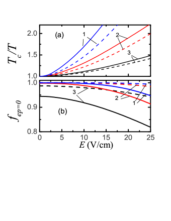
Figure 2: (Color online) Effective temperature $T_{c}/T$ (a) and maximal distribution of electrons $f_{ep=0}$ (b) versus electric field for T =77 K (1), 150 K (2), and 300 K (3). Solid and dashed curves correspond to $V_{g}=$10 V and 20 V, respectively.

In Figs. 1a, 1b, and 1c we plot the effective temperature $T_{c}/T$ and the maximal distributions, $f_{ep=0}$ and $f_{hp=0}$, for different doping levels at $V_{g}$=0 V, 1 V, and 3 V [notice, in Fig. 1(c) the solid curves, pertinent to $V_{g}$=0 V, are omitted as they coincide with the solid curves of Fig. 1b]. It is seen from Fig. 1a that, for given $V_{g}$, the relative increase of the effective temperature of carriers, $T_{c}/T$, with growing $E$ becomes smaller for larger $T$. Fig. 1b shows that the decrease of $f_{ep=0}$ with growing $E$ becomes, at given $T$, slower for larger $V_{g}$. From Figs. 1c and 1b it is seen that $f_{hp=0}$, for given $V_{g}$, quickly decreases as $T$ grows. For heavily doped case, at $V_{g}=$10 V and 20 V, in Figs. 2a and 2b we plot $T_{c}/T$ and $f_{ep=0}$ as functions of $E$. For these gate voltages, the hole concentrations are small, so that $f_{hp=0}<0.1$ and we do not plot the dependencies $f_{hp}$ here. The dependencies $T_{c}/T$ and $f_{ep=0}$ on $T$, $V_{g}$, and $E$ now are similar to those in the low-doping region.

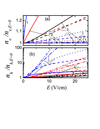
Figure 3: (Color online) Electron (a) and hole (b) concentrations (normalized to their values at $E=0$) versus electric field at $T=$77 K (1), 150 K (2), and 300 K (3). The solid, the dash, the dot, the dash-dot, and the dash-dot-dot curves correspond to $V_{g}=$0 V, 1 V, 3 V, 10 V, and 20 V, respectively.

III.2 Carrier concentrations

Using solutions of the balance Eqs. (12)-(15) in Eq. (3) we plot in Fig. 3a dimensionless concentrations of electrons, $n_{e}/n_{e,E=0}$, and in Fig. 3b of holes, $n_{h}/n_{h,E=0}$. Here $n_{e,E=0}$ and $n_{h,E=0}$ are equilibrium concentration of electrons and holes for $E=0$ and these concentrations are strongly dependent on $V_{g}$ and $T$. 11 For small concentrations (solid and dashed curves in Fig. 3a) of electrons (the main carriers) their concentration is increased on tens of percents for growing $E$. However, for $V_{g}\geq 10$V the concentration of main carriers becomes very weakly growing function of $E$ even at $T=300$K. At the same time, the density of the minor carriers (holes) according to Fig. 3b can be enlarged by tens of times, especially at low temperatures.

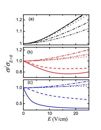
Figure 4: (Color online) Nonlinear conductivity, normalized to its value at $E=0$, versus electric field for: $T=$300 K (a), 150 K (b) and 77 K (c). The solid, the dash, the dot, the dash-dot, and the dash-dot-dot curves correspond to $V_{g}=$ 0 V, 1 V, 3 V, 10 V, and 20 V, respectively.

III.3 Current-voltage characteristics

In Fig. 4, we plot the normalized conductivity $\sigma/\sigma_{E=0}$ versus field $E$ for different levels of doping, dependent on gate voltage varied between $V_{g}=0$ and $V_{g}=$20 V and on different temperatures. Point out $\sigma_{E=0}$ for each curve in Figs. 4 a-c has specific value and $\sigma_{E=0}/\sigma_{0}$ increases essentially when $V_{g}$ grows. 12 The field dependency of the conductivity is determined by a competition between the first and the second terms in Eq. (11). Indeed, as $F_{p=0}$ is a decreasing function of $E$ the integral (second) contribution, for $\mu_{e}l_{c}/\hbar v_{W}\gtrsim 1$ or/and $T_{c}l_{c}/\hbar v_{W}\gtrsim 1$, is either much slower decreasing function of $E$ or even an increasing function of $E$. In particular, for $T_{c}l_{c}/\hbar v_{W}\gtrsim 1$ and $\mu_{e}/T_{c}\gg 1$, the second contribution is the integral of the product of $F_{p}$ (that is $\approx F_{p=0}$ for $\mu_{e}/v_{W}\geq p\geq 0$ and drops rapidly for $p>\mu_{e}/v_{W}$) with the other factor that is a large and growing function of $p$, $\propto p^{2}$, in actual region of $p$, $T_{c}/v_{W}\lesssim p\leq\mu_{e}/v_{W}$. So for low temperatures the contribution $F_{p=0}$ (see Fig. 4 b and c) is essential and leads to the appearance of a minimum in the field dependence of $\sigma$ for small concentrations, for $V_{g}<$ 3V. With the growth of electric field or the concentration (for $V_{g}>$3 V) the main contribution to the conductivity comes from the integral term in Eq. (11) and now $\sigma$ is monotinically growing function of $E$, cf. Fig. 4 a, b, and c. Indeed, pertinent current-voltage characteristics show transition from a sublinear dependence to a superlinear one, as the concentration or/and the temperature grow. For $V_{g}\geq$3 V (and at $T=$300 K for any $V_{g}$, or concentration) a superlinear current-voltage characteristic is realized.

IV Conclusions

In the present work, we investigate the effect of doping on carrier heating in a gated graphene based on the balance equation approach. The effective temperature and concentrations of carriers are studied as functions of the thermostat temperature, the gate voltage, and the applied dc field. Pertinent current-voltage characteristics show the transition from the regime of heating for intrinsic bipolar conductivity to the regime of heating for the conductivity of strongly degenerated carriers. In the latter case the heating is well described by simple analytical formulas, see (16).

Next, we list and discuss the assumptions used in the calculations performed. Here we have examined the heating of carriers in the low energy region only, when the optical phonon emission is not essential and the radiative-induced direct interband transitions are assumed to be the main generation-recombination mechanism. Point out that for much larger electric fields (for $E\gg$0.1 kV/cm, see 2a ) present approach will not be valid as the optical phonon contribution is not taken into account, however, the influence of optical phonons is smaller for a higher level of the doping (gate voltage). We have also restricted ourselves by the study of limiting case when the intercarrier Coulomb scattering is dominating. As shown in 7 for the intrinsic graphene case, this is an adequate approach. Possible contribution of other generation-recombination mechanisms (note, that the Auger-processes are forbidden due to the symmetry of electron-hole states 13 ) require an additional investigation. Further, we have assumed that the heat removal is sufficiently effective (this point becomes insignificant in the case of short electric pulses when the thermostat is not overheated). At last, to describe the momentum relaxation we take into account only the statical disorder scattering using the phenomenological model of Ref. 10 (which is in good agreement with the experimental data; the microscopic mechanisms of scattering are still unclear 14 ). The listed assumptions should not essentially modify the peculiarities of the heating mechanisms, in comparison with a study that will treat relaxation processes in more details; in addition, here many limitations are imposed also because of the lack of data on graphene.

To conclude, essential heating of carriers is shown in present study. It will define different parameters of possible graphene-based devices. In addition, investigation of hot carriers (even within the considered limited region of parameters) gives important information about mechanisms of relaxation and recombination in graphene. Therefore, further experimental and theoretical (including numerical modeling) study of a heating in graphene is very opportunely now.

*

Appendix A Collision integrals

Below we present the collision integrals $J_{qe}$, $J_{r}$ and $J_{cc}$ (deduced in 9 ; 10 and 15 , respectively) that have been used to obtain the balance equations. For quasi-elastic scattering on acoustic phonons the energy relaxation is described by the Fokker-Planck nonlinear differential form

$$J_{qe}\left(f|kp\right)=\frac{\nu_{p}^{(qe)}}{p^{2}}\frac{d}{dp}\left\{p^{4}\left[\frac{df_{kp}}{dp}+\frac{f_{kp}(1-f_{kp})}{p_{T}}\right]\right\}.$$ (17)

Here $k=e,h$ and it is introduced the frequency of quasi-elastic relaxation $\nu_{p}^{(qe)}=v_{qe}p/\hbar$ that contains the characteristic velocity $v_{qe}\propto T$, where for typical parameters of graphene we have $v_{qe}\approx 51.4$ cm/s at $T=300$K. The thermal-radiation-induced interband transitions are being depicted by the collision integrals

$$J_{r}\left(f|p\right)=\nu_{p}^{(r)}\left[N_{2p/p_{T}}(1-f_{ep}-f_{hp})-f_{ep}f_{hp}\right],$$ (18)

that are equal for electrons and holes. In Eq. (18) it is used the frequency of radiative relaxation $\nu_{p}^{(r)}=v_{r}p/\hbar$, where the characteristic velocity $v_{r}\approx 41.6$cm/s for graphene imbedded between SiO₂ substrate and cover layer.

As Auger-processes are forbidden because of the electron-hole symmetry of the bands in graphene 13 , the intercarrier collision integral receives the form

$$J_{cc}\left(f|kp\right)=\sum\limits_{k_{1}=k,k^{\prime}}\int\limits_{0}^{\infty}dp^{\prime}\int\limits_{-\infty}^{\infty}d\Delta pW_{kk_{1}}(pp^{\prime}|\Delta p)$$

$$\times\left[f_{kp+\Delta p}f_{k_{1}p^{\prime}-\Delta p}(1-f_{kp})(1-f_{k_{1}p^{\prime}})\right.$$ (19)

$$\left.-f_{kp}f_{k_{1}p^{\prime}}(1-f_{kp+\Delta p})(1-f_{k_{1}p^{\prime}-\Delta p})\right],$$

where it describes the transitions due to carrier-carrier scattering from the initial states ($k\textbf{p},k^{\prime}\textbf{p}^{\prime}$) to the states ($k\textbf{p}+\Delta\textbf{p},k^{\prime}\textbf{p}^{\prime}-\Delta\textbf{p}$). Here $v_{W}|\Delta\textbf{p}|$ determines transference of the energy for scattering and $k=k^{\prime}$ corresponds to electron-electron or hole-hole transitions whereas the channel $k\neq k^{\prime}$ describes scattering of electrons on holes. Also in Eq. (A) it is carried out average over the angle and as a result the probability of transition $W_{kk^{\prime}}(pp^{\prime}|\Delta p)$ is dependent from $|\textbf{p}|$, $|\textbf{p}^{\prime}|$ and from the transference of the energy $v_{W}\Delta p$. Deduction of the concentration (8) and the energy (9) balance equations, needed, along with Eq. (7), to obtain the parameters of quasiequilibrium distributions Eq. (6), is based on the property of conservation as of the concentration so of the energy density for interparticle scattering as

$$\frac{4}{{L^{2}}}\sum\limits_{\bf p}{J_{cc}\left({f|kp}\right)=0,}~{}~{}~{}\frac{{4v_{W}}}{{L^{2}}}\sum\limits_{\bf p}{pJ_{cc}\left({f|kp}\right)=0.}$$ (20)

These conditions straightforwardly follow from Eq. (A) if take into account the symmetry of the probability of transitions under the interchange of scattering channels $k,\textbf{p}$ and $k^{\prime},\textbf{p}^{\prime}$.

- (1) M. C. Lemme, Solid State Phenomena, 156-158, 499 (2010).
- (2) J. Moser, A. Barreiro, and A. Bachtold, Appl. Phys. Lett. 91, 163513 (2007).
- (3) I. Meric, M. Y. Han, A. F. Yang, B. Ozyilmaz, P. Kim, and K. L. Shepard, Nature Nanotech. 3, 654 (2008); A. Barreiro, M. Lazzeri, J. Moser, F. Mauri, and A. Bachtold, Phys. Rev. Lett. 103, 076601 (2009).
- (4) J. M. Dawlaty, S. Shivaraman, M. Chandrashekhar, F. Rana, and M. G. Spencer Appl. Phys. Lett. 92, 042116 (2008). D. Sun, Z.-K. Wu, C. Divin, X. Li, C. Berger, W. A. de Heer, P. N.First, and T. B. Norris, Phys. Rev. Lett. 101, 157402 (2008). P. A. George, J. Strait, J. Dawlaty, S. Shivaraman, Mvs. Chandrashekhar, F. Rana, and M. G. Spencer, Nanoletters 8, 4248 (2008). R. W. Newson, J. Dean, B. Schmidt, and H. M. van Driel, Opt. Exp. 17, 2326 (2009).
- (5) E. H. Hwang, B.Y.-K. Hu, and S. Das Sarma, Phys. Rev. B 76, 115434 (2007); W.-K. Tse, S. Das Sarma, Phys. Rev. B 79, 235406 (2009); R. Bistritzer and A. H. MacDonald, Phys. Rev. Lett. 102, 206410 (2009).
- (6) A. Akturk and N. Goldsman, J. Appl. Phys. 103, 053702 (2008); R. S. Shishir and D. K. Ferry, J. Phys.: Condens. Matter, 21, 344201 (2009).
- (7) S. Butscher, F. Milde, M. Hirtschulz, E. Malic, and A. Knorr, Appl. Phys. Lett. 91, 203103 (2007); F. Rana, P. A. George, J. H. Strait, J. Dawlaty, S. Shivaraman, Mvs Chandrashekhar, and M. G. Spencer, Phys. Rev. B 79, 115447 (2009); P.N. Romanets and F.T. Vasko, Phys. Rev. B 81, 085421 (2010).
- (8) O.G. Balev, F.T. Vasko, and V. Ryzhii, Phys. Rev. B 79, 165432 (2009).
- (9) E.M. Lifshitz, L.P. Pitaevskii, and V.B. Berestetskii, Quantum Electrodynamics (Butterworth-Heinemann, 1982); P.R. Wallace, Phys. Rev. 71, 622 (1947).
- (10) F.T. Vasko and V. Ryzhii, Phys. Rev. B 76, 233404 (2007).
- (11) A. Satou, F.T. Vasko, and V. Ryzhii, Phys. Rev. B 78, 115431 (2008); F.T. Vasko and V. Ryzhii, Phys. Rev. B 77, 195433 (2008).
- (12) For 0, 1, 3, 10, and 20 V one obtains , , , , and cm-2 at 300 K. The correspondent hole concentrations are , , , , and cm-2, i.e., the number of holes is negligible at 10 V. At 150 and 77 K, essentially lower , are obtaned for V; for V tends to an independent from value and tends to exponentially small value , where is a coefficient.
- (13) For 0, 1, 3, 10, and 20 V one obtains 1.91, 1.97, 2.34, 5.07, and 10.79 at 300 K (Fig. 4a), 1.15, 1.26, 1.73, 4.25V, and 9.57 at 150 K (Fig. 4b), and 1.035, 1.19, 1.65, 4.02, and 9.24 at 77 K (Fig. 4c).
- (14) M.S. Foster and I.L. Aleiner, Phys. Rev. B 79, 085415 (2009).
- (15) L.A. Ponomarenko, R. Yang, T.M. Mohiuddin, M.I. Katsnelson, K.S. Novoselov, S.V. Morozov, A.A. Zhukov, F. Schedin, E.W. Hill, and A. K. Geim, Phys. Rev. Lett. 102, 206603 (2009); S. Adam, P.W. Brouwer, and S. Das Sarma, Phys. Rev. B 79, 201404(R) (2009).
- (16) L. Fritz, J. Schmalian, M. Mueller, and S. Sachdev, Phys. Rev. B 78, 085416 (2008); M. Mueller, L. Fritz, and S. Sachdev, ibid. 78, 115406 (2008).