An Optimal-Time Construction of Euclidean
Sparse Spanners with Tiny Diameter

In STOC’95 [5] Arya et al. showed that for any set of $n$ points in $\mathbb{R}^{d}$, a $(1+\epsilon)$-spanner with diameter at most 2 (respectively, 3) and $O(n\log n)$ edges (resp., $O(n\log\log n)$ edges) can be built in $O(n\log n)$ time. Moreover, it was shown in [5, 27] that for any $k\geq 4$, one can build in $O(n(\log n)2^{k}\alpha_{k}(n))$ time a $(1+\epsilon)$-spanner with diameter at most $2k$ and $O(n2^{k}\alpha_{k}(n))$ edges. The function $\alpha_{k}$ is the inverse of a certain function at the $\lfloor k/2\rfloor$th level of the primitive recursive hierarchy, where $\alpha_{0}(n)=\lceil n/2\rceil,\alpha_{1}(n)=\left\lceil\sqrt{n}\right\rceil,\alpha_{2}(n)=\lceil\log{n}\rceil,\alpha_{3}(n)=\lceil\log\log{n}\rceil,\alpha_{4}(n)=\log^{*}n$, …, etc. It is also known [27] that if one allows quadratic time then these bounds can be improved. Specifically, for any $k\geq 4$, a $(1+\epsilon)$-spanner with diameter at most $k$ and $O(nk\alpha_{k}(n))$ edges can be constructed in $O(n^{2})$ time [27].

A major open problem in this area is whether one can construct within time $O(n\log n+nk\alpha_{k}(n))$ a $(1+\epsilon)$-spanner with diameter at most $k$ and $O(nk\alpha_{k}(n))$ edges. In this paper we answer this question in the affirmative. Moreover, in fact, we provide a stronger result. Specifically, we show that for any $k\geq 4$, a $(1+\epsilon)$-spanner with diameter at most $k$ and $O(n\alpha_{k}(n))$ edges can be built in optimal time $O(n\log n)$. The tradeoff between the diameter and number of edges of our spanners is tight up to constant factors in the entire range of parameters.

1 Introduction

1.1 Euclidean Spanners

Consider a set $S$ of $n$ points in $\mathbb{R}^{d}$ and a number $t\geq 1$. A graph $G=(S,E)$ in which the weight $w(x,y)$ of each edge $e=(x,y)\in E$ is equal to the Euclidean distance $\|x-y\|$ between $x$ and $y$ is called a geometric graph. We say that the graph $G$ is a $t$-spanner for $S$ if for every pair $p,q\in S$ of distinct points, there exists a path in $G$ between $p$ and $q$ whose weight is at most $t$ times the Euclidean distance $\|p-q\|$ between $p$ and $q$. Such a path is called a $t$-spanner path. The problem of constructing Euclidean spanners has been studied intensively over the past two decades [15, 23, 4, 10, 16, 5, 17, 7, 29, 2, 11, 18]. (See also the recent book by Narasimhan and Smid [27], and the references therein.) Euclidean spanners find applications in geometric approximation algorithms, network topology design, geometric distance oracles, distributed systems, design of parallel machines, and other areas [16, 25, 29, 19, 21, 20, 22, 26].

Spanners are important geometric structures, since they enable approximation of the complete Euclidean graph in a much more economical form. First and foremost, a spanner should be sparse, meaning that it can have only a small (ideally, linear) number of edges. However, at the same time, the spanner is required to preserve some fundamental properties of the underlying complete graph. In particular, for some practical applications (e.g., in network routing protocols) it is desirable that the spanner achieves a small diameter, that is, for every pair $p,q\in S$ of distinct points there should be a $t$-spanner path that consists of a small number of edges [6, 1, 2, 11, 18].

In a seminal STOC’95 paper [5], Arya et al. showed that for any set of $n$ points in $\mathbb{R}^{d}$ one can build in $O(n\log n)$ time a $(1+\epsilon)$-spanner with diameter at most 2 and $O(n\log n)$ edges, and another one with diameter at most 3 and $O(n\log\log n)$ edges. Moreover, it was shown in [5, 27] that for any $k\geq 4$, one can build in $O(n(\log n)2^{k}\alpha_{k}(n))$ time a $(1+\epsilon)$-spanner with diameter at most $2k$ and $O(n2^{k}\alpha_{k}(n))$ edges. The function $\alpha_{k}$ is the inverse of a certain function at the $\lfloor k/2\rfloor$th level of the primitive recursive hierarchy, where $\alpha_{0}(n)=\lceil n/2\rceil,\alpha_{1}(n)=\left\lceil\sqrt{n}\right\rceil,\alpha_{2}(n)=\lceil\log{n}\rceil,\alpha_{3}(n)=\lceil\log\log{n}\rceil,\alpha_{4}(n)=\log^{*}n,\alpha_{5}(n)=\lfloor\frac{1}{2}\log^{*}n\rfloor$, $\ldots$, etc. Roughly speaking, for $k\geq 2$ the function $\alpha_{k}$ is close to $\log$ with $\lfloor\frac{k-2}{2}\rfloor$ stars. (See Section 2 for the formal definition of this function.) It is also known [27] that if one allows quadratic time then these bounds can be improved. Specifically, for any $k\geq 4$, a $(1+\epsilon)$-spanner with diameter at most $k$ and $O(nk\alpha_{k}(n))$ edges can be constructed in $O(n^{2})$ time [27].

If one wishes to produce spanners with $o(n\log\log n)$ edges but is willing to spend only $O(n\log n)$ time, then none of the above constructions of [5, 27] is of any help. However, there is another construction of spanners that can be used [11]. Specifically, Chan and Gupta [11] showed that there exists a $(1+{\epsilon})$-spanner with diameter $O(\alpha(m,n))$ and $O(m)$ edges, where $\alpha(\cdot,\cdot)$ is the inverse-Ackermann function. Moreover, the construction of [11] can be implemented in $O(n\log n)$ time. The drawback of this construction, though, is that the constant factor hidden within the $O$-notation of the diameter bound is large. In particular, it does not provide a spanner whose diameter is, say, smaller than 50.

A major open problem in this area is whether one can construct in time $O(n\log n+nk\alpha_{k}(n))$ a $(1+\epsilon)$-spanner with diameter at most $k$ and $O(nk\alpha_{k}(n))$ edges, for any $k\geq 4$. In this paper we answer this question in the affirmative. In fact, we provide a stronger result. Specifically, we show that a $(1+\epsilon)$-spanner with diameter at most $k$ and $O(n\alpha_{k}(n))$ edges can be built in $O(n\log n)$ time.

Note that our tradeoff improves all previous results in a number of senses. In comparison to the construction of [27] that requires a quadratic running time, our construction is (1) drastically faster, and (2) produces a spanner that is sparser by a factor of $k$. In comparison to the result of [5, 27] that for any $k\geq 4$ produces in time $O(n(\log n)2^{k}\alpha_{k}(n))$, a $(1+\epsilon)$-spanner with diameter at most $2k$ and $O(n2^{k}\alpha_{k}(n))$ edges, our construction has (1) a diameter half as large, (2) is faster by a factor of $2^{k}\alpha_{k}(n)$, and (3) produces a spanner that is sparser by a factor of $2^{k}$. Finally, in comparison to the construction of [11], the diameter of our construction is smaller by a significant constant factor. (See Table 1 for a concise comparison of previous and new results.)

	[27]	[5, 27]	[11]	New
Diameter	$k$	$2k$	$O(k)$	$k$
Number of edges	$O(nk\alpha_{k}(n))$	$O(n2^{k}\alpha_{k}(n))$	$O(n\alpha_{k}(n))$	$O(n\alpha_{k}(n))$
Running time	$O(n^{2})$	$O(n(\log n)2^{k}\alpha_{k}(n))$	$O(n\log n)$	$O(n\log n)$

Table 1: A concise comparison of previous and new results on Euclidean spanners. Our results are indicated by bold fonts. It is assumed that $n$ and $k$ are arbitrary parameters, with $k\geq 4$.

There are two particular values of $k$ that deserve special attention. First, for $k=4$ our tradeoff shows that one can build in $O(n\log n)$ time a $(1+\epsilon)$-spanner with diameter at most 4 and $O(n\log^{*}n)$ edges. This result provides the first subquadratic-time construction of $(1+\epsilon)$-spanners with diameter at most $7$ and $o(n\log\log n)$ edges. Second, for $k=2\alpha(n)+2$, our tradeoff gives rise to a diameter at most $2\alpha(n)+2$ and $O(n\alpha_{2\alpha(n)+2}(n))=O(n)$ edges. In all the previous works of [5, 11, 27], a construction of $(1+{\epsilon})$-spanners with diameter $O(\alpha(n))$ and $O(n)$ edges was also provided. However, the constants hidden within the $O$-notation of the diameter bound in the corresponding constructions of [5, 11, 27] are significantly larger than $2$. Since $\alpha(n)\leq 4$ for all practical applications, this improvement on the diameter bound is of practical importance.

Our tradeoff is tight in all respects. Indeed, the upper bound of $O(n\log n)$ on the running time of our construction holds in the algebraic computation-tree model. A matching lower bound is given in [14]. In addition, Chan and Gupta [11] proved that there exists a set of $n$ points on the $x$-axis for which any $(1+\epsilon)$-spanner with at most $m$ edges must have a diameter at least $\alpha(m,n)-4$. This lower bound (cf. Corollary 4.1 therein [11]) implies that our tradeoff of $k$ versus $O(n\alpha_{k}(n))$ between the diameter and number of edges cannot be improved by more than constant factors even for 1-dimensional spaces.

1.2 1-Spanners for Tree Metrics

The tree metric induced by an arbitrary $n$-vertex weighted tree $T$ is denoted by $M_{T}$. A spanning subgraph $G$ of $M_{T}$ is said to be a 1-spanner for $T$, if for every pair of vertices, their distance in $G$ is equal to their distance in $T$. Let $P_{n}$ be the unweighted path graph on $n$ vertices.

In a classical STOC’82 paper [36], Yao showed that there exists a 1-spanner for $P_{n}$ with diameter $O(\alpha(m,n))$ and $O(m)$ edges, for any $m\geq n$. Chazelle [12] extended the result of [36] to arbitrary tree metrics, and presented an $O(m)$-time algorithm for computing a 1-spanner realizing this tradeoff. Thorup [35] provided an alternative algorithmic proof of Chazelle’s result [12], and, in addition, devised an efficient parallel algorithm for computing such a 1-spanner. In all these constructions [36, 12, 35], the constants hidden within the $O$-notation of the diameter bound are significantly larger than 2. In particular, none of these constructions can produce a spanner whose diameter is, say, smaller than 25.

Alon and Schieber [3] and Bodlaender et al. [9] independently showed that a 1-spanner for $P_{n}$ with diameter at most $k$ and $O(n\alpha_{k}(n))$ edges can be built in $O(n\alpha_{k}(n))$ time, for any constant $k\geq 2$. The constructions of [3] and [9] were also extended to arbitrary tree metrics. Specifically, Alon and Schieber [3] showed that for any tree metric, a 1-spanner with diameter at most $2k$ (rather than $k$) and $O(n\alpha_{k}(n))$ edges can be built in $O(n\alpha_{k}(n))$ time. Also, they managed to reduce the diameter bound from $2k$ back to $k$ in the particular cases of $k=2$ and $k=3$. Bodlaender et al. [9] devised a construction of 1-spanners for arbitrary tree metrics with diameter at most $k$ and $O(n\alpha_{k}(n))$ edges. However, the question of whether this construction of Bodlaender et al. can be implemented efficiently was left open in [9], and remained open prior to this work.

Narasimhan and Smid [27] extended the constructions of [3] and [9] to super-constant values of $k$. Specifically, they showed that for any $k\geq 4$ and any tree metric, a 1-spanner with diameter at most $2k$ (respectively, $k$) and $O(n2^{k}\alpha_{k}(n))$ (resp., $O(nk\alpha_{k}(n))$ edges can be built in time $O(n(\log n)2^{k}\alpha_{k}(n))$ (resp., $O(n^{2})$).

On the way to our results for Euclidean spanners, we have improved the constructions of [3, 9, 27] and devised an $O(n\alpha_{k}(n))$-time algorithm that builds 1-spanners for arbitrary tree metrics with diameter at most $k$ and $O(n\alpha_{k}(n))$ edges, for any $k\geq 4$. (See Table 2 for a comparison of previous and new results.)

	Diameter	Number of edges	Running time
[12, 35]	$O(k)$, for any $k$	$O(n\alpha_{k}(n))$	$O(n\alpha_{k}(n))$
[3]	$2k$, for a constant $k\geq 4$	$O(n\alpha_{k}(n))$	$O(n\alpha_{k}(n))$
[27]	$2k$, for any $k\geq 4$	$O(n2^{k}\alpha_{k}(n))$	$O(n(\log n)2^{k}\alpha_{k}(n))$
[9, 27]	$k$, for any $k\geq 4$	$O(nk\alpha_{k}(n))$	$O(n^{2})$
New	$k$, for any $k\geq 4$	$O(n\alpha_{k}(n))$	$O(n\alpha_{k}(n))$
[3]	7	$O(n\log\log n)$	$O(n\log\log n)$
[9, 27]	4	$O(n\log^{*}n)$	$O(n^{2})$
New	$4$	$O(n\log^{*}n)$	$O(n\log^{*}n)$
[12, 35, 3, 27]	$O(\alpha(n))$	$O(n)$	$O(n)$
New	$2\alpha(n)+2$	$O(n)$	$O(n)$

Table 2: A comparison of previous and new results on 1-spanners for arbitrary tree metrics. Our results are indicated by bold fonts.

The running time of our algorithm is linear in the number of edges of the resulting spanners. Also, it was proved in [3] that any 1-spanner for $P_{n}$ with diameter at most $k$ must have at least $\Omega(n\alpha_{k}(n))$ edges. This lower bound implies that the tradeoff between the diameter and number of edges of our spanners is tight in the entire range of parameters.

The problem of constructing 1-spanners for tree metrics is a natural one, and, not surprisingly, has also been studied in more general settings, such as planar metrics [34], general metrics [33], and general graphs [8]. (See also Chapter 12 in [27] for an excellent survey on this problem.) This problem is also closely related to the extremely well-studied problem of computing partial-sums. (See the papers of Tarjan [32], Yao [36], Chazelle and Rosenberg [13],  Pătraşcu and Demaine [28], and the references therein.) For a discussion about the relationship between these two problems see the introduction of [2]. We demonstrate that our construction of 1-spanners for tree metrics is useful for improving key results in the context of Euclidean spanners. We anticipate that this construction would be found useful in the context of partial sums problems, and for other applications such as those discussed in [9, 8]. Finally, we believe that regardless of its applications, this construction is of independent interest.

1.3 Lower Bounds for Euclidean Steiner Spanners

The lower bound of Chan and Gupta [11] on the tradeoff between the diameter and number of edges of Euclidean spanners was mentioned in Section 1.1. Formally, it states that for any ${\epsilon}>0$, there exists a set of $n$ points on the $x$-axis, where $n$ is an arbitrary power of two, for which any $(1+{\epsilon})$-spanner with at most $m$ edges has diameter at least $\alpha(m,n)-4$. Consequently, the corresponding upper bound construction of [11] is optimal up to constant factors. However, the lower bound of Chan and Gupta [11] does not preclude the existence of Euclidean Steiner spanners with diameter $o(\alpha(m,n))$ and $o(m)$ edges.

In this paper we demonstrate that as far as the diameter and number of edges are concerned, Steiner points do not help. Consequently, the upper bound construction of [11], as well as the constructions of Euclidean spanners and spanners for tree metrics that are provided in the current paper, cannot be improved even if one allows the spanner to employ (arbitrarily many) Steiner points.

1.4 Our and Previous Techniques

Arya et al. [5] demonstrated that it is possible to represent Euclidean $(1+\epsilon)$-spanners as a forest $\mathcal{F}$ that consists of a constant number of dumbbell trees, such that for any pair $p,q$ of distinct points, there exists a dumbbell tree $T\in\mathcal{F}$, which satisfies that the path between $p$ and $q$ in $T$ is a $(1+\epsilon)$-spanner path. This remarkable property provides a powerful tool for reducing problems on general graphs to similar problems on trees. Indeed, both constructions of Euclidean sparse spanners with bounded diameter of [5, 27] employ the following four-step scheme. First, build a Euclidean $(1+\epsilon)$-spanner with linear number of edges (and possibly huge diameter) as done, e.g., in [10]. Second, decompose the spanner into a constant number of dumbbell trees as mentioned above. Third, build a sparse 1-spanner with bounded diameter for each of these dumbbell trees. Finally, return the union of these 1-spanners as the ultimate spanner. Chan and Gupta [11] employ a similar approach for building their spanners for doubling metrics. Roughly speaking, instead of working with dumbbell trees, Chan and Gupta use net trees that share similar properties.

Our construction of Euclidean spanners also follows the above four-step scheme. Next, we discuss the technical challenges we faced on the way to achieving an optimal-time construction of 1-spanners for arbitrary $n$-point tree metrics with diameter at most $k$ and $O(n\alpha_{k}(n))$ edges, where $n\geq 0$ and $k\geq 2$ are arbitrary integers.

A central ingredient in the constructions of 1-spanners for tree metrics of [12, 3, 9, 27] is a tree decomposition procedure. Given an $n$-vertex rooted tree $(T,rt)$ and a parameter $\ell$, this procedure computes a set $CV_{\ell}$ of at most $O(n/\ell)$ cut-vertices whose removal from the tree decomposes $T$ into a collection of subtrees of size at most $\ell$ each. For our purposes, it is crucial that the running time of this procedure will be $O(n)$. Equally important, the size of the set $CV_{\ell}$ must not exceed $n/\ell$. None of the decomposition procedures of [12, 3, 9, 27] satisfies these two requirements simultaneously. The decomposition procedure of [27], for example, requires time $O(n\log n)$ rather than $O(n)$, and the size bound of $CV_{\ell}$ is $2(n/\ell)$ rather than $n/\ell$. We remark that the slack of two on the size bound of $CV_{\ell}$ contributes a factor of $2^{k}$ to the number of edges and the running time of the spanner construction of [27]. Also, the slack of $\log n$ on the running time of this procedure contributes an additional factor of $\log n$ to the the running time of the construction of [27]. Consequently, the number of edges and the running time of the spanner construction of [27] are bounded above by $O(n2^{k}\alpha_{k}(n))$ and $O(n(\log n)2^{k}\alpha_{k}(n))$, respectively. The decomposition procedure of [9] is the only one in which the size bound of $CV_{\ell}$ is no greater than $n/\ell$, but it is unclear whether this procedure can be implemented efficiently. In this paper we provide a decomposition procedure that satisfies both these requirements. Our procedure is, in addition, surprisingly simple.

Special attention should be given to determining an optimal value for the parameter $\ell$. In particular, the value of $\ell$ was set to be $\alpha_{k-2}(n)$ in both [3] and [27]. In this paper we define a variant $\alpha^{\prime}_{k}$ of the function $\alpha_{k}$, such that $\alpha_{k}(n)\leq\alpha^{\prime}_{k}(n)\leq 2\alpha_{k}(n)+4$, for all $k,n\geq 0$, and demonstrate that $\alpha^{\prime}_{k-2}(n)$ is a much better choice for $\ell$ than $\alpha_{k-2}(n)$ is. (See Section 2 for the formal definitions of the functions $\alpha_{k}$ and $\alpha^{\prime}_{k}$.) In particular, this optimization enables us to “shave” a factor of $k$ from both the number of edges and the running time of our construction, thus proving that this choice of $\alpha^{\prime}_{k-2}(n)$ for $\ell$ is, in fact, optimal.

Another key ingredient in the constructions of [12, 3, 9, 27] is the computation of an edge set $E^{\prime}$ that connects the cut vertices of $CV_{\ell}$. Alon and Schieber [3] and Narasimhan and Smid [27] employed a natural yet inherently suboptimal approach. First, construct a tree $T^{\prime}$ on the vertex set $CV_{\ell}\cup\{rt\}$ that “inherits” the tree structure of the original tree $(T,rt)$, by making each vertex $u$ of $CV_{\ell}$ a child of the first vertex of $CV_{\ell}\cup\{rt\}$ on the path in $T$ from $u$ to $rt$. Second, recursively compute a sparse 1-spanner for $T^{\prime}$ with diameter at most $k$. Note that every 1-spanner path for $T^{\prime}$ between a pair $u,v$ of vertices, such that $u$ is an ancestor of $v$ in $T^{\prime}$, is also a 1-spanner path for $T$. However, this property does not necessarily hold for a general pair of vertices in $T^{\prime}$, since their least common ancestor might not be in $T^{\prime}$. Consequently, a 1-spanner for $T^{\prime}$ with diameter at most $k$ provides a 1-spanner for $T$ with diameter at most $2k$ rather than $k$. (See Chapter 12 in [27] for further detail.) To overcome this obstacle, Chazelle [12] suggested connecting the vertices of $CV_{\ell}$ into a Steiner tree $\mathcal{T}^{*}$ using as many additional Steiner vertices as needed to guarantee that every 1-spanner path for $\mathcal{T}^{*}$ will also be a 1-spanner path for the original tree $T$. Bodlaender et al. [9] took this idea of [12] one step further and studied a generalized problem of constructing 1-spanners for arbitrary Steiner tree metrics. Specifically, suppose that in $T$, a subset $R(T)\subseteq V(T)$ of the vertices are colored black, and the rest of the vertices in $S(T)=V(T)\setminus R(T)$ are colored white. The black (respectively, white) vertices are called the required vertices (resp., Steiner vertices) of $T$. We say that a 1-spanner $H$ for $T$ has diameter at most $k$ if $H$ contains a 1-spanner path for $T$ that consists of at most $k$ edges, for every pair of required vertices in $T$. Bodlaender et al. [9] provided a construction of 1-spanners for arbitrary Steiner tree metrics with diameter at most $k$ and $O(n\alpha_{k}(n))$ edges, for any constant $k\geq 4$. However, it was unclear prior to this work whether this construction of [9] can be implemented in subquadratic time [27]. In this paper we combine some ideas of [12, 3, 9, 27] with numerous new ideas to produce an algorithm that implements the construction of Bodlaender et al. [9] in optimal-time, and, in addition, extends it to super-constant values of $k$. In particular, we devise a linear time procedure for pruning the redundant vertices of a Steiner tree, while preserving its basic structure and intrinsic properties. Our algorithm makes an extensive use of this pruning procedure, e.g., for pruning the initial Steiner tree from its redundant vertices, and for computing the edge set $E^{\prime}$ that connects the cut vertices of $CV_{\ell}$.

Finally, our extension of the lower bound of [11] to Euclidean Steiner spanners employs a direct combinatorial argument, which shows that any Steiner spanner can be “pruned” from Steiner points, while increasing the number of edges by a small factor and preserving the same diameter. More specifically, we demonstrate that it is possible to replace each edge of the original Steiner spanner with a constant number of edges–none of which is incident on a Steiner point, so that for every pair of required points and any path $P$ in the original Steiner spanner between them, there would be a path $P^{\prime}$ in the resulting graph between these points that consists of the same number of edges as $P$ and whose weight is no greater than that of $P$.

1.5 Structure of the Paper

In Section 2 we present some very slowly growing functions that are used throughout the paper, and analyze their properties. The technical proofs involved in this analysis are relegated to Appendices A and B. Section 3 is devoted to our construction of 1-spanners for tree metrics. Therein we start (Section 3.1) with outlining our basic scheme. We proceed (Section 3.2) with presenting the pruning procedure and providing a few useful properties of the resulting pruned trees. The decomposition procedure is given in Section 3.3. Finally, in Section 3.4 we provide an optimal-time algorithm for computing 1-spanners for tree metrics and analyze its performance. In Section 4 we derive our construction of Euclidean spanners. Our lower bounds for Euclidean Steiner spanners are established in Section 5.

1.6 Definitions and Notation

The size of a tree $T$, denoted $|T|$, is the number of vertices in $T$. The number of edges in a path $P$ is denoted by $|P|$, and the weight of $P$ is denoted by $w(P)$. For a tree $T$ and a subset $C$ of $V(T)$, we denote by $T\setminus C$ the forest obtained from $T$ by removing all vertices in $C$ along with the edges that are incident to them. For a positive integer $n$, we denote the set $\{1,2,\ldots,n\}$ by $[n]$. In what follows all logarithms are in base 2.

2 Some Very Slowly Growing Functions

In this section we present a number of very slowly growing functions that are used throughout.

Following [31, 3, 27], we define the following two very rapidly growing functions $A_{k}$ and $B_{k}$:

• $A_{k}(n)=A_{k-1}(A_{k}(n-1))$, for all $k,n\geq 1$; $A_{0}(n)=2n$, for all $n\geq 0$; $A_{k}(0)=1$, for all $k\geq 1$.

• $B_{k}(n)=B_{k-1}(B_{k}(n-1))$, for all $k,n\geq 1$; $B_{0}(n)=n^{2}$, for all $n\geq 0$; $B_{k}(0)=2$, for all $k\geq 1$.

We define the functional inverses of the functions $A_{k}$ and $B_{k}$ in the following way:

• $\alpha_{2k}(n)=\min\{s\geq 0:A_{k}(s)\geq n\}$, for all $k,n\geq 0$.

• $\alpha_{2k+1}(n)=\min\{s\geq 0:B_{k}(s)\geq n\}$, for all $k,n\geq 0$.

For technical convenience, we define $\log 0=0$. Observe that for all $n\geq 0$: $\alpha_{0}(n)=\lceil n/2\rceil$, $\alpha_{1}(n)=\left\lceil\sqrt{n}\right\rceil$, $\alpha_{2}(n)=\lceil\log{n}\rceil$, $\alpha_{3}(n)=\lceil\log\log{n}\rceil$, $\alpha_{4}(n)=\log^{*}n$, $\alpha_{5}(n)=\lfloor\frac{1}{2}\log^{*}n\rfloor$, …, etc.

The following lemma can be easily verified.

Lemma 2.1

(1) For all $k\geq 0$, the function $\alpha_{k}=\alpha_{k}(n)$ is monotone non-decreasing with $n$.  (2) For all $k\geq 2$ and $n\geq 1$, $\alpha_{k}(n)<n$. Also, for all $n\geq 2$ (respectively, $n\geq 3$), we have $\alpha_{0}(n)<n$ (resp., $\alpha_{1}(n)<n$).  (3) For all $k\geq 0$ and $n\geq 0$, $\alpha_{k+2}(n)\leq\alpha_{k}(n)$.

The following lemma from [27] provides a useful characterization of the function $\alpha_{k}$.

Lemma 2.2 (Lemma 12.1.16 in [27], p. 230)

Let $k\geq 2$ be an arbitrary integer. Then $\alpha_{k}(n)=1+\alpha_{k}(\alpha_{k-2}(n))$, for all $n\geq 3$, and $\alpha_{k}(0)=\alpha_{k}(1)=0$. Also, $\alpha_{k}(2)=0$ if $k$ is odd, and $\alpha_{k}(2)=1$ if $k$ is even.

Next, we define a variant $\alpha^{\prime}_{k}(n)$ of the function $\alpha_{k}$.

• $\alpha^{\prime}_{0}(n)=\alpha_{0}(n)=\lceil n/2\rceil$, for all $n\geq 0$; $\alpha^{\prime}_{1}(n)=\alpha_{1}(n)=\left\lceil\sqrt{n}\right\rceil$, for all $n\geq 0$

• $\alpha^{\prime}_{k}(n)=2+\alpha^{\prime}_{k}(\alpha^{\prime}_{k-2}(n))$, for all $k\geq 2$ and $n\geq k+2$;
  $\alpha^{\prime}_{k}(n)=\alpha_{k}(n)$, for all $k\geq 2$ and $n\leq k+1$.

The following lemma, whose proof appears in Appendix A, is analogous to Lemma 2.1. It establishes key properties of the function $\alpha^{\prime}_{k}$ that will be used in the sequel.

Lemma 2.3

(1) For all $k\geq 2$, the function $\alpha^{\prime}_{k}=\alpha^{\prime}_{k}(n)$ is monotone non-decreasing with $n$.  (2) For all $k\geq 2$ and $n\geq 1$, $\alpha^{\prime}_{k}(n)<n$. Also, for all $n\geq 2$ (respectively, $n\geq 3$), we have $\alpha^{\prime}_{0}(n)<n$ (resp., $\alpha^{\prime}_{1}(n)<n$).  (3) For all $k\geq 2$ and $n\geq 0$, $\alpha^{\prime}_{k+2}(n)\leq\alpha^{\prime}_{k}(n)$.

Observe that for all $k\geq 0$ and $n\geq 0$, $\alpha^{\prime}_{k}(n)\geq\alpha_{k}(n)$. The following lemma, whose proof appears in Appendix B, shows that $\alpha^{\prime}_{k}(n)$ is not much greater than $\alpha_{k}(n)$.

Lemma 2.4

For all $k,n\geq 0$, $\alpha^{\prime}_{k}(n)\leq 2\alpha_{k}(n)+4$.

The Ackermann function is defined by $A(n)=A_{n}(n)$, for all $n\geq 0$, and the one-parameter inverse-Ackermann function is defined by $\alpha(n)=\min\{s\geq 0:A(s)\geq n\}$, for all $n\geq 0$. In [27] it is shown that $\alpha_{2\alpha(n)+2}(n)\leq 4$. (A similar bound was established in [24].) By Lemma 2.4, we get that $\alpha^{\prime}_{2\alpha(n)+2}(n)\leq 12$. Finally, the two-parameter inverse Ackermann function is defined by $\alpha(m,n)=\min\{s\geq 1:A(s,4\lceil m/n\rceil)\geq\log n\}$, for all $m,n\geq 0$.

3 1-Spanners for Tree Metrics

In this section we present our construction of 1-spanners for tree metrics.

3.1 The Basic Scheme

Let $(T,rt)=(V,E,w)$ be an arbitrary $n$-vertex weighted rooted tree, and let $M_{T}$ be the tree metric induced by $T$. Our goal is to compute a sparse 1-spanner for $T$ with bounded diameter. Clearly, $T$ is already a sparse 1-spanner for itself, but its diameter may be huge. We would like to reduce the diameter of $T$ by adding to it a small number of edges.

For a pair $u,v$ of vertices in $T$, we denote by $P_{T}(u,v)$ the unique path in $T$ between $u$ and $v$. Let $H$ be an arbitrary unweighted graph on the vertex set $V$ of $T$. A path $P$ in $H$ between $u$ and $v$ is called $T$-monotone if it is a sub-path of $P_{T}(u,v)$, i.e., if we write $P_{T}(u,v)=(u=v_{0},v_{1},\ldots,v=v_{t})$, then $P$ can be written as $P=(u=v_{i_{0}},v_{i_{1}},\ldots,v_{i_{q}})$, where $0=i_{0}<i_{1}<\ldots<i_{q}=t$. The $T$-monotone distance between a pair $u,v$ of vertices in $H$ is defined as the minimum number of edges in a $T$-monotone path in $H$ connecting them. The $T$-monotone diameter of $H$, denoted $\Lambda_{T}(H)=\Lambda(H)$, is defined as the maximum $T$-monotone distance between any pair of vertices in $H$. (If $T$ is clear from the context, we may write diameter instead of $T$-monotone diameter.) By the triangle inequality, for any $T$-monotone path in $H$, the corresponding weighted path in $M_{T}$ provides a 1-spanner path for $T$. Hence, $H$ translates into a 1-spanner for $T$ with diameter $\Lambda(H)$, and this holds true regardless of the actual weight function $w$ of $T$. We henceforth restrict attention to unweighted trees in the sequel.

Following [9], we study a generalization of the problem for Steiner trees, where there is a designated subset $R(T)\subseteq V$ of required vertices, and the diameter of a 1-spanner for $T$ is defined as the maximum $T$-monotone distance between any pair of required vertices. The required-size of a Steiner tree is defined as the number of required vertices in it. Also, the remaining vertices in $S(T)=V\setminus R(T)$ are called the Steiner vertices of $T$. If the number of Steiner vertices in $T$ is (much) larger than the number of required vertices, it might be possible to prune some redundant Steiner vertices from $T$ while preserving its basic structure and intrinsic properties. A Steiner rooted tree $(T^{\prime},rt^{\prime})$ is called $T$-monotone preserving, if (1) $R(T^{\prime})=R(T)$, and (2) for every pair $u,v$ of required vertices, the unique path $P_{T^{\prime}}(u,v)$ between $u$ and $v$ in $T^{\prime}$ is $T$-monotone. Consider a $T$-monotone preserving tree $(T^{\prime},rt^{\prime})$, and let $u,v$ be an arbitrary pair of required vertices. Note that any $T^{\prime}$-monotone path between $u$ and $v$ is also $T$-monotone. Thus any 1-spanner $H^{\prime}$ for $T^{\prime}$ with $T^{\prime}$-monotone diameter $k$ is also a 1-spanner for $T$ with $T$-monotone diameter $k$.

Our algorithm for constructing 1-spanners for Steiner tree metrics employs the following recursive scheme. We start by pruning the redundant vertices of $T$, thus transforming $T$ into a $T$-monotone preserving tree $T^{\prime}$ that does not contain too many Steiner vertices. We then select a set $CV_{\ell}$ of at most $n/\ell$ cut-vertices whose removal from the tree decomposes it into a collection of subtrees of required-size at most $\ell$ each, for some parameter $\ell$. Next, we would like to connect the cut-vertices using a small number of edges, so that the $T$-monotone distance between any pair of cut-vertices will be small. To this end we (1) compute a copy $\tau$ of $T$ in which the designated set of required vertices is $CV_{\ell}$, (2) prune $\tau$ from its redundant vertices, and (3) call the algorithm recursively on the resulting pruned tree. We then add a small number of edges to connect between cut vertices and subtrees in the spanner. This step is simple and does not involve a recursive call of the algorithm. Finally, we prune each of the subtrees from redundant vertices, and then call the algorithm recursively for each of them.

3.2 The Pruning Procedure

In this section we devise a procedure for pruning the redundant vertices of a Steiner tree while preserving its basic structure. In addition, we provide a few useful properties of pruned trees.

For a Steiner rooted tree $(T,rt)$ and a pair $u,v$ of vertices in $T$, we denote by $LCA_{T}(u,v)$ the least common ancestor (henceforth, LCA) of $u$ and $v$ in $T$. A Steiner vertex $x\in S=S(T)$ in $T$ is called useful if it is the LCA of some pair of required vertices $u,v\in R=R(T)$. Otherwise it is called redundant. We denote by $LCA(T)$ the set of all useful vertices in $T$, i.e., $LCA(T)=\{x\in S~{}|~{}\exists u,v\in R:x=LCA_{T}(u,v)\}$. A Steiner rooted tree with no redundant vertices is called pruned.

We denote the children of the root vertex $rt$ in a Steiner rooted tree $(T,rt)$ by $c_{1},\ldots,c_{ch(rt)}$, where $ch(rt)$ denotes the number of children of $rt$ in $T$. For each index $i\in[ch(rt)]$, let $T_{(i)}$ be the subtree of $T$ rooted at $c_{i}$. We say that the subtree $T_{(i)}$ is required if it contains at least one required vertex, i.e., if $R_{(i)}=R\cap V(T_{(i)})$ is non-empty. Otherwise we say that it is redundant. Notice that all vertices in a redundant subtree are redundant. Denote by $I=I(T)$ the set of all indices $i$, such that $i\in[ch(rt)]$ and $T_{(i)}$ is a required subtree.

Next, we present a linear time procedure $Prune=Prune((T,rt))$ that accepts as input a Steiner rooted tree $(T,rt)$, and transforms it into a pruned $T$-monotone preserving tree $(T^{\prime},rt^{\prime})$.

If $T$ consists of just the single vertex $rt$, then the procedure either leaves $T$ intact if $rt\in R$, or it transforms $T$ into an empty tree if $rt{~{}\not\in~{}}R$. Otherwise, $|T|\geq 2$. For each index $i\in[ch(rt)]$, the tree $(T_{(i)},c_{i})$ is recursively transformed into a pruned $T_{(i)}$-monotone preserving tree $(T^{\prime}_{(i)},c^{\prime}_{i})$. Observe that for each index $i\in[ch(rt)]\setminus I$, $R_{(i)}=\emptyset$ and $T_{(i)}$ is a redundant subtree, and so $T^{\prime}_{(i)}$ is empty. Also, for each index $i\in I$, the subtree $T^{\prime}_{(i)}$ is non-empty. The procedure removes all $[ch(rt)]$ edges connecting the root vertex $rt$ of $T$ with its children. The execution of the procedure then splits into four cases.
Case 1: $rt\in R$. The root vertex $rt$ of $T$ remains the root vertex of $T^{\prime}$, and for each index $i\in[I]$, an edge connecting $rt$ with the root $c^{\prime}_{i}$ of $T^{\prime}_{(i)}$ is added.
Case 2: $rt{~{}\not\in~{}}R$ and $I=\emptyset$. Hence, $R=\emptyset$, and the procedure transforms $T$ into an empty tree.
Case 3: $rt{~{}\not\in~{}}R$ and $|I|=1$. In this case $rt$ is redundant, and there is a single non-empty subtree $T^{\prime}_{(p)}$, i.e., $I=\{p\}$, for some index $p\in[ch(rt)]$. Hence, the procedure removes $rt$ and sets $T^{\prime}=T^{\prime}_{(p)}$.
Case 4: $rt{~{}\not\in~{}}R$ and $|I|\geq 2$. In this case $rt$ is useful. As in case 1, the root $rt$ of $T$ remains the root vertex of $T^{\prime}$, and for each index $i\in[I]$, an edge connecting $rt$ with the root $c^{\prime}_{i}$ of $T^{\prime}_{(i)}$ is added.
(See Figure 1 for an illustration.)

Figure 1: A rooted Steiner tree $(T,rt)$ is depicted on the left, having 8 required vertices $r_{1},\ldots,r_{8}$ and 16 Steiner vertices $rt=s_{1},\ldots,s_{16}$. The two subtrees $T_{(3)}$ and $T_{(5)}$ of $T$ that are depicted within dashed lines are redundant, whereas the other three subtrees $T_{(1)},T_{(2)}$, and $T_{(4)}$ of $T$ are required. The pruned $T$-monotone preserving tree $(T^{\prime},rt^{\prime})$ that is depicted on the right is obtained as a result of the invocation of the procedure $Prune$ on $T$.

It is easy to verify that the procedure $Prune$ can be implemented in linear time.

Next, we analyze the properties of the resulting tree $T^{\prime}$.

The following lemma follows easily from the description of the procedure.

Lemma 3.1

$(T^{\prime},rt^{\prime})$ is a Steiner rooted tree over $V(T^{\prime})=R(T)\cup LCA(T)$, and $R(T^{\prime})=R(T)$. Also, for each index $i\in I$, $(T^{\prime}_{(i)},c^{\prime}_{i})$ is a Steiner rooted tree over $V(T^{\prime}_{(i)})=R(T_{(i)})\cup LCA(T_{(i)})$, and $R(T^{\prime}_{(i)})=R(T_{(i)})$.

Lemma 3.2

For any pair $u,v$ of vertices in $T^{\prime}$, $u$ is an ancestor of $v$ in $T^{\prime}$ iff it is its ancestor in $T$.

Proof:  The proof is by induction on $n^{\prime}=|T^{\prime}|$. The basis $n^{\prime}\leq 1$ holds vacuously.
Induction Step: We assume the correctness of the statement for all smaller values of $n^{\prime}$, $n^{\prime}\geq 2$, and prove it for $n^{\prime}$. Since $n^{\prime}\geq 2$, it must hold that $|I|\geq 1$. Next, we prove the “only if” part. The argument for the “if” part is similar. Consider an arbitrary pair $u,v$ of vertices in $T^{\prime}$, such that $u$ is an ancestor of $v$ in $T^{\prime}$. Next, we show that $u$ is also an ancestor of $v$ in $T$. By Lemma 3.1, for each index $i\in I$, $V(T^{\prime}_{(i)})\subseteq V(T_{(i)})$. The analysis splits into two cases.
Case 1: $|I|=1$ and $rt{~{}\not\in~{}}R$. In this case $T^{\prime}=T^{\prime}_{(p)}$, with $I=\{p\}$. Notice that $u$ and $v$ belong to $T_{(p)}$. By the induction hypothesis for $T^{\prime}_{(p)}$, $u$ is an ancestor of $v$ in $T_{(p)}$, and thus also in $T$.
Case 2: Either $rt\in R$ or $|I|\geq 2$. In both cases $rt(T^{\prime})=rt$, and for each index $i\in I$, the root $c^{\prime}_{i}$ of the subtree $T^{\prime}_{(i)}$ is a child of $rt$ in $T^{\prime}$.
If both $u$ and $v$ belong to the same subtree $T^{\prime}_{(i)}$, for some index $i\in I$, then they both belong to $T_{(i)}$. Hence, by the induction hypothesis for $T^{\prime}_{(i)}$, $u$ is an ancestor of $v$ in $T_{(i)}$, and thus also in $T$.
Since $u$ is an ancestor of $v$ in $T^{\prime}$, $u$ and $v$ cannot belong to different subtrees $T^{\prime}_{(j)}$ and $T^{\prime}_{(k)}$ of $T^{\prime}$, $j,k\in I$. Hence, the remaining case is that $u=rt(T^{\prime})=rt$. Clearly, $rt$ is an ancestor of $v$ in $T$, and we are done.    

Lemma 3.3

For any pair $u,v$ of required vertices, $LCA_{T^{\prime}}(u,v)=LCA_{T}(u,v)$.

Proof:  Write $l^{\prime}=LCA_{T^{\prime}}(u,v)$ and $l=LCA_{T}(u,v)$. First, notice that $l$ is either a required vertex or a useful vertex. By Lemma 3.1, we get that $l$ belongs to $T^{\prime}$. By definition, $l^{\prime}$ is the LCA of $u$ and $v$ in $T^{\prime}$. By Lemma 3.2, it follows that $l^{\prime}$ is a common ancestor of $u$ and $v$ in $T$, and so it must be an ancestor of their LCA $l$ in $T$. Lemma 3.2 implies that $l^{\prime}$ is an ancestor of $l$ also in $T^{\prime}$. However, by applying Lemma 3.2 again, we get that $l$ is a common ancestor of $u$ and $v$ in $T^{\prime}$, and so it must be an ancestor of their LCA $l^{\prime}$ in $T^{\prime}$. It follows that $l^{\prime}=l$.    

Lemmas 3.1 and 3.3 yield the following corollary.

Corollary 3.4

$(T^{\prime},rt^{\prime})$ is pruned.

Proof:  We argue that $LCA(T^{\prime})=LCA(T)$. Indeed, by Lemma 3.1, $V(T^{\prime})=R(T)\cup LCA(T)$ and $R(T^{\prime})=R(T)$. Hence, $S(T^{\prime})=LCA(T)$, and so $LCA(T^{\prime})\subseteq S(T^{\prime})=LCA(T)$. To see why $LCA(T)\subseteq LCA(T^{\prime})$ holds true as well, consider a vertex $l\in LCA(T)$. By definition, $l{~{}\not\in~{}}R(T)$, and there exists a pair of required vertices $u,v\in R(T)$, such that $l=LCA_{T}(u,v)$. Hence, $l{~{}\not\in~{}}R(T^{\prime})$, and by Lemma 3.3, $l=LCA_{T^{\prime}}(u,v)$. It follows that $l\in LCA(T^{\prime})$.

Consequently, $V(T^{\prime})=R(T^{\prime})\cup LCA(T^{\prime})$, and so there are no redundant vertices in $T^{\prime}$.     

Lemma 3.5

For any pair $u,v$ of vertices in $T^{\prime}$, such that $u$ is an ancestor of $v$ in $T^{\prime}$, $P_{T^{\prime}}(u,v)$ is $T$-monotone.

Proof:  Write $P_{T^{\prime}}(u,v)=(u=v_{0},v_{1},\ldots,v=v_{q})$. By Lemma 3.2, for each index $i\in[q]$, $v_{i-1}$ is an ancestor of $v_{i}$ in $T$. Hence, $P_{T^{\prime}}(u,v)$ is a sub-path of $P_{T}(u,v)$, i.e., it is $T$-monotone.     

We conclude that $T^{\prime}$ is $T$-monotone preserving.

Corollary 3.6

For any pair $u,v$ of required vertices, $P_{T^{\prime}}(u,v)$ is $T$-monotone.

Proof:  If $u$ is either an ancestor or a descendant of $v$ in $T^{\prime}$, then the statement follows from Lemma 3.5.

We may henceforth assume that $LCA_{T^{\prime}}(u,v)\neq u,v$. Write $l^{\prime}=LCA_{T^{\prime}}(u,v)$ and $l=LCA_{T}(u,v)$. By Lemma 3.3, $l^{\prime}=l$. Observe that $P_{T^{\prime}}(u,v)$ is a concatenation of the two paths $P_{T^{\prime}}(u,l)$ and $P_{T^{\prime}}(l,v)$, i.e., $P_{T^{\prime}}(u,v)=P_{T^{\prime}}(u,l)\circ P_{T^{\prime}}(l,v)$. Similarly, we have $P_{T}(u,v)=P_{T}(u,l)\circ P_{T}(l,v)$. Lemma 3.5 implies that both $P_{T^{\prime}}(u,l)$ and $P_{T^{\prime}}(l,v)$ are $T$-monotone, or equivalently, $P_{T^{\prime}}(u,l)$ is a sub-path of $P_{T}(u,l)$ and $P_{T^{\prime}}(l,v)$ is a sub-path of $P_{T}(l,v)$. It follows that $P_{T^{\prime}}(u,v)=P_{T^{\prime}}(u,l)\circ P_{T^{\prime}}(l,v)$ is a sub-path of $P_{T}(u,v)=P_{T}(u,l)\circ P_{T}(l,v)$, i.e., $P_{T^{\prime}}(u,v)$ is $T$-monotone.     

Having proved that $T^{\prime}$ is a pruned $T$-monotone preserving tree, we now turn to establish a number of basic properties of pruned trees that will be of use in the sequel.

A Steiner tree in which the number of Steiner vertices is smaller than the number of required vertices is called compact. Note that in any (non-empty) pruned tree $T$, $R\neq\emptyset$ and $S=LCA(T)$. The next lemma implies that any non-empty pruned tree is compact.

Lemma 3.7

For any Steiner rooted tree $(T,rt)$ (not necessarily pruned), $|LCA(T)|\leq\max\{0,|R|-1\}$.

Proof:  The proof is by induction on $n=|T|$. The basis $n=0$ is trivial.
Induction Step: We assume the correctness of the statement for all smaller values of $n$, $n\geq 1$, and prove it for $n$. If $R=\emptyset$, then by definition $LCA(T)=\emptyset$ as well, and we are done.
We henceforth assume that $R$ is non-empty, and so $\max\{0,|R|-1\}=|R|-1$. By definition, for each index $i\in I$, $R_{(i)}\neq\emptyset$, and for each index $i\in[ch(rt)]\setminus I$, $R_{(i)}=\emptyset$. Hence, by the induction hypothesis, for each index $i\in I$, $|LCA(T_{(i)})|\leq\max\{0,|R_{(i)}|-1\}=|R_{(i)}|-1$, and for each index $i\in[ch(rt)]\setminus I$, $LCA(T_{(i)})=\emptyset$. Clearly, the sets $\{R_{(i)}\}_{i\in I}$ and $\{LCA(T_{(i)})\}_{i\in I}$ are pairwise disjoint. The analysis splits into three cases.
Case 1: $rt\in R$. In this case $R=\bigcup_{i\in I}R_{(i)}\cup\{rt\}$ and $LCA(T)=\bigcup_{i\in I}LCA(T_{(i)})$, implying that $|R|=\sum_{i\in I}|R_{(i)}|+1$ and $|LCA(T)|=\sum_{i\in I}|LCA(T_{(i)})|$. Altogether,

$$|LCA(T)| = \sum_{i\in I}|LCA(T_{(i)})|~{}\leq~{}\sum_{i\in I}\left(|R_{(i)}|-1\right)~{}=~{}\sum_{i\in I}|R_{(i)}|-|I|~{}\leq~{}\sum_{i=1}|R_{(i)}|~{}=~{}|R|-1.$$

Case 2: $rt$ is redundant, i.e., $rt\in S\setminus LCA(T)$. Since $R\neq\emptyset$ and $rt$ is redundant, it must hold that $|I|=1$, i.e., $I=\{p\}$, for some index $p\in[ch(rt)]$. Hence, $R=R_{(p)}$ and $LCA(T)=LCA(T_{(p)})$, implying that $|LCA(T)|~{}=~{}|LCA(T_{(p)})|~{}\leq~{}|R_{(p)}|-1~{}=~{}|R|-1.$
Case 3: $rt$ is useful, i.e., $rt\in LCA(T)$. In this case there must be at least two different required subtrees $T_{(j)}$ and $T_{(k)}$, $j,k\in I$, and so $|I|\geq 2$. Observe that $R=\bigcup_{i\in I}R_{(i)}$ and $LCA(T)=\bigcup_{i\in I}LCA(T_{(i)})\cup\{rt\}$, implying that $|R|=\sum_{i\in I}|R_{(i)}|$ and $|LCA(T)|=\sum_{i\in I}|LCA(T_{(i)})|+1$. It follows that

$$|LCA(T)| = \sum_{i\in I}|LCA(T_{(i)})|+1~{}\leq~{}\sum_{i\in I}\left(|R_{(i)}|-1\right)+1~{}=~{}\sum_{i\in I}|R_{(i)}|-|I|+1$$

$$\leq \sum_{i\in I}|R_{(i)}|-1~{}=~{}|R|-1.$$

   

Lemma 3.8

For a non-empty pruned tree $(T,rt)$, its depth $h(T)$ is at most $|R|-1$ and its diameter $\Lambda(T)$ is at most $|R|$. Moreover, $\Lambda(T)$ is equal to $|R|$ only if the following conditions hold: (1) $rt{~{}\not\in~{}}R$,  (2) $rt$ has exactly two children, and  (3) For any pair $u,v$ of vertices in $T$ for which $|P_{T}(u,v)|=|R|$, $u,v\neq rt=LCA_{T}(u,v)$.

Proof:  The proof is by induction on $n=|T|$. The basis $n=1$ is trivial.
Induction Step: We assume the correctness of the statement for all smaller values of $n$, $n\geq 2$, and prove it for $n$. Since $T$ is pruned, all the subtrees $T_{(1)},\ldots,T_{(ch(rt))}$ of $T$ are pruned as well, and so the induction hypothesis applies to every one of them.

Fix an arbitrary index $i\in[ch(rt)]$. Since $T_{(i)}$ is pruned, we have $|R_{(i)}|\geq 1$. We argue that $|R_{(i)}|\leq|R|-1$. This is clearly the case if $rt\in R$. Otherwise, $rt$ must be useful, and so it must have at least two children in $T$. Hence, there is another index $j\in[ch(rt)]$, such that $|R_{(j)}|\geq 1$. Since $R_{(i)}\cup R_{(j)}\subseteq R$, we get that $|R_{(i)}|\leq|R|-|R_{(j)}|\leq|R|-1$.

By the induction hypothesis, for each index $i\in[ch(rt)]$, $h(T_{(i)})\leq|R_{(i)}|-1\leq|R|-2$. Hence,

$$h(T)~{}=~{}\max\{h(T_{(i)})~{}|~{}i\in[ch(rt)]\}+1~{}\leq~{}|R|-2+1=|R|-1.$$

To bound the diameter $\Lambda(T)$ of $T$, consider a pair $u,v$ of vertices in $T$ for which $|P_{T}(u,v)|=\Lambda(T)$. If $u$ and $v$ belong to the same subtree $T_{(i)}$ of $T$, for some index $i\in[ch(rt)]$, then $\Lambda(T)=\Lambda(T_{(i)})$, and by the induction hypothesis for $T_{(i)}$, we get that $\Lambda(T)=\Lambda(T_{(i)})\leq|R_{(i)}|\leq|R|-1$. Otherwise, $rt=LCA_{T}(u,v)$. If either $u$ or $v$ is the root vertex $rt$, then $\Lambda(T)\leq h(T)\leq|R|-1$.
So far we have proved that in order to obtain $\Lambda(T)\geq|R|$, it must hold that $u,v\neq rt=LCA_{T}(u,v)$. We may henceforth assume that $u,v\neq rt=LCA_{T}(u,v)$. In other words, $u$ and $v$ belong to different subtrees $T_{(i)}$ and $T_{(j)}$ of $T$, respectively, for some indices $i,j\in[ch(rt)]$. Observe that $|P_{T}(u,v)|\leq h(T_{(i)})+h(T_{(i)})+2$. By the induction hypothesis for $T_{(i)}$ and $T_{(j)}$, $h(T_{(i)})\leq|R_{(i)}|-1$ and $h(T_{(j)})\leq|R_{(j)}|-1$, and so $|P_{T}(u,v)|\leq|R_{(i)}|+|R_{(j)}|$. It follows that $\Lambda(T)=|P_{T}(u,v)|\leq|R_{(i)}|+|R_{(j)}|\leq|R|$. Moreover, one can have $\Lambda(T)=|R|$ only if $|R_{(i)}|+|R_{(j)}|=|R|$, in which case both $rt{~{}\not\in~{}}R$ and $ch(rt)=2$ must hold.     

Corollary 3.9

Let $(T,rt)$ be a pruned tree, such that $rt$ has exactly two children $c_{1}$ and $c_{2}$, and let $\tilde{T}$ be the graph obtained from $T$ by adding to it the edge $(c_{1},c_{2})$. Then the $T$-monotone diameter $\Lambda(\tilde{T})$ of $\tilde{T}$ is at most $|R|-1$.

Proof:  Consider a pair $u,v$ of vertices in $\tilde{T}$ for which their $T$-monotone distance $\delta$ satisfies $\Lambda(\tilde{T})=\delta$. Since $\tilde{T}$ contains all edges of $T$, we have $\delta\leq|P_{T}(u,v)|$. If $|P_{T}(u,v)|\leq|R|-1$, then we are done. Otherwise, by Lemma 3.8, $|P_{T}(u,v)|=|R|$ and $u,v\neq rt=LCA_{T}(u,v)$. Hence, either $u$ belongs to $T_{(1)}$ and $v$ belongs to $T_{(2)}$, or vice versa. Suppose without loss of generality that $u$ belongs to $T_{(1)}$ and $v$ belongs to $T_{(2)}$, and write $P_{T}(u,v)=(u=v_{0},v_{1},\ldots,c_{1}=v_{j-1},rt=v_{j},c_{2}=v_{j+1},v_{j+2},\ldots,v=v_{|R|})$. Notice that $\tilde{T}$ contains all edges of $P_{T}(u,v)$, and, in addition, the edge $(c_{1},c_{2})$, which can be used as a shortcut to avoid the detour $(c_{1},rt,c_{2})$ around $rt$. Hence, $\tilde{T}$ contains the $T$-monotone path $\tilde{P}=(u=v_{0},v_{1},\ldots,c_{1}=v_{j-1},c_{2}=v_{j+1},v_{j+2},\ldots,v=v_{|R|})$ that consists of $|R|-1$ edges, and so $\Lambda(\tilde{T})=\delta\leq|\tilde{P}|=|R|-1$.     

3.3 Tree Decomposition Procedure

In this section we devise a procedure $Decomp$ for decomposing a Steiner tree into subtrees in an optimal way.

Let $n$ be an arbitrary positive integer. The procedure $Decomp=Decomp((T,rt),\ell)$ accepts as input a Steiner rooted tree $(T,rt)$ with required-size $n$ and a positive integer $\ell$, and returns as output a set $CV_{\ell}\subseteq V(T)$ of cut vertices. We do not require that a cut vertex would belong to $R=R(T)$.

For each vertex $v$ in $T$ we hold a variable $size(v)$. Also, we initialize the set $CV_{\ell}$ to $\emptyset$. The procedure visits the vertices of $T$ in a post-order manner, so that a vertex $v$ is visited only after all its children have been visited. For each visited vertex $v$, the procedure assigns $size(v)=1+\sum_{u\in Ch(v)}size(u)$ if $v\in R$, and $size(v)=\sum_{u\in Ch(v)}size(u)$ otherwise, where $Ch(v)$ denotes the set of children of $v$ in (the current tree) $T$. (If $v$ is a leaf, then $Ch(v)=NULL$, and so $size(v)=1$ if $v\in R$, and $size(v)=0$ otherwise.) Also, if $size(v)>\ell$, the procedure designates $v$ as a cut vertex by inserting it to $CV_{\ell}$, and then removes the subtree $T_{v}$ of $T$ rooted at $v$ from $T$. (See Figure 2 for an illustration.)

Figure 2: An illustration of a rooted Steiner tree $(T,rt)$ over the vertices $v_{1},v_{2},\ldots,v_{26}$, where $rt=v_{26}$, and for each $i\in[26]$, $v_{i}$ is the $i$th visited vertex in a (left-to-right) post-order traversal. Each vertex $v_{i}$ in the tree is represented as a two-cell rectangle, with the left cell holding its name $v_{i}$, and the right one holding the value of $size(v_{i})$. The 15 required vertices of the tree are depicted within solid lines, whereas the 11 Steiner vertices are depicted within dashed lines. The three vertices whose bounding rectangles are filled, i.e., $v_{7},v_{16}$ and $v_{20}$, comprise the set $CV_{3}$ of cut-vertices that is returned as output of the call $Decomp((T,rt),\ell=3)$.

First, notice that the running time of the procedure $Decomp$ is linear in the number of vertices in $T$. In particular, if $T$ is pruned, then the running time of this procedure is $O(n)$.

We proceed by making the following observation.

Observation 3.10

At the end of the execution of the procedure $Decomp$, for any subtree $\tau\in T\setminus CV_{\ell}$ and any vertex $w\in\tau$, $size(w)$ holds the required-size of the subtree $\tau_{w}$ of $\tau$ rooted at $w$, i.e., $size(w)=|R(\tau_{w})|$.

Next, we obtain upper bounds on the maximum required-size of a subtree in $T\setminus CV_{\ell}$ and the size of the set $CV_{\ell}$ of cut vertices that is returned by the procedure $Decomp$.

Lemma 3.11

(1) The required-size $|R(\tau)|$ of any subtree $\tau\in T\setminus CV_{\ell}$ is at most $\ell$. (2) $|CV_{\ell}|\leq\lfloor\frac{n}{\ell+1}\rfloor$.

Proof:  (1) Consider an arbitrary subtree $\tau\in T\setminus CV_{\ell}$, and let $x$ be the root vertex of $\tau$. By the description of the procedure and Observation 3.10, we have $|R(\tau)|=|R(\tau_{x})|=size(x)\leq\ell$, as otherwise $x$ would have been designated as a cut vertex.
(2) Immediately after a cut vertex $v$ is inserted into $CV_{\ell}$, the procedure removes the subtree $T_{v}$ of $T$ rooted at $v$ from $T$, and so the required-size of the tree $T$ is being decreased by $|R(T_{v})|$ units. Define $\chi(v)=1$ if $v\in R$, and $\chi(v)=0$ otherwise. By the description of the procedure and Observation 3.10, just before the removal of $T_{v}$ from $T$ we have

$$|R(T_{v})|~{}=~{}\chi(v)+\sum_{u\in Ch(v)}|R(T_{u})|~{}=~{}\chi(v)+\sum_{u\in Ch(v)}size(u)~{}=~{}size(v)~{}>~{}\ell,$$

implying that the required-size of $T$ is being decreased by at least $\ell+1$ units. Hence, after $i$ cut vertices have been inserted into $CV_{\ell}$, the required size of $T$ is at most $n-i(\ell+1)$. Also, from the moment the required-size of $T$ becomes at most $\ell$, the set $CV_{\ell}$ remains intact, and we are done.     

Remark: The tradeoff $\ell$ versus $\lfloor\frac{n}{\ell+1}\rfloor$ between the required-size of a subtree in $T\setminus CV_{\ell}$ and the size of the set $CV_{\ell}$ of cut-vertices is tight, and is realized when $T$ is the unweighted path graph $P_{n}$.

3.4 Sparse 1-Spanners for Tree Metrics with Bounded Diameter

In this section we present an optimal time construction of sparse 1-spanners for Steiner tree metrics with bounded diameter. Our spanners achieve a tight tradeoff between the diameter and number of edges.

Let $(T,rt)$ be a Steiner rooted tree. Notice that $T$ can be transformed in linear time into a pruned $T$-monotone preserving tree $(T^{\prime},rt^{\prime})$ by invoking the procedure $Prune$ described in Section 3.2 on $T$. Also, any 1-spanner for $T^{\prime}$ provides a 1-spanner for the original tree $T$ with the same diameter. We may henceforth assume that the original tree $T$ is pruned, i.e., $T=T^{\prime}$. We also assume that for each vertex $v$ in $T$, it can be decided in constant time whether it is black or white, i.e., whether $v\in R(T)$ or $v\in S(T)$.

Next, we describe an algorithm $Tree1Spanner=Tree1Spanner((T,rt),n,k)$ that accepts as input a pruned tree $(T,rt)$, an integer $n\geq 0$ that designates the required-size of $T$, and an integer $k\geq 2$, and returns as output a 1-spanner for $T$.

If $0\leq n\leq k$, return the edge set $E(T)$ of $T$.

If $n=k+1$, check whether $rt$ has exactly two children. If this is the case, return $E(T)\cup\{(c_{1},c_{2})\}$, where $c_{1}$ and $c_{2}$ designate the two children of $rt$. Otherwise, return $E(T)$.

We henceforth assume that $n\geq k+2$. The execution of the algorithm splits into six steps.

At the first step, set $\ell=\alpha^{\prime}_{k-2}(n)$, and compute the set $CV_{\ell}$ of cut vertices of $T$ by making the call $Decomp((T,rt),\ell)$.

At the second step, compute the edge set $E^{\prime}$ that connect the cut vertices.
If $k=2$, set $E^{\prime}=\emptyset$. If $k=3$, set $E^{\prime}$ as the edge set of the complete graph over $CV_{\ell}$.
For $k\geq 4$, proceed in the following way. First, compute a copy $\tau$ of $T$. Second, go over all the vertices of $\tau$ and color the vertices of $CV_{\ell}$ in black, and the remaining vertices in white. (Thus $R(\tau)=CV_{\ell}$, and $S(\tau)=V(T)\setminus CV_{\ell}$.) Third, compute the pruning $\tau^{\prime}$ of $\tau$ by making the call $Prune((\tau,rt))$. Fourth, set $E^{\prime}$ as the edge set returned by the recursive call $Tree1Spanner((\tau^{\prime},rt(\tau^{\prime})),|CV_{\ell}|,k-2)$.

At the third step, compute the subtrees $T_{1},\ldots,T_{g}$ in $T\setminus CV_{\ell}$.

At the fourth step, compute the edge set $E^{\prime\prime}$ that connects the cut vertices of $CV_{\ell}$ with the corresponding subtrees. Specifically, the set of all cut vertices $u\in CV_{\ell}$ that are connected by an edge of $T$ to some vertex of $T_{i}$ is called the border of $T_{i}$, for each $i\in[g]$. The vertex $u$ is called a border vertex of $T_{i}$. Compute the edge set $E^{\prime\prime}=\{(u,v)~{}|~{}v\in R(T)\setminus CV_{\ell},u\in CV_{\ell},u\mbox{ is a border vertex of the subtree to which }v\mbox{ belongs}\}.$
(See Figure 3 for an illustration.)

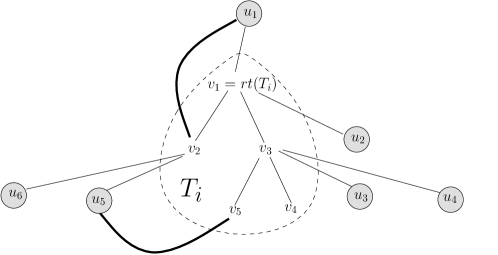
Figure 3: An illustration of a subtree $T_{i}\in T\setminus CV_{\ell}$ that contains the five vertices $rt=v_{1},v_{2},\ldots,v_{5}$, with $v_{3}$ being the only Steiner vertex in $T_{i}$. The border of $T_{i}$ is comprised of the six vertices $u_{1},u_{2},\ldots,u_{6}$ that are depicted within filled circles. Each required vertex $v_{j}$ in $T_{i}$, $j\in[5],j\neq 3$, is incident on the single upstream edge $(u_{1},v_{j})$, and on the five downstream edges $(u_{2},v_{j}),(u_{3},v_{j}),(u_{4},v_{j}),(u_{5},v_{j})$ and $(u_{6},v_{j})$. The upstream edge $(u_{1},v_{2})$ and the downstream edge $(u_{5},v_{5})$ are depicted by bold lines.

At the fifth step we would like to proceed recursively for each of the subtrees $T_{1},\ldots,T_{g}$. To this end, first compute the pruning $T^{\prime}_{i}$ of the subtree $T_{i}$, for each $i\in[g]$, by making the call $Prune((T_{i},rt(T_{i}))$. Then, set $E_{i}$ to be the edge set that is returned by the recursive call $Tree1Spanner((T^{\prime}_{i},rt(T^{\prime}_{i})),|R_{i}|,k)$, for each $i\in[g]$, where $R_{i}=R(T_{i})$.

Finally, at the sixth step, return the edge set $E=E^{\prime}\cup E^{\prime\prime}\cup\bigcup_{i=1}^{g}E_{i}$.

The following theorem summarizes the properties of Algorithm $Tree1Spanner((T,rt),n,k)$.

Theorem 3.12

Let $k\geq 2$ and $n\geq 0$ be two arbitrary integers, and let $(T,rt)$ be a pruned tree with required-size $n$. Algorithm $Tree1Spanner((T,rt),n,k)$ computes in time $O(n\alpha_{k}(n))$ a 1-spanner $G_{T}=(V(T),E)$ for $T$, having diameter at most $k$ and $O(n\alpha_{k}(n))$ edges.

Remarks: (1) If we set $\ell=\alpha_{k-2}(n)$ instead of $\ell=\alpha^{\prime}_{k-2}(n)$ at the first step of the algorithm, then both the running time of the algorithm and the number of edges in the resulting spanner $G_{T}$ would increase by a factor of $k$, i.e., from $O(n\alpha_{k}(n))$ to $O(nk\alpha_{k}(n))$.  (2) In Section 2 we saw that $\alpha_{2\alpha(n)+2}(n)\leq 4$. Hence, we can compute in $O(n)$ time a 1-spanner for $T$ having diameter at most $2\alpha(n)+2$ and $O(n)$ edges.

In what follows we prove Theorem 3.12.

The next lemma bounds the size of the edge set $E^{\prime\prime}$ that is computed at the fourth step of the algorithm and the time needed to compute it. This lemma was essentially proved in [9, 27].

Lemma 3.13

The edge set $E^{\prime\prime}$ contains at most $2n$ edges. Also, it can be computed in $O(n)$ time.

Proof:  Every edge of $E^{\prime\prime}$ is incident on exactly one cut vertex. Consider such an edge $(u,v)\in E^{\prime\prime}$, where $u\in CV_{\ell}$ and $v\in R(T)\setminus CV_{\ell}$. Then $v$ belongs to some subtree $T_{i}$ in $T\setminus CV_{\ell}$. We say that the edge $(u,v)$ is upstream if $u$ is the parent of the root $rt(T_{i})$ of the subtree to which $v$ belongs. Otherwise, the edge $(u,v)$ is called downstream. (See Figure 3 for an illustration.)

By definition, each vertex $v\in R\setminus CV_{\ell}$ is incident on at most one upstream edge. Hence, there are at most $|R\setminus CV_{\ell}|\leq|R|=n$ upstream edges in total.
The downstream edges are counted per cut vertex. Each cut vertex $u\in CV_{\ell}\setminus\{rt\}$ has one parent in $T$, denoted $\pi_{T}(u)$. If $\pi_{T}(u)\in CV_{\ell}$, then no downstream edge is incident on $u$. Otherwise, $\pi_{T}(u)$ belongs to some subtree $T_{i}\in T\setminus CV_{\ell}$. Each downstream edge that is incident on $u$ belongs to a distinct required vertex in $T_{i}$. Hence, the first assertion of Lemma 3.11 implies that $u$ is incident on at most $\ell$ downstream edges. By the second assertion of Lemma 3.11, $|CV_{\ell}|\leq\lfloor\frac{n}{\ell+1}\rfloor$. Summing over all vertices in $CV_{\ell}\setminus\{rt\}$, we get a total of at most $\lfloor\frac{n}{\ell+1}\rfloor\ell\leq n$ downstream edges. Hence, there are overall at most $2n$ edges in $E^{\prime\prime}$.

To verify that $E^{\prime\prime}$ can indeed be constructed within $O(n)$ time, we refer to Exercise 12.4 in [27].     

Next, we prove Theorem 3.12 in the particular case of $k=2$.

Lemma 3.14

Let $(T,rt)$ be a pruned tree with required-size $n\geq 0$. Algorithm $Tree1Spanner((T,rt),n,2)$ computes in $O(n\alpha_{2}(n))$ time a 1-spanner $G_{T}=(V(T),E)$ for $T$, having diameter at most 2 and at most $n\alpha_{2}(n)$ edges.

Proof:  We denote by $F_{2}(n)$ the maximum number of edges in the graph computed by Algorithm $Tree1Spanner((T,rt),n,2)$, where $T$ ranges over all pruned trees having required-size $n$. We next prove by induction on $n$ that $F_{2}(n)\leq n\alpha_{2}(n)$. Let $T$ be a pruned tree with required-size $n$ for which the edge set $E$ that is computed by Algorithm $Tree1Spanner((T,rt),n,2)$ has $F_{2}(n)$ edges.
The case $n=0$ is trivial. We henceforth assume that $n\geq 1$.
By Lemma 3.7, any non-empty pruned tree is compact. Hence, $|V(T)|\leq 2|R(T)|-1=2n-1$, and so $|E(T)|=|V(T)|-1\leq 2n-2$.
If $n\leq 2$, then $F_{2}(n)~{}=~{}|E|~{}=~{}|E(T)|~{}\leq~{}2n-2$. If $n=1$, then $\alpha_{2}(n)=0$, yielding $F_{2}(n)\leq 2n-2=0=n\alpha_{2}(n)$. If $n=2$, then $\alpha_{2}(n)=1$, yielding $F_{2}(n)\leq 2n-2=2=n\alpha_{2}(n)$.
Suppose next that $n=3$. In this case the edge set $E$ returned by the algorithm contains at most one more edge in addition to the edge set $E(T)$ of the input tree $T$. Hence, $F_{2}(n)~{}=~{}|E|~{}\leq~{}|E(T)|+1~{}\leq~{}2n-1~{}=~{}5$. Notice that $\alpha_{2}(3)=2$, yielding $F_{2}(n)\leq 5\leq n\alpha_{2}(n)$.
Induction Step: We assume the correctness of the statement for all smaller values of $n$, $n\geq 4$, and prove it for $n$. Note that $\ell=\alpha^{\prime}_{0}(n)=\alpha_{0}(n)=\lceil n/2\rceil$. By the second assertion of Lemma 3.11, $|CV_{\ell}|\leq\left\lfloor\frac{n}{\ell+1}\right\rfloor\leq\left\lfloor\frac{n}{n/2+1}\right\rfloor=1$, implying that $CV_{\ell}$ consists of a single vertex, denoted $w$.
Observe that for $k=2$, the edge set $E^{\prime}$ is empty.
Since $CV_{\ell}$ consists of a single vertex $w$, the edge set $E^{\prime\prime}$ that is computed at the fourth step of the algorithm is comprised of all edges that connect $w$ to the required vertices in $R(T)\setminus\{w\}$. Hence, $|E^{\prime\prime}|=|R(T)\setminus\{w\}|\leq|R(T)|=n$.
Let $i$ be an index in $[g]$, and consider the edge set $E_{i}$ that is computed at the fifth step of the algorithm. We have $|E_{i}|\leq F_{2}(|R_{i}|)$. By the first assertion of Lemma 3.11, the required-size of each subtree in $T\setminus CV_{\ell}=T\setminus\{w\}$ is at most $\ell$, and so $|R_{i}|\leq\ell=\lceil n/2\rceil<n$. Since the function $\alpha_{2}$ is monotone non-decreasing, the induction hypothesis implies that $|E_{i}|\leq|R_{i}|\alpha_{2}(\ell)$. Since $n\geq 4$, we have $\alpha_{2}(n)=1+\alpha_{2}(\alpha_{0}(n))=1+\alpha_{2}(\ell)$. Also, notice that $\sum_{i=1}^{g}|R_{i}|\leq|R|=n$. It follows that

$$\sum_{i=1}^{g}|E_{i}|~{}\leq~{}\sum_{i=1}^{g}|R_{i}|\alpha_{2}(\ell)~{}=~{}\sum_{i=1}^{g}|R_{i}|(\alpha_{2}(n)-1)~{}\leq~{}n(\alpha_{2}(n)-1).$$

Altogether,

$$F_{2}(n)~{}=~{}|E|~{}=~{}|E^{\prime}|+|E^{\prime\prime}|+\sum_{i=1}^{g}|E_{i}|~{}\leq~{}0+n+n(\alpha_{2}(n)-1)~{}=~{}n\alpha_{2}(n).$$

Next, we prove that $G_{T}$ is a 1-spanner for $T$ with diameter at most 2. The proof is, again, by induction on $n$. The case $n\leq 3$ follows from Lemma 3.8 and Corollary 3.9.
Induction Step: We assume the correctness of the statement for all smaller values of $n$, $n\geq 4$, and prove it for $n$. We show that for an arbitrary pair $u,v$ of required vertices, there is a $T$-monotone path in $G_{T}$ that consists of at most two edges. Consider the single vertex $w$ in $CV_{\ell}$. If either $u$ or $v$ is equal to $w$, then $u$ and $v$ are connected by an edge of $E^{\prime\prime}$, and so this edge forms a $T$-monotone path between $u$ and $v$. If $u$ and $v$ are in different subtrees of $T\setminus\{w\}$, then both edges $(u,w)$ and $(w,v)$ belong to $G_{T}$, and so $u$ and $v$ are connected by the path $P=(u,w,v)$ in $G_{T}$. Notice that the unique path $P_{T}(u,v)$ between $u$ and $v$ must traverse $w$, implying that $P$ is $T$-monotone. Finally, if $u$ and $v$ belong to the same subtree $T_{i}$ in $T\setminus\{w\}$, then by the induction hypothesis they are connected by a $T_{i}$-monotone path $P_{i}$ that consists of at most two edges. However, $P_{i}$ is also a path in $G_{T}$, and it is $T$-monotone.

Denote by $C_{2}(n)$ the worst-case running time of Algorithm $Tree1Spanner((T,rt),n,2)$, where $T$ ranges over all pruned trees $T$ with required-size $n$. We next show that $C_{2}(n)=O(n\alpha_{2}(n))$.
Clearly, if $n\leq 3$, then $C_{2}(n)=O(1)$. We may henceforth assume that $n\geq 4$.
Computing the set $CV_{\ell}$ of cut vertices at the first step of the algorithm takes $O(n)$ time. Also, $E^{\prime}=\emptyset$, and so the second step of the algorithm requires only $O(1)$ time. It takes $O(n)$ time to compute the subtrees $T_{1},\ldots,T_{g}$ and the corresponding pruned subtrees $T^{\prime}_{1},\ldots,T^{\prime}_{g}$ at the third and fifth steps of the algorithm, respectively. Recall that $CV_{\ell}$ consists of a single vertex $w$, and so one can compute the edge set $E^{\prime\prime}=\{(w,v)~{}|~{}v\in R(T)\setminus\{w\}\}$ directly within $O(n)$ time as well. Finally, the time needed to compute the edge sets $E_{1},E_{2},\ldots,E_{g}$ at the fifth step of the algorithm is at most $\sum_{i=1}^{g}C_{2}(|R_{i}|)$. We obtain the recurrence $C_{2}(n)=O(n)+\sum_{i=1}^{g}C_{2}(|R_{i}|)$, where $|R_{i}|\leq\ell=\lceil n/2\rceil$, for each index $i\in[g]$, and $\sum_{i=1}^{g}|R_{i}|\leq n$. Hence, as in the above argument for bounding $F_{2}(n)$, it can be shown that $C_{2}(n)=O(n\alpha_{2}(n))$.     

Next, we prove Theorem 3.12 in the particular case of $k=3$.

Lemma 3.15

Let $(T,rt)$ be a pruned tree with required-size $n\geq 0$. Algorithm $Tree1Spanner((T,rt),n,3)$ computes in $O(n\alpha_{3}(n))$ time a 1-spanner $G_{T}=(V(T),E)$ for $T$, having diameter at most 3 and $\frac{5}{2}n\alpha_{3}(n)+2$ edges.

Proof:  We denote by $F_{3}(n)$ the maximum number of edges in the graph computed by Algorithm $Tree1Spanner((T,rt),n,3)$, where $T$ ranges over all pruned trees having required-size $n$. We next prove by induction on $n$ that $F_{3}(n)$ is no greater than $\max\{2,\frac{5}{2}n\alpha_{3}(n)\}$, which provides the required result. Let $T$ be a pruned tree with required-size $n$ for which the edge set $E$ that is computed by Algorithm $Tree1Spanner((T,rt),n,3)$ has $F_{3}(n)$ edges.
The case $n=0$ is trivial. We henceforth assume that $n\geq 1$.
Notice that $\max\{2,\frac{5}{2}n\alpha_{3}(n)\}=\frac{5}{2}n\alpha_{3}(n)$, for all $n\geq 3$. Also, by Lemma 3.7, every non-empty pruned tree is compact. Hence, $|V(T)|\leq 2|R(T)|-1=2n-1$, and so $|E(T)|=|V(T)|-1\leq 2n-2$.
If $n\leq 3$, then $F_{3}(n)~{}=~{}|E|~{}=~{}|E(T)|~{}\leq~{}2n-2$. For $n\leq 2$, we have $F_{3}(n)\leq 2n-2\leq 2$. For $n=3$, we have $\alpha_{3}(3)=1$, and so $F_{3}(n)\leq 2n-2=4\leq\frac{5}{2}n\alpha_{3}(n)$. In both cases, we have $F_{3}(n)\leq\max\{2,\frac{5}{2}n\alpha_{3}(n)\}$.
Suppose next that $n=4$. In this case the edge set $E$ returned by the algorithm contains at most one more edge in addition to the edge set $E(T)$ of the input tree $T$. Hence, $F_{3}(n)~{}=~{}|E|~{}\leq~{}|E(T)|+1~{}\leq~{}2n-1~{}=~{}7$. Notice that $\alpha_{3}(4)=1$, and so $F_{3}(n)\leq 7\leq\frac{5}{2}n\alpha_{3}(n)=\max\{2,\frac{5}{2}n\alpha_{3}(n)\}$.
Induction Step: We assume the correctness of the statement for all smaller values of $n$, $n\geq 5$, and prove it for $n$. Observe that $\ell=\alpha^{\prime}_{1}(n)=\alpha_{1}(n)=\lceil\sqrt{n}\rceil$. By the second assertion of Lemma 3.11, $|CV_{\ell}|\leq\left\lfloor\frac{n}{\ell+1}\right\rfloor\leq\sqrt{n}$.
Observe that for $k=3$, the edge set $E^{\prime}$ consists of all ${|CV_{\ell}|\choose 2}$ edges of the complete graph over $CV_{\ell}$, and so $|E^{\prime}|={|CV_{\ell}|\choose 2}\leq{\sqrt{n}\choose 2}\leq\frac{n}{2}$.
By Lemma 3.13, the number of edges in the edge set $E^{\prime\prime}$ that is computed at the fourth step of the algorithm is less than or equal to $2n$.
Let $I^{-}_{1}$, $I_{2}$, and $I^{+}_{3}$ be the sets of all indices $i\in[g]$ for which $|R_{i}|\leq 1$, $|R_{i}|=2$, and $|R_{i}|\geq 3$, respectively. Clearly, $I^{-}_{1}\cup I_{2}\cup I^{+}_{3}=[g]$. Observe that

$$n~{}=~{}|R|~{}\geq~{}\sum_{i=1}^{g}|R_{i}|~{}=~{}\sum_{i\in I^{-}_{1}}|R_{i}|+\sum_{i\in I_{2}}|R_{i}|+\sum_{i\in I^{+}_{3}}|R_{i}|~{}\geq~{}2|I_{2}|+\sum_{i\in I^{+}_{3}}|R_{i}|,$$

implying that $\sum_{i\in I^{+}_{3}}|R_{i}|\leq n-2|I_{2}|$. Let $i$ be an index in $[g]$, and consider the edge set $E_{i}$ that is computed at the fifth step of the algorithm. We have $|E_{i}|\leq F_{3}(|R_{i}|)$. Observe that if $i\in I^{-}_{1}$, then $|E_{i}|=E(T^{\prime}_{i})=0$, and if $i\in I_{2}$, then $|E_{i}|=E(T^{\prime}_{i})\leq 2$. Suppose next that $i\in I^{+}_{3}$. By the first assertion of Lemma 3.11, the required-size of each subtree in $T\setminus CV_{\ell}$ is at most $\ell$, and so $3\leq|R_{i}|\leq\ell=\lceil\sqrt{n}\rceil<n$. Since the function $\alpha_{3}$ is monotone non-decreasing, the induction hypothesis implies that $|E_{i}|\leq\max\{2,\frac{5}{2}|R_{i}|\alpha_{3}(\ell)\}=\frac{5}{2}|R_{i}|\alpha_{3}(\ell)$. Since $n\geq 5$, we have $2\leq\alpha_{3}(n)=1+\alpha_{3}(\alpha_{1}(n))=1+\alpha_{3}(\ell)$. It follows that

$$\sum_{i=1}^{g}|E_{i}| = \sum_{i\in I^{-}_{1}}|E_{i}|+\sum_{i\in I_{2}}|E_{i}|+\sum_{i\in I^{+}_{3}}|E_{i}|~{}\leq~{}2|I_{2}|+\sum_{i\in I^{+}_{3}}|E_{i}|~{}\leq~{}2|I_{2}|+\sum_{i\in I^{+}_{3}}\frac{5}{2}|R_{i}|\alpha_{3}(\ell)$$

$$= 2|I_{2}|+\sum_{i\in I^{+}_{3}}\frac{5}{2}|R_{i}|(\alpha_{3}(n)-1)~{}\leq~{}2|I_{2}|+\frac{5}{2}(n-2|I_{2}|)(\alpha_{3}(n)-1)$$

$$= 2|I_{2}|+\frac{5}{2}n(\alpha_{3}(n)-1)-5|I_{2}|(\alpha_{3}(n)-1)~{}\leq~{}\frac{5}{2}n(\alpha_{3}(n)-1).$$

(The last inequality holds since $\alpha_{3}(n)\geq 2$.) Altogether,

$$F_{3}(n)~{}=~{}|E|~{}=~{}|E^{\prime}|+|E^{\prime\prime}|+\sum_{i=1}^{g}|E_{i}|~{}\leq~{}\frac{n}{2}+2n+\frac{5}{2}n(\alpha_{3}(n)-1)~{}=~{}\frac{5}{2}n\alpha_{3}(n)=\max\left\{2,\frac{5}{2}n\alpha_{3}(n)\right\}.$$

Next, we prove that $G_{T}$ is a 1-spanner for $T$ with diameter at most 3. The proof is, again, by induction on $n$. The case $n\leq 4$ follows from Lemma 3.8 and Corollary 3.9.
Induction Step: We assume the correctness of the statement for all smaller values of $n$, $n\geq 5$, and prove it for $n$. Observe that for $k=3$, the edge set $E^{\prime}$ is equal to the edge set of the complete graph over $CV_{\ell}$, and so there is an edge in $G_{T}$ between any pair of vertices in $CV_{\ell}$.
Next, we show that for an arbitrary pair $u,v$ of required vertices, there is a $T$-monotone path in $G_{T}$ that consists of at most three edges. The analysis splits into five cases.
Case 1: $u,v\in CV_{\ell}$. In this case there is an edge in $G_{T}$ between $u$ and $v$, which forms a $T$-monotone path.
Case 2: $u\in CV_{\ell}$ and $v\in R(T)\setminus CV_{\ell}$. Let $w$ be the first vertex of $CV_{\ell}$ on the path in $T$ from $v$ to $u$. Note that $w$ is a border vertex of the subtree in $T\setminus CV_{\ell}$ that has $v$ as a vertex, and so the edge $(w,v)$ belongs to $E^{\prime\prime}$, and thus also to $G_{T}$. If $u=w$, then $(v,u)$ is an edge in $G_{T}$, which forms a $T$-monotone path. Otherwise $u\neq w$. Note that both $w$ and $u$ belong to $CV_{\ell}$, and so there is an edge in $G_{T}$ between $u$ and $w$. Hence the two edges $(u,w)$ and $(w,v)$ form a $T$-monotone path $(u,w,v)$ between $u$ and $v$ that consists of two edges.
Case 3: $v\in CV_{\ell}$ and $u\in R(T)\setminus CV_{\ell}$. This case is symmetrical to case 2.
Case 4: $u\in T_{i}$, $v\in T_{j}$, for two distinct subtrees $T_{i}$ and $T_{j}$ in $T\setminus CV_{\ell}$. Let $w$ and $w^{\prime}$ be the first and last vertices of $CV_{\ell}$ on the path in $T$ from $u$ to $v$, respectively. Note that $w$ is a border vertex of $T_{i}$ and $w^{\prime}$ is a border vertex of $T_{j}$, and so both edges $(u,w)$ and $(w^{\prime},v)$ belong to $E^{\prime\prime}$, and thus also to $G_{T}$. If $w=w^{\prime}$, then $(u,w,v)$ is a $T$-monotone path between $u$ and $v$ in $G_{T}$ that consists of two edges. Otherwise, $w\neq w^{\prime}$. Note that both $w$ and $w^{\prime}$ belong to $CV_{\ell}$, and so they are connected by the edge $(w,w^{\prime})$ in $G_{T}$. Hence the three edges $(u,w)$, $(w,w^{\prime})$, and $(w^{\prime},v)$ form a $T$-monotone path $(u,w,w^{\prime},v)$ between $u$ and $v$ that consists of three edges.
Case 5: $u,v\in T_{i}$, for some subtree $T_{i}$ in $T\setminus CV_{\ell}$. The first assertion of Lemma 3.11 implies that the required-size $|R_{i}|=|R(T_{i})|$ of $T_{i}$ is at most $\ell=\alpha^{\prime}_{1}(n)=\lceil\sqrt{n}\rceil<n$. By Lemma 3.1, the tree $T^{\prime}_{i}$ that is computed at the fifth step of the algorithm satisfies $R(T^{\prime}_{i})=R(T_{i})$. Hence, by the induction hypothesis for $T^{\prime}_{i}$, the $T^{\prime}_{i}$-monotone diameter of the graph $G_{T^{\prime}_{i}}=(V(T^{\prime}_{i}),E_{i})$ that is computed at the fifth step of the algorithm is at most $3$. It follows that $u$ and $v$ are connected in $G_{T}$ by a $T^{\prime}_{i}$-monotone path that consists of at most three edges. However, since $T^{\prime}_{i}$ is $T_{i}$-monotone preserving, this path is also $T_{i}$-monotone, and thus also $T$-monotone.

Denote by $C_{3}(n)$ the worst-case running time of Algorithm $Tree1Spanner((T,rt),n,3)$, where $T$ ranges over all pruned trees $T$ with required-size $n$. We next show that $C_{3}(n)=O(n\alpha_{3}(n))$.
Clearly, if $n\leq 4$, then $C_{3}(n)=O(1)$. We may henceforth assume that $n\geq 5$.
Computing the set $CV_{\ell}$ of cut vertices at the first step of the algorithm takes $O(n)$ time. Also, computing the edge set $E^{\prime}$ of the complete graph over $CV_{\ell}$ at the second step of the algorithm can be carried out in $O(|E^{\prime}|)=O(n)$ time. It takes $O(n)$ time to compute the subtrees $T_{1},\ldots,T_{g}$ and the corresponding pruned subtrees $T^{\prime}_{1},\ldots,T^{\prime}_{g}$ at the third and fifth steps of the algorithm, respectively. By Lemma 3.13, computing the edge set $E^{\prime\prime}$ at the fourth step of the algorithm takes $O(n)$ time as well. Finally, the time needed to compute the edge sets $E_{1},E_{2},\ldots,E_{g}$ at the fifth step of the algorithm is at most $\sum_{i=1}^{g}C_{3}(|R_{i}|)$. We obtain the recurrence $C_{3}(n)=O(n)+\sum_{i=1}^{g}C_{3}(|R_{i}|)$, where $|R_{i}|\leq\ell=\lceil\sqrt{n}\rceil$, for each index $i\in[g]$, and $\sum_{i=1}^{g}|R_{i}|\leq n$. Hence, as in the above argument for bounding $F_{3}(n)$, it can be shown that $C_{3}(n)=O(n\alpha_{3}(n))$.     

We turn to prove Theorem 3.12 for a general $k$, $k\geq 2$.

The following lemma establishes an upper bound on the number of edges in the spanner $G_{T}$.

Lemma 3.16

Let $k\geq 2$ and $n\geq 0$ be two arbitrary integers, and denote by $F_{k}(n)$ the maximum number of edges in the graph computed by Algorithm $Tree1Spanner((T,rt),n,k)$, where $T$ ranges over all pruned trees having required-size $n$. Then $F_{k}(n)\leq 2n\alpha^{\prime}_{k}(n)$ if $k$ is even, and $F_{k}(n)\leq 3n\alpha^{\prime}_{k}(n)+2$ otherwise.

Remark: By Lemma 2.4, for all $k\geq 2$ and $n\geq 0$, $\alpha^{\prime}_{k}(n)\leq 2\alpha_{k}(n)+4$. Hence, $F_{k}(n)=O(n\alpha_{k}(n))$.

Proof:  We first give the proof for even values of $k$. The proof is by double induction on $k$ and $n$. Let $T$ be a pruned tree with required-size $n$ for which the edge set $E$ that is computed by algorithm $Tree1Spanner((T,rt),n,k)$ has $F_{k}(n)$ edges.
The case $n=0$ is trivial. Also, the case $k=2$ follows from Lemma 3.14.
We henceforth assume that $n\geq 1$ and $k\geq 4$. By Lemma 3.7, every non-empty pruned tree is compact. Hence, $|V(T)|\leq 2|R(T)|-1=2n-1$, and so $|E(T)|=|V(T)|-1\leq 2n-2$.
If $n=1$, then $F_{k}(n)~{}=~{}|E|~{}=~{}|E(T)|~{}\leq~{}2n-2~{}=~{}0$. Also, $\alpha^{\prime}_{k}(1)=0$. Hence, $F_{k}(n)=0=2n\alpha^{\prime}_{k}(n)$.
Suppose next that $2\leq n\leq k+1$. In this case the edge set $E$ returned by the algorithm contains at most one more edge in addition to the edge set $E(T)$ of the input tree $T$, and so $F_{k}(n)~{}=~{}|E|~{}\leq~{}|E(T)|+1~{}\leq~{}2n-1$. Hence, $F_{k}(n)\leq 2n-1\leq 2n\alpha^{\prime}_{k}(n)$, as $\alpha^{\prime}_{k}(n)\geq\alpha_{k}(n)\geq 1$, for all $n\geq 2$ and $k\geq 4$.
Induction Step: We assume that for an arbitrary pair $(k,n)$, $n\geq k+2\geq 6$, the statement holds for all pairs $(k^{\prime},n^{\prime})$, with either $k^{\prime}<k$ or both $k^{\prime}=k$ and $n^{\prime}<n$, and prove it for the pair $(k,n)$.
The number of edges in the set $E^{\prime}$ that is computed at the second step of the algorithm is less than or equal to $F_{k-2}(|CV_{\ell}|)$. Since $n\geq 6$, it holds that $\ell=\alpha^{\prime}_{k-2}(n)\geq\alpha_{k-2}(n)\geq 1$. By the second assertion of Lemma 3.11, we have $|CV_{\ell}|\leq\lfloor\frac{n}{\ell+1}\rfloor<n$. Since the function $\alpha^{\prime}_{k-2}$ is monotone non-decreasing, $\alpha^{\prime}_{k-2}(|CV_{\ell}|)\leq\alpha^{\prime}_{k-2}(n)=\ell$. Therefore, by the induction hypothesis for the pair $(k-2,|CV_{\ell}|)$,

$$|E^{\prime}|~{}\leq~{}F_{k-2}(|CV_{\ell}|)~{}\leq~{}2|CV_{\ell}|\alpha^{\prime}_{k-2}(|CV_{\ell}|)~{}\leq~{}2\left\lfloor\frac{n}{\ell+1}\right\rfloor\ell~{}\leq~{}2n.$$

By Lemma 3.13, the number of edges in the set $E^{\prime\prime}$ that is computed at the fourth step of the algorithm is less than or equal to $2n$.
Let $i$ be an index in $[g]$, and consider the edge set $E_{i}$ that is computed at the fifth step of the algorithm. We have $|E_{i}|\leq F_{k}(|R_{i}|)$. The first assertion of Lemma 3.11 and the second assertion of Lemma 2.3 imply that $|R_{i}|\leq\ell=\alpha^{\prime}_{k-2}(n)<n$. Since the function $\alpha^{\prime}_{k}$ is monotone non-decreasing, the induction hypothesis for the pair $(k,|R_{i}|)$ implies that $|E_{i}|\leq 2|R_{i}|\alpha^{\prime}_{k}(\ell)$. Since $n\geq k+2$, we have $\alpha^{\prime}_{k}(n)=2+\alpha^{\prime}_{k}(\alpha^{\prime}_{k-2}(n))=2+\alpha^{\prime}_{k}(\ell)$. Also, notice that $\sum_{i=1}^{g}|R_{i}|\leq|R|=n$. It follows that

$$\sum_{i=1}^{g}|E_{i}|~{}\leq~{}\sum_{i=1}^{g}2|R_{i}|\alpha^{\prime}_{k}(\ell)~{}=~{}\sum_{i=1}^{g}2|R_{i}|(\alpha^{\prime}_{k}(n)-2)\leq 2n(\alpha^{\prime}_{k}(n)-2).$$

Altogether,

$$F_{k}(n) = |E|~{}=~{}|E^{\prime}|+|E^{\prime\prime}|+\sum_{i=1}^{g}|E_{i}|~{}\leq~{}2n+2n+2n(\alpha^{\prime}_{k}(n)-2)~{}=~{}2n\alpha^{\prime}_{k}(n).$$

We next prove the lemma for odd values of $k$. The proof is, again, by double induction on $k$ and $n$. Let $T$ be a pruned tree with required-size $n$ for which the edge set $E$ that is computed by algorithm $Tree1Spanner((T,rt),n,k)$ has $F_{k}(n)$ edges.
The case $n=0$ is trivial. Also, the case $k=3$ follows from Lemma 3.15.
We henceforth assume that $n\geq 1$ and $k\geq 5$. By Lemma 3.7, every non-empty pruned tree is compact. Hence, $|V(T)|\leq 2|R(T)|-1=2n-1$, and so $|E(T)|=|V(T)|-1\leq 2n-2$.
If $n\leq 2$, then $F_{k}(n)~{}=~{}|E|~{}=~{}|E(T)|~{}\leq~{}2n-2~{}\leq~{}2~{}\leq~{}3n\alpha^{\prime}_{k}(n)+2$.
Suppose next that $3\leq n\leq k+1$. In this case the edge set returned by the algorithm consists of at most one more edge in addition to the edge set $E(T)$ of the input tree $T$, and so $F_{k}(n)~{}=~{}|E|~{}\leq~{}|E(T)|+1~{}\leq~{}2n-1$. Hence, $F_{k}(n)\leq 2n-1\leq 3n\alpha^{\prime}_{k}(n)+2$, as $\alpha^{\prime}_{k}(n)\geq\alpha_{k}(n)\geq 1$, for all $n\geq 3$ and $k\geq 5$.
Induction Step: We assume that for an arbitrary pair $(k,n)$, $n\geq k+2\geq 7$, the statement holds for all pairs $(k^{\prime},n^{\prime})$, with either $k^{\prime}<k$ or both $k^{\prime}=k$ and $n^{\prime}<n$, and prove it for the pair $(k,n)$.
The number of edges in the set $E^{\prime}$ that is computed at the second step of the algorithm is less than or equal to $F_{k-2}(|CV_{\ell}|)$. Since $n\geq 7$, it holds that $\ell=\alpha^{\prime}_{k-2}(n)\geq\alpha_{k-2}(n)\geq 1$. By the second assertion of Lemma 3.11, we have $|CV_{\ell}|\leq\lfloor\frac{n}{\ell+1}\rfloor<n$. Since the function $\alpha^{\prime}_{k-2}$ is monotone non-decreasing, $\alpha^{\prime}_{k-2}(|CV_{\ell}|)\leq\alpha^{\prime}_{k-2}(n)=\ell$. Therefore, by the induction hypothesis for the pair $(k-2,|CV_{\ell}|)$,

$$|E^{\prime}|~{}\leq~{}F_{k-2}(|CV_{\ell}|)~{}\leq~{}3|CV_{\ell}|\alpha^{\prime}_{k-2}(|CV_{\ell}|)+2~{}\leq~{}3\left\lfloor\frac{n}{\ell+1}\right\rfloor\ell+2~{}\leq~{}3n+2.$$

By Lemma 3.13, the number of edges in the set $E^{\prime\prime}$ that is computed at the fourth step of the algorithm is less than or equal to $2n$.
Let $I^{-}_{1}$ (respectively, $I^{+}_{2}$) be the set of all indices $i$, such that $i\in[g]$ and $|R_{i}|\leq 1$ (resp., $|R_{i}|\geq 2$). Clearly, $I^{-}_{1}\cup I^{+}_{2}=[g]$. Observe that

$$n~{}=~{}|R|~{}\geq~{}\sum_{i=1}^{g}|R_{i}|~{}=~{}\sum_{i\in I^{-}_{1}}|R_{i}|+\sum_{i\in I^{+}_{2}}|R_{i}|~{}\geq~{}2|I^{+}_{2}|.$$

Let $i$ be an index in $[g]$, and consider the edge set $E_{i}$ that is computed at the fifth step of the algorithm. We have $|E_{i}|\leq F_{k}(|R_{i}|)$. Observe that if $i\in I^{-}_{1}$, we have $|E_{i}|=|E(T^{\prime}_{i})|=0$. Suppose next that $i\in I^{+}_{2}$. The first assertion of Lemma 3.11 and the second assertion of Lemma 2.3 imply that $|R_{i}|\leq\ell=\alpha^{\prime}_{k-2}(n)<n$. Since the function $\alpha^{\prime}_{k}$ is monotone non-decreasing, the induction hypothesis for the pair $(k,|R_{i}|)$ implies that $|E_{i}|\leq 3|R_{i}|\alpha^{\prime}_{k}(\ell)+2$. Since $n\geq k+2$, we have $\alpha^{\prime}_{k}(n)=2+\alpha^{\prime}_{k}(\alpha^{\prime}_{k-2}(n))=2+\alpha^{\prime}_{k}(\ell)$. It follows that

$$\sum_{i=1}^{g}|E_{i}|~{}=~{}\sum_{i\in I^{+}_{2}}|E_{i}| \leq \sum_{i\in I^{+}_{2}}\left(3|R_{i}|\alpha^{\prime}_{k}(\ell)+2\right)~{}=~{}\sum_{i\in I^{+}_{2}}3|R_{i}|(\alpha^{\prime}_{k}(n)-2)+2|I^{+}_{2}|$$

$$\leq 3n(\alpha^{\prime}_{k}(n)-2)+n.$$

Altogether,

$$F_{k}(n) = |E|~{}=~{}|E^{\prime}|+|E^{\prime\prime}|+\sum_{i=1}^{g}|E_{i}|~{}\leq~{}(3n+2)+2n+3n(\alpha^{\prime}_{k}(n)-2)+n~{}=~{}3n\alpha^{\prime}_{k}(n)+2.$$

   

Next, we demonstrate that $G_{T}$ is a 1-spanner for $T$ with diameter at most $k$.

Lemma 3.17

Let $k\geq 2$ and $n\geq 0$ be two arbitrary integers. For any pruned tree $(T,rt)$ with required-size $n$, the $T$-monotone diameter $\Lambda(G_{T})$ of the graph $G_{T}=(V(T),E)$ that is computed by Algorithm $Tree1Spanner((T,rt),n,k)$ is at most $k$.

Proof:  The proof is by double induction on $k$ and $n$.
The cases $k=2$ and $k=3$ follow from Lemmas 3.14 and 3.15, respectively.
We henceforth assume that $k\geq 4$.
For $0\leq n\leq k+1$, the correctness of the statement follows from Lemma 3.8 and Corollary 3.9.
Induction Step: We assume that for an arbitrary pair $(k,n)$, $n\geq k+2\geq 6$, the statement holds for all pairs $(k^{\prime},n^{\prime})$, with either $k^{\prime}<k$ or both $k^{\prime}=k$ and $n^{\prime}<n$, and prove it for the pair $(k,n)$.
By Lemma 3.1, the tree $\tau^{\prime}$ that is constructed at the second step of the algorithm satisfies $R(\tau^{\prime})=R(\tau)=CV_{\ell}$. By the induction hypothesis for the pair $(k-2,|CV_{\ell}|)$, the $\tau^{\prime}$-monotone diameter of the graph $G_{\tau^{\prime}}=(V(\tau^{\prime}),E^{\prime})$ that is computed at the second step of the algorithm is at most $k-2$. Since $\tau^{\prime}$ is $\tau$-monotone-preserving and $\tau$ is a copy of $T$, it follows that there is a $T$-monotone path in $G_{T}$ between any pair of vertices of $CV_{\ell}$ that consists of at most $k-2$ edges.
Next, we show that for an arbitrary pair $u,v$ of required vertices, there is a $T$-monotone path in $G_{T}$ that consists of at most $k$ edges. The analysis splits into five cases.
Case 1: $u,v\in CV_{\ell}$. In this case there is a $T$-monotone path in $G_{T}$ between $u$ and $v$ that consists of at most $k-2$ edges.
Case 2: $u\in CV_{\ell}$ and $v\in R(T)\setminus CV_{\ell}$. Let $w$ be the first vertex of $CV_{\ell}$ on the path in $T$ from $v$ to $u$. Note that $w$ is a border vertex of the subtree in $T\setminus CV_{\ell}$ that has $v$ as a vertex, and so the edge $(w,v)$ belongs to $E^{\prime\prime}$, and thus also to $G_{T}$. If $u=w$, then $(u,v)$ is an edge in $G_{T}$, which forms a $T$-monotone path. Otherwise $u\neq w$. Since both $w$ and $u$ belong to $CV_{\ell}$, there is a $T$-monotone path in $G_{T}$ between $u$ and $w$ that consists of at most $k-2$ edges. Together with the edge $(w,v)$, we get a $T$-monotone path between $u$ and $v$ that consists of at most $k-1$ edges.
Case 3: $v\in CV_{\ell}$ and $u\in R(T)\setminus CV_{\ell}$. This case is symmetrical to case 2.
Case 4: $u\in T_{i}$, $v\in T_{j}$, for two distinct subtrees $T_{i}$ and $T_{j}$ in $T\setminus CV_{\ell}$. Let $w$ and $w^{\prime}$ be the first and last vertices of $CV_{\ell}$ on the path in $T$ from $u$ to $v$, respectively. Note that $w$ is a border vertex of $T_{i}$ and $w^{\prime}$ is a border vertex of $T_{j}$, and so both edges $(u,w)$ and $(w^{\prime},v)$ belong to $E^{\prime\prime}$, and thus also to $G_{T}$. If $w=w^{\prime}$, then $(u,w,v)$ is a $T$-monotone path between $u$ and $v$ in $G_{T}$ that consists of two edges. Otherwise, $w\neq w^{\prime}$. Since both $w$ and $w^{\prime}$ belong to $CV_{\ell}$, the graph $G_{T}$ contains a $T$-monotone path between $w$ and $w^{\prime}$ that consists of at most $k-2$ edges. Together with the edges $(u,w)$ and $(w^{\prime},v)$, we get a $T$-monotone path between $u$ and $v$ that consists of at most $k$ edges.
Case 5: $u,v\in T_{i}$, for some subtree $T_{i}$ in $T\setminus CV_{\ell}$. The first assertion of Lemma 3.11 and the second assertion of Lemma 2.3 imply that the required size $|R_{i}|=|R(T_{i})|$ of $T_{i}$ is at most $\ell=\alpha^{\prime}_{k-2}(n)<n$. By Lemma 3.1, the tree $T^{\prime}_{i}$ that is computed at the fifth step of the algorithm satisfies $R(T^{\prime}_{i})=R(T_{i})$. Hence, by the induction hypothesis for the pair $(k,|R_{i}|)$, the $T^{\prime}_{i}$-monotone diameter of the graph $G_{T^{\prime}_{i}}=(V(T^{\prime}_{i}),E_{i})$ that is computed at the fifth step of the algorithm is at most $k$. It follows that $u$ and $v$ are connected in $G_{T}$ by a $T^{\prime}_{i}$-monotone path that consists of at most $k$ edges. However, since $T^{\prime}_{i}$ is $T_{i}$-monotone preserving, this path is also $T_{i}$-monotone, and thus also $T$-monotone.     

Finally, we bound the running time of the algorithm $Tree1Spanner((T,rt),n,k)$.

Lemma 3.18

Let $k\geq 2$ and $n\geq 0$ be two arbitrary integers, and denote by $C_{k}(n)$ the worst-case running time of Algorithm $Tree1Spanner((T,rt),n,k)$, where $T$ ranges over all pruned trees $T$ with required-size $n$. Then $C_{k}(n)=O(n\alpha_{k}(n))$.

Proof:  Clearly, if $n\leq k+1$, then $C_{k}(n)=O(1)$. We may henceforth assume that $n\geq k+2$.
We remark that one can compute the values of the function $\alpha^{\prime}_{k}=\alpha^{\prime}_{k}(n)$ in $O(n)$ time, for all $k\geq 2$ and $n\geq k+2$. These values can be computed similarly to the way the values of the function $\alpha_{k}=\alpha_{k}(n)$ were computed in [24]. (See also Exercise 12.7 in [27]; further details on this technical argument are omitted.) In particular, computing the value of $\alpha^{\prime}_{k-2}(n)$ with which $\ell$ is assigned at the first step of the algorithm can be carried out in $O(n)$ time. Also, an additional time of $O(n)$ suffices to compute the set $CV_{\ell}$ of cut vertices at the first step of the algorithm. The computation of the edge set $E^{\prime}$ at the second step of the algorithm starts by computing a copy $\tau$ of $T$, which can be carried out in $O(n)$ time. Another $O(n)$ time is required to go over all the vertices of $\tau$ and color the vertices of $CV_{\ell}$ in black, and the remaining vertices in white. Computing the pruning $\tau^{\prime}$ of $\tau$ also requires $O(n)$ time. Finally, the recursive call $Tree1Spanner((\tau^{\prime},rt(\tau^{\prime})),|CV_{\ell}|,k-2)$ requires at most $C_{k-2}(|CV_{\ell}|)$ time. Overall, the time needed to compute the edge set $E^{\prime}$ is bounded above by $O(n)+C_{k-2}(|CV_{\ell}|)$. An additional amount of $O(n)$ time is needed to compute the subtrees $T_{1},\ldots,T_{g}$ and the corresponding pruned subtrees $T^{\prime}_{1},\ldots,T^{\prime}_{g}$ at the third and fifth steps of the algorithm, respectively. By Lemma 3.13, computing the edge set $E^{\prime\prime}$ at the fourth step of the algorithm takes another $O(n)$ time. Finally, the time needed to compute the edge sets $E_{1},E_{2},\ldots,E_{g}$ at the fifth step of the algorithm is at most $\sum_{i=1}^{g}C_{k}(|R_{i}|)$. We obtain the recurrence $C_{k}(n)=O(n)+C_{k-2}(|CV_{\ell}|)+\sum_{i=1}^{g}C_{k}(|R_{i}|),$ where $|CV_{\ell}|\leq\left\lfloor\frac{n}{\ell+1}\right\rfloor$, $|R_{i}|\leq\ell=\alpha^{\prime}_{k-2}(n)$, for each index $i\in[g]$, and $\sum_{i=1}^{g}|R_{i}|\leq n$. Hence, as in the proof of Lemma 3.16, it can be shown that $C_{k}(n)=O(n\alpha^{\prime}_{k}(n))=O(n\alpha_{k}(n))$.     

Lemmas 3.14, 3.15, 3.16, 3.17 and 3.18 imply Theorem 3.12.

4 Euclidean Sparse Spanners with Bounded Diameter

In this section we plug the 1-spanners for tree metrics from Section 3 on top of the dumbbell trees of [5, 27] to obtain our construction of Euclidean spanners.

Theorem 4.1

(“Dumbbell Theorem”, Theorem 2 in [5], Theorem 11.9.1 in [27]) Given a set $S$ of $n$ points in $\mathbb{R}^{d}$ and a parameter ${\epsilon}>0$, a forest $\mathcal{F}$ consisting of $O(1)$ rooted trees of size $O(n)$ each can be built in $O(n\log n)$ time, having the following properties: 1) For each tree in $\mathcal{F}$, there is a 1-1 correspondence between the leaves of this tree and the points of $S$. 2) Each internal vertex in the tree has a unique representative point, which can be selected arbitrarily from the points in any of its descendant leaves. 3) For any two points $u,v\in S$, there is a tree in $\mathcal{F}$, so that the path formed by walking from representative to representative along the unique path in that tree between $u$ and $v$, is a $(1+{\epsilon})$-spanner path.

Let $S$ be a set of $n$ points in $\mathbb{R}^{d}$, let $\mathcal{F}$ be the forest of dumbbell trees given by the Dumbbell Theorem, and let $k\geq 2$ be an arbitrary integer. For each dumbbell tree $T\in\mathcal{F}$, let $G_{T}$ be the 1-spanner for $T$ from Theorem 3.12 with diameter at most $k$ and $O(n\alpha_{k}(n))$ edges. Our construction of Euclidean spanners is defined to be the geometric graph $\mathcal{G}_{k}(n)$ implied by the collection of all the graphs $G_{T}$, $T\in\mathcal{F}$.

Since each graph $G_{T}$ has only $O(n\alpha_{k}(n))$ edges, the collection of $O(1)$ such graphs will also have at most $O(n\alpha_{k}(n))$ edges.

By the Dumbbell Theorem, the forest $\mathcal{F}$ of dumbbell trees can be built in $O(n\log n)$ time. (In particular, the dumbbell trees of [27] can be built within time $O(n\log n)$ in the algebraic computation-tree model.) By Theorem 3.12, we can compute each of the graphs $G_{T}$ within time $O(n\alpha_{k}(n))=O(n\log n)$. Since there is a constant number of such graphs, we get that the overall time needed to compute our construction $\mathcal{G}_{k}(n)$ of Euclidean spanners is $O(n\log n)$.

Finally, we show that $\mathcal{G}_{k}(n)$ is a $(1+{\epsilon})$-spanner for $S$ with diameter at most $k$. Consider an arbitrary pair of points $u,v\in S$. By the Dumbbell Theorem, there is a dumbbell tree $T\in\mathcal{F}$, so that the geometric path $\mathcal{P}_{T}(u,v)$ implied by the unique path $P_{T}(u,v)$ between $u$ and $v$ in $T$ is a $(1+{\epsilon})$-spanner path. Theorem 3.12 implies that there is a 1-spanner path $P$ for $T$ between $u$ and $v$ in $G_{T}$ that consists of at most $k$ edges. By the triangle inequality, the weight of the corresponding geometric path $\mathcal{P}$ in $\mathcal{G}_{k}(n)$ is no greater than the weight of $\mathcal{P}_{T}(u,v)$. Hence, $\mathcal{P}$ is a $(1+{\epsilon})$-spanner path for $u$ and $v$ that consists of at most $k$ edges.

Corollary 4.2

For any set of $n$ points in $\mathbb{R}^{d}$, any integer $k\geq 2$ and a number ${\epsilon}>0$, we can compute in $O(n\log n)$ time a $(1+{\epsilon})$-spanner with diameter at most $k$ and $O(n\alpha_{k}(n))$ edges.

5 Lower Bounds for Euclidean Steiner Spanners

In this section we extend the lower bound of [11] to Euclidean Steiner spanners.

Theorem 5.1

Let $X$ be a set of $n$ points on the $x$-axis, and let $H=(V,E)$, $X\subseteq V$, be a Euclidean Steiner $t$-spanner for $X$, with $t\geq 1$, having diameter $\Lambda$ and $m$ edges. Then $H$ can be transformed into a Euclidean $t$-spanner $H^{\prime}=(X,E^{\prime})$ with diameter at most $\Lambda$ and at most $4m$ edges.

Proof:  For every point $p\in\mathbb{R}^{d}$, denote by $p(x)$ its projection onto the $x$-axis. Let $S=V\setminus X$ be the set of Steiner points of $H$, and let $\tilde{S}$ be the set of all projections of the points in $S$ onto the $x$-axis, i.e., $\tilde{S}=\{v(x)~{}|~{}v\in S\}$. Also, define $\tilde{V}=X\cup\tilde{S}$, and let $\tilde{H}=(\tilde{V},\tilde{E})$ be the graph obtained from $H$ by replacing each edge $e=(u,v)$ with its projection $\tilde{e}=(u(x),v(x))$ onto the $x$-axis. Clearly, $\tilde{H}$ is a spanning subgraph over a superset $\tilde{V}$ of $X$ of points that lie on the $x$-axis, having $|\tilde{E}|=|E|=m$ edges. Also, it is easy to see that for every pair $u,v$ of points in $V$, and every path $P=(u=v_{0},v_{1},\ldots,v=v_{m})$ in $H$ between $u$ and $v$, the weight $w(\tilde{P})$ of the corresponding path $\tilde{P}=(u(x)=v_{0}(x),v_{1}(x),\ldots,v(x)=v_{m}(x))$ in $\tilde{H}$ is no greater than the weight $w(P)$ of $P$. Hence, $\tilde{H}$ is a Euclidean Steiner $t$-spanner for $X$ over a superset $\tilde{V}$ of $X$ of points on the $x$-axis, having diameter at most $\Lambda$ and $m$ edges.

For every point $v\in\tilde{V}$, denote by $v_{L}$ (respectively, $v_{R}$) the point closest to $v$ among all points in $X$ that are located left (resp., right) to $v$ on the $x$-axis, including $v$ itself. If $v\in X$, then $v_{L}=v_{R}=v$. If there is no point in $X$ to the left (respectively, right) of $v$, then we write $v_{L}=NULL$ (resp., $v_{R}=NULL$). Let $\hat{H}$ be the graph obtained from $\tilde{H}$ by replacing each edge $(u,v)\in\tilde{E}$ with the four edges $(u_{L},v_{L})$, $(u_{L},v_{R})$, $(u_{R},v_{L})$, and $(u_{R},v_{R})$. Notice that the resulting graph $\hat{H}$ may contain multiple copies of the same edge as well as self loops, and so $\hat{H}$ is, in fact, a multigraph. In addition, $\hat{H}$ may contain edges with one or two NULL endpoints. Next, we transform $\hat{H}$ into a simple graph $H^{\prime}$ by removing from it all the multiple edges, self loops, and edges with either one or two NULL endpoints. It is easy to see that no edge in the resulting graph $H^{\prime}$ is incident on a Steiner point. Moreover, $H^{\prime}$ contains at most $4m$ edges. To complete the proof of Theorem 5.1, we employ the following lemma.

Lemma 5.2

Let $u,v$ be an arbitrary pair of distinct points in $\tilde{V}$, let $u^{\prime}$ be either $u_{L}$ or $u_{R}$, and let $v^{\prime}$ be either $v_{L}$ or $v_{R}$, with $u^{\prime},v^{\prime}\neq NULL$. Then for any path $\tilde{P}$ between $u$ and $v$ in $\tilde{H}$, there exists a path $P^{\prime}$ between $u^{\prime}$ and $v^{\prime}$ in $H^{\prime}$, such that $|P^{\prime}|\leq|\tilde{P}|$ and $w(P^{\prime})\leq w(\tilde{P})+\|u^{\prime},u\|+\|v^{\prime},v\|$.

Proof:  The proof is by induction on the number of edges $q=|\tilde{P}|$ in the path $\tilde{P}$.
Basis: $|\tilde{P}|=1$. In this case $\tilde{P}=(u,v)$. The proof is immediate if $u^{\prime}=v^{\prime}$, and so we may assume that $u^{\prime}\neq v^{\prime}$. By construction, $H^{\prime}$ contains the edge $(u^{\prime},v^{\prime})$. Set $P^{\prime}=(u^{\prime},v^{\prime})$. Clearly, $|P^{\prime}|=|\tilde{P}|=1$. Also, by the triangle inequality,

$$w(P^{\prime})~{}=~{}\|u^{\prime},v^{\prime}\|~{}\leq~{}\|u,v\|+\|u^{\prime},u\|+\|v^{\prime},v\|~{}=~{}w(\tilde{P})+\|u^{\prime},u\|+\|v^{\prime},v\|.$$

Induction Step: We assume the correctness of the statement for all smaller values of $q$, and prove it for $q$. Consider the second point $w$ on the path $\tilde{P}=(u,w,\ldots,v)$ between $u$ and $v$ in $\tilde{H}$. Observe that either $w_{L}$ or $w_{R}$ is located on the line segment between $u^{\prime}$ and $w$. (In the case $u^{\prime}=w$, we have $w_{L}=w_{R}=u^{\prime}=w$.) Denote this vertex by $w^{\prime}$, and note that it is possible to have $u^{\prime}=w^{\prime}$, e.g., if $u^{\prime}=w$. Since $(u,w)$ is an edge in $\tilde{P}\in\tilde{H}$, it holds by construction that $(u^{\prime},w^{\prime})$ is an edge in $H^{\prime}$. Consider the sub-path $\tilde{P}_{w,v}$ of $\tilde{P}$ between $w$ and $v$ obtained by removing the first edge $(u,w)$ from $\tilde{P}$. It consists of $q-1$ edges, and so $|\tilde{P}_{w,v}|=q-1$. Hence, by the induction hypothesis, there exists a path $P^{\prime}_{w^{\prime},v^{\prime}}$ between $w^{\prime}$ and $v^{\prime}$ in $H^{\prime}$, such that $|P^{\prime}_{w^{\prime},v^{\prime}}|\leq|\tilde{P}_{w,v}|=q-1$ and $w(P^{\prime}_{w^{\prime},v^{\prime}})\leq w(\tilde{P}_{w,v})+\|w^{\prime},w\|+\|v^{\prime},v\|$. Since $w^{\prime}$ is located on the line segment between $u^{\prime}$ and $w$, it follows that $\|u^{\prime},w^{\prime}\|+\|w^{\prime},w\|=\|u^{\prime},w\|$. By the triangle inequality, $\|u^{\prime},w\|\leq\|u^{\prime},u\|+\|u,w\|$. Let $P^{\prime}$ be the path obtained by concatenating the edge $(u^{\prime},w^{\prime})$ with the path $P^{\prime}_{w^{\prime},v^{\prime}}$, i.e., $P^{\prime}=(u^{\prime},w^{\prime})\circ P^{\prime}_{w^{\prime},v^{\prime}}$. Notice that $P^{\prime}$ is a path in $H^{\prime}$ between $u^{\prime}$ and $v^{\prime}$, and $|P^{\prime}|=1+|P^{\prime}_{w^{\prime},v^{\prime}}|\leq q$. Also, we have

$$w(P^{\prime}) = \|u^{\prime},w^{\prime}\|+w(P^{\prime}_{w^{\prime},v^{\prime}})~{}\leq~{}\|u^{\prime},w^{\prime}\|+w(\tilde{P}_{w,v})+\|w^{\prime},w\|+\|v^{\prime},v\|$$

$$= \|u^{\prime},w\|+w(\tilde{P}_{w,v})+\|v^{\prime},v\|~{}\leq~{}\|u^{\prime},u\|+\|u,w\|+w(\tilde{P}_{w,v})+\|v^{\prime},v\|$$

$$= w(\tilde{P})+\|u^{\prime},u\|+\|v^{\prime},v\|.\quad\quad\hbox{\hskip 1.0pt\vrule width=4.0pt,height=8.0pt,depth=1.5pt\hskip 1.0pt}$$

Lemma 5.2 implies that for any two points in $X$, there is a $t$-spanner path in $H^{\prime}$ that consists of at most $\Lambda$ edges. Thus $H^{\prime}$ is a Euclidean $t$-spanner for $X$ with diameter at most $\Lambda$ and at most $4m$ edges.     

Chan and Gupta [11] proved that for any ${\epsilon}>0$, there exists a set $S_{\epsilon}$ of $n$ points on the $x$-axis, where $n$ is an arbitrary power of two, for which any Euclidean $(1+{\epsilon})$-spanner with at most $m$ edges has diameter at least $\Omega(\alpha(m,n))$. Theorem 5.1 enables us to extend the lower bound of [11] to Euclidean Steiner spanners.

Corollary 5.3

For any ${\epsilon}>0$, there exists a set of $n$ points on the $x$-axis, for which any Euclidean (possibly Steiner) $(1+{\epsilon})$-spanner with at most $m$ edges has diameter at least $\Omega(\alpha(m,n))$.

Proof:  The statement is trivial if $\alpha(m,n)=O(1)$. We henceforth assume that $\alpha(m,n)$ is super-constant.

Let $S_{\epsilon}$ be the aforementioned set of $n$ points for which the lower bound of [11] holds, and suppose for contradiction that there exists a Euclidean Steiner $(1+{\epsilon})$-spanner $H$ for $S_{\epsilon}$ with at most $m$ edges and diameter $\Lambda=o(\alpha(m,n))$. By Theorem 5.1, we can transform $H$ into a Euclidean $(1+{\epsilon})$-spanner $H^{\prime}$ for $S_{\epsilon}$, having diameter $\Lambda^{\prime}\leq\Lambda=o(\alpha(m,n))$ and at most $4m$ edges. However, the lower bound of [11] implies that the diameter $\Lambda^{\prime}$ of $H^{\prime}$ is at least $\Omega(\alpha(4m,n))$. Using the observation that $\alpha(4m,n)\geq\alpha(m,n)-4$, for all $m\geq n$, we conclude that $\Lambda^{\prime}=\Omega(\alpha(m,n)-4)=\Omega(\alpha(m,n))$, yielding a contradiction.     

6 Acknowledgments

The author is grateful to Michael Elkin and Michiel Smid for helpful discussions.

Appendix

Appendix A Proof of Lemma 2.3

This section is devoted to the proof of Lemma 2.3.

We start with proving the following claim.

Claim A.1

(1) The function $\alpha^{\prime}_{2}=\alpha^{\prime}_{2}(n)$ is monotone non-decreasing with $n$.  (2) For all $n\geq 1$, $\alpha^{\prime}_{2}(n)\leq n-1$. Moreover, if $n\geq 6$, then $\alpha^{\prime}_{2}(n)\leq n-2$.  (3) For all $n>10$, $\alpha^{\prime}_{2}(n)\leq\alpha^{\prime}_{0}(n)$.  (4) For all $n\geq 0$, $\alpha^{\prime}_{4}(n)\leq\alpha^{\prime}_{2}(n)$.

Proof:  We first prove that $\alpha^{\prime}_{2}=\alpha^{\prime}_{2}(n)$ is monotone non-decreasing with $n$. Specifically, we show that for all $n\geq 0$: $\alpha^{\prime}_{2}(m)\leq\alpha^{\prime}_{2}(n)$, for any $m\leq n$. The proof is by induction on $n$. The basis $n\leq 3$ can be easily verified.
Induction Step: We assume the correctness of the statement for all smaller values of $n$, $n\geq 4$, and prove it for $n$. By definition, $\alpha^{\prime}_{2}(n)=2+\alpha^{\prime}_{2}(\alpha^{\prime}_{0}(n))=2+\alpha^{\prime}_{2}(\lceil n/2\rceil)$. It is easy to see that for $m\leq 3$, $\alpha^{\prime}_{2}(m)\leq 2$, and so $\alpha^{\prime}_{2}(m)\leq 2\leq 2+\alpha^{\prime}_{2}(\lceil n/2\rceil)=\alpha^{\prime}_{2}(n)$.
We henceforth assume that $4\leq m\leq n$. Thus, by definition, $\alpha^{\prime}_{2}(m)=2+\alpha^{\prime}_{2}(\alpha^{\prime}_{0}(m))=2+\alpha^{\prime}_{2}(\lceil m/2\rceil)$. Since $4\leq m\leq n$, we have $\lceil m/2\rceil\leq\lceil n/2\rceil<n$. By the induction hypothesis for $\lceil n/2\rceil$, $\alpha^{\prime}_{2}(\lceil m/2\rceil)\leq\alpha^{\prime}_{2}(\lceil n/2\rceil)$. It follows that

$$\alpha^{\prime}_{2}(m)~{}=~{}2+\alpha^{\prime}_{2}(\lceil m/2\rceil)~{}\leq~{}2+\alpha^{\prime}_{2}(\lceil n/2\rceil)~{}=~{}\alpha^{\prime}_{2}(n).$$

We proceed by proving the second assertion. It is easy to verify that $\alpha^{\prime}_{2}(n)=n-1$, for all $1\leq n\leq 5$.
Next, we prove by induction on $n$ that for all $n\geq 6$, it holds that $\alpha^{\prime}_{2}(n)\leq n-2$. The basis $n=6$ can be easily verified.
Induction Step: We assume the correctness of the statement for all smaller values of $n$, $n\geq 7$, and prove it for $n$. By definition, $\alpha^{\prime}_{2}(n)=2+\alpha^{\prime}_{2}(\alpha^{\prime}_{0}(n))=2+\alpha^{\prime}_{2}(\lceil n/2\rceil)$. Since $n\geq 7$, $4\leq\lceil n/2\rceil<n$. If $\lceil n/2\rceil\leq 5$, then $\alpha^{\prime}_{2}(\lceil n/2\rceil)\leq\lceil n/2\rceil-1$. Otherwise, $\lceil n/2\rceil\geq 6$, and by the induction hypothesis for $\lceil n/2\rceil$, we have $\alpha^{\prime}_{2}(\lceil n/2\rceil)\leq\lceil n/2\rceil-2$. In any case, it holds that $\alpha^{\prime}_{2}(\lceil n/2\rceil)\leq\lceil n/2\rceil-1$. Consequently,

$$\alpha^{\prime}_{2}(n)~{}=~{}2+\alpha^{\prime}_{2}(\lceil n/2\rceil)~{}\leq~{}1+\lceil n/2\rceil~{}\leq~{}n-2.$$

(The last inequality holds for all $n\geq 6$.)

To prove the third assertion, consider an arbitrary integer $n\geq 11$. By definition, $\alpha^{\prime}_{2}(n)=2+\alpha^{\prime}_{2}(\alpha^{\prime}_{0}(n))=2+\alpha^{\prime}_{2}(\lceil n/2\rceil)$. Since $\lceil n/2\rceil\geq 6$, the second assertion of this claim yields $\alpha^{\prime}_{2}(\lceil n/2\rceil)\leq\lceil n/2\rceil-2$, and so

$$\alpha^{\prime}_{2}(n)~{}=~{}2+\alpha^{\prime}_{2}(\lceil n/2\rceil)~{}\leq~{}\lceil n/2\rceil~{}=~{}\alpha^{\prime}_{0}(n).$$

The proof of the fourth assertion is by induction on $n$. For all $0\leq n\leq 10$ the statement can be verified by brute force.
Induction Step: We assume the correctness of the statement for all smaller values of $n$, $n\geq 11$, and prove it for $n$. By definition, for all $n\geq 11$, $\alpha^{\prime}_{4}(n)=2+\alpha^{\prime}_{4}(\alpha^{\prime}_{2}(n))$ and $\alpha^{\prime}_{2}(n)=2+\alpha^{\prime}_{2}(\alpha^{\prime}_{0}(n))$. By the third assertion of this claim, we know that $\alpha^{\prime}_{2}(n)\leq\alpha^{\prime}_{0}(n)$. Hence, by the first assertion of this claim, $\alpha^{\prime}_{2}(\alpha^{\prime}_{0}(n))\geq\alpha^{\prime}_{2}(\alpha^{\prime}_{2}(n))$. The second assertion of this claim implies that $\alpha^{\prime}_{2}(n)<n$, and so by the induction hypothesis for $\alpha^{\prime}_{2}(n)$, we have $\alpha^{\prime}_{4}(\alpha^{\prime}_{2}(n))\leq\alpha^{\prime}_{2}(\alpha^{\prime}_{2}(n))$. Altogether,

$$\alpha^{\prime}_{4}(n)~{}=~{}2+\alpha^{\prime}_{4}(\alpha^{\prime}_{2}(n))~{}\leq~{}2+\alpha^{\prime}_{2}(\alpha^{\prime}_{2}(n))~{}\leq~{}2+\alpha^{\prime}_{2}(\alpha^{\prime}_{0}(n))~{}=~{}\alpha^{\prime}_{2}(n).$$

   

We now turn to the proof of Lemma 2.3.
The three assertions of the lemma are proved by double induction on $k$ and $n$. We restrict the attention to even values of $k$. The argument for odd values of $k$ is similar, and is thus omitted.
For technical convenience, we will prove the first assertion of the lemma in the sequel by showing that $\alpha^{\prime}_{k}(m)\leq\alpha^{\prime}_{k}(n)$, for an arbitrary integer $m\leq n$.
The case $k=2$ follows from Claim A.1.
Suppose next that $n\leq k+1$. By definition, $\alpha^{\prime}_{k}(n)=\alpha_{k}(n)$, for any $n\leq k+1$, and so the three assertions of the lemma follow from Lemma 2.1.
Induction Step: We assume that for an arbitrary pair $(k,n)$, $n\geq k+2$, $k\geq 4$, the three assertions of the lemma hold for all pairs $(k^{\prime},n^{\prime})$, with either $k^{\prime}<k$ or both $k^{\prime}=k$ and $n^{\prime}<n$, and prove it for the pair $(k,n)$.

Consider an arbitrary integer $m\leq n$. We first show that $\alpha^{\prime}_{k}(m)\leq\alpha^{\prime}_{k}(n)$, thus proving the first assertion of the lemma. If $m\leq k+1$, then $\alpha^{\prime}_{k}(m)=\alpha_{k}(m)$. Clearly, $\alpha_{k}(n)\leq\alpha^{\prime}_{k}(n)$. By the first assertion of Lemma 2.1, $\alpha_{k}(m)\leq\alpha_{k}(n)$, and so

$$\alpha^{\prime}_{k}(m)~{}=~{}\alpha_{k}(m)~{}\leq~{}\alpha_{k}(n)~{}\leq~{}\alpha^{\prime}_{k}(n).$$

Otherwise, we have $k+2\leq m\leq n$. Hence, by definition, $\alpha^{\prime}_{k}(n)=2+\alpha^{\prime}_{k}(\alpha^{\prime}_{k-2}(n))$ and $\alpha^{\prime}_{k}(m)=2+\alpha^{\prime}_{k}(\alpha^{\prime}_{k-2}(m))$. By the first and second assertions of the induction hypothesis for the pair $(k-2,n)$, we have $\alpha^{\prime}_{k-2}(m)\leq\alpha^{\prime}_{k-2}(n)$ and $\alpha^{\prime}_{k-2}(n)<n$, respectively. Hence, the first assertion of the induction hypothesis for the pair $(k,\alpha^{\prime}_{k-2}(n))$ implies that $\alpha^{\prime}_{k}(\alpha^{\prime}_{k-2}(m))\leq\alpha^{\prime}_{k}(\alpha^{\prime}_{k-2}(n))$. Altogether,

$$\alpha^{\prime}_{k}(m)~{}=~{}2+\alpha^{\prime}_{k}(\alpha^{\prime}_{k-2}(m))~{}\leq~{}2+\alpha^{\prime}_{k}(\alpha^{\prime}_{k-2}(n))~{}=~{}\alpha^{\prime}_{k}(n).$$

The second and third assertions of the induction hypothesis for the pair $(k-2,n)$ imply that

$$\alpha^{\prime}_{k}(n)~{}\leq~{}\alpha^{\prime}_{k-2}(n)~{}<~{}n,$$ (1)

thus proving the second assertion of the lemma.

We next prove the third assertion of the lemma. Suppose first that $k+2\leq n\leq k+3$. In this case $\alpha^{\prime}_{k+2}(n)=\alpha_{k+2}(n)$. Also, we have $\alpha^{\prime}_{k}(n)\geq\alpha_{k}(n)$. By the third assertion of Lemma 2.1, $\alpha_{k+2}(n)\leq\alpha_{k}(n)$, yielding

$$\alpha^{\prime}_{k+2}(n)~{}=~{}\alpha_{k+2}(n)~{}\leq~{}\alpha_{k}(n)~{}\leq~{}\alpha^{\prime}_{k}(n).$$

Otherwise, $n\geq k+4$. In this case, $\alpha^{\prime}_{k+2}(n)=2+\alpha^{\prime}_{k+2}(\alpha^{\prime}_{k}(n))$ and $\alpha^{\prime}_{k}(n)=2+\alpha^{\prime}_{k}(\alpha^{\prime}_{k-2}(n))$. Equation (1) and the first assertion of the induction hypothesis for the pair $(k,\alpha^{\prime}_{k-2}(n))$ imply that $\alpha^{\prime}_{k}(\alpha^{\prime}_{k}(n))\leq\alpha^{\prime}_{k}(\alpha^{\prime}_{k-2}(n))$. Also, equation (1) and the third assertion of the induction hypothesis for the pair $(k,\alpha^{\prime}_{k}(n))$ imply that $\alpha^{\prime}_{k+2}(\alpha^{\prime}_{k}(n))\leq\alpha^{\prime}_{k}(\alpha^{\prime}_{k}(n))$, yielding $\alpha^{\prime}_{k+2}(\alpha^{\prime}_{k}(n))\leq\alpha^{\prime}_{k}(\alpha^{\prime}_{k}(n))\leq\alpha^{\prime}_{k}(\alpha^{\prime}_{k-2}(n))$. Altogether,

$$\alpha^{\prime}_{k+2}(n)~{}=~{}2+\alpha^{\prime}_{k+2}(\alpha^{\prime}_{k}(n))~{}\leq~{}2+\alpha^{\prime}_{k}(\alpha^{\prime}_{k-2}(n))~{}=~{}\alpha^{\prime}_{k}(n).$$

Appendix B Proof of Lemma 2.4

This section is devoted to the proof of Lemma 2.4

We start with proving the following claim.

Claim B.1

For all $k\geq 0$ and $n\geq 0$, $\alpha_{k}(2(n+2))<2(\alpha_{k}(n)+2)$.

Proof:  The proof is by double induction on $k$ and $n$. We restrict the attention to even values of $k$. The argument for odd values of $k$ is similar, and is thus omitted.
Consider first the case $k=0$. By definition, $\alpha_{0}(n)=\lceil n/2\rceil$, for all $n\geq 0$. Hence, $\alpha_{0}(2(n+2))=\lceil(2(n+2))/2\rceil<2(\lceil n/2\rceil+2)=2(\alpha_{0}(n)+2)$.
Suppose next that $n<2$. Notice that $2(n+2)\leq 6$ and $\alpha_{0}(6)=\lceil 6/2\rceil=3$. By the third assertion of Lemma 2.1, $\alpha_{k}(6)\leq\alpha_{0}(6)=3$. Hence, by the first assertion of Lemma 2.1, $\alpha_{k}(2(n+2))\leq\alpha_{k}(6)\leq 3<2(\alpha_{k}(n)+2)$.
Induction Step: We assume that for an arbitrary pair $(k,n)$, $n\geq 2$, $k\geq 2$, the statement holds for all pairs $(k^{\prime},n^{\prime})$, with either $k^{\prime}<k$ or both $k^{\prime}=k$ and $n^{\prime}<n$, and prove it for the pair $(k,n)$.
Since $n\geq 2$, we have $2(n+2)\geq 8$, and so Lemma 2.2 implies that $\alpha_{k}(2(n+2))=1+\alpha_{k}(\alpha_{k-2}(2(n+2)))$. By the induction hypothesis for the pair $(k-2,n)$, we have $\alpha_{k-2}(2(n+2))<2(\alpha_{k-2}(n)+2)$. Hence, the first assertion of Lemma 2.1 implies that $\alpha_{k}(\alpha_{k-2}(2(n+2)))\leq\alpha_{k}(2(\alpha_{k-2}(n)+2))$. Since $n\geq 2$, the second assertion of Lemma 2.1 implies that $\alpha_{k-2}(n)<n$. Hence, by the induction hypothesis for the pair $(k,\alpha_{k-2}(n))$, it follows that $\alpha_{k}(2(\alpha_{k-2}(n)+2))<2(\alpha_{k}(\alpha_{k-2}(n))+2)$. Altogether,

$$\alpha_{k}(2(n+2)) = 1+\alpha_{k}(\alpha_{k-2}(2(n+2)))~{}\leq~{}1+\alpha_{k}(2(\alpha_{k-2}(n)+2))$$

$$< 1+2(\alpha_{k}(\alpha_{k-2}(n))+2)~{}=~{}1+2(\alpha_{k}(n)+1)~{}<~{}2(\alpha_{k}(n)+2).\quad\quad\hbox{\hskip 1.0pt\vrule width=4.0pt,height=8.0pt,depth=1.5pt\hskip 1.0pt}$$

We are now ready to prove Lemma 2.4.
The first assertion of Lemma 2.3 implies that the function $\alpha^{\prime}_{k}=\alpha^{\prime}_{k}(n)$ is monotone non-decreasing with $n$, for all $k\geq 2$ and $n\geq 0$. The functions $\alpha^{\prime}_{0}=\lceil n/2\rceil$ and $\alpha^{\prime}_{1}=\lceil\sqrt{n}\rceil$ are monotone non-decreasing with $n$ as well. Consequently, $\alpha^{\prime}_{k}(n)\leq\alpha^{\prime}_{k}(2(n+2))$, for all $k\geq 0$ and $n\geq 0$. Hence, Lemma 2.4 follows as a corollary of the following lemma.

Lemma B.2

For all $k\geq 0$ and $n\geq 0$, $\alpha^{\prime}_{k}(2(n+2))\leq 2(\alpha_{k}(n)+2)$.

Proof:  The proof is by double induction on $k$ and $n$. We restrict the attention to even values of $k$. The argument for odd values of $k$ is similar, and is thus omitted.
For the case $k=0$, we have by definition $\alpha^{\prime}_{0}(n)=\alpha_{0}(n)$, for all $n\geq 0$, and so the statement follows from Claim B.1. We henceforth assume that $k\geq 2$.
Next, consider the case $n<2$. In this case, $2(n+2)\leq 6$ and $\alpha_{k}(n)=0$. Also, notice that $\alpha^{\prime}_{2}(6)=2+\alpha^{\prime}_{2}(3)=2+\alpha_{2}(3)=4$. The third assertion of Lemma 2.3 implies that $\alpha^{\prime}_{k}(6)\leq\alpha^{\prime}_{2}(6)$. Hence, by the first assertion of Lemma 2.3,

$$\alpha^{\prime}_{k}(2(n+2))~{}\leq~{}\alpha^{\prime}_{k}(6)~{}\leq~{}\alpha^{\prime}_{2}(6)~{}=~{}4~{}=~{}2(\alpha_{k}(n)+2).$$

Suppose next that $2(n+2)\leq k+1$. In this case, by definition $\alpha^{\prime}_{k}(2(n+2))=\alpha_{k}(2(n+2))$, and so the statement follows from Claim B.1.
Induction Step: We assume that for an arbitrary pair $(k,n)$, $n\geq 2$, $k\geq 2$, $2(n+2)\geq k+2$, the statement holds for all pairs $(k^{\prime},n^{\prime})$, with either $k^{\prime}<k$ or both $k^{\prime}=k$ and $n^{\prime}<n$, and prove it for the pair $(k,n)$. Since $2(n+2)\geq k+2$, we have by definition $\alpha^{\prime}_{k}(2(n+2))=2+\alpha^{\prime}_{k}(\alpha^{\prime}_{k-2}(2(n+2)))$. By the induction hypothesis for the pair $(k-2,n)$, we have $\alpha^{\prime}_{k-2}(2(n+2))\leq 2(\alpha_{k-2}(n)+2)$. Hence, by the first assertion of Lemma 2.3, $\alpha^{\prime}_{k}(\alpha^{\prime}_{k-2}(2(n+2)))\leq\alpha^{\prime}_{k}(2(\alpha_{k-2}(n)+2))$. Since $n\geq 2$, the second assertion of Lemma 2.1 yields $\alpha_{k-2}(n)<n$. Hence, the induction hypothesis for the pair $(k,\alpha_{k-2}(n))$ implies that $\alpha^{\prime}_{k}(2(\alpha_{k-2}(n)+2))\leq 2(\alpha_{k}(\alpha_{k-2}(n))+2)$. Altogether,

$$\alpha^{\prime}_{k}(2(n+2)) = 2+\alpha^{\prime}_{k}(\alpha^{\prime}_{k-2}(2(n+2)))~{}\leq~{}2+\alpha^{\prime}_{k}(2(\alpha_{k-2}(n)+2))$$

$$\leq 2+2(\alpha_{k}(\alpha_{k-2}(n))+2)~{}=~{}2+2(\alpha_{k}(n)+1)~{}=~{}2(\alpha_{k}(n)+2).\quad\quad\hbox{\hskip 1.0pt\vrule width=4.0pt,height=8.0pt,depth=1.5pt\hskip 1.0pt}$$

References

- [1] I. Abraham and D. Malkhi. Compact routing on euclidian metrics. In Proc. of 23rd Annual Symp. on Principles of Distributed Computing, pages 141–149, 2004.
- [2] P. K. Agarwal, Y. Wang, and P. Yin. Lower bound for sparse Euclidean spanners. In Proc. of 16th SODA, pages 670–671, 2005.
- [3] N. Alon and B. Schieber. Optimal preprocessing for answering on-line product queries. Manuscript, 1987.
- [4] I. Althfer, G. Das, D. P. Dobkin, D. Joseph, and J. Soares. On sparse spanners of weighted graphs. Discrete & Computational Geometry, 9:81–100, 1993.
- [5] S. Arya, G. Das, D. M. Mount, J. S. Salowe, and M. H. M. Smid. Euclidean spanners: short, thin, and lanky. In Proc. of 27th STOC, pages 489–498, 1995.
- [6] S. Arya, D. M. Mount, and M. H. M. Smid. Randomized and deterministic algorithms for geometric spanners of small diameter. In Proc. of 35th FOCS, pages 703–712, 1994.
- [7] S. Arya and M. H. M. Smid. Efficient construction of a bounded degree spanner with low weight. Algorithmica, 17(1):33–54, 1997.
- [8] A. Bhattacharyya, E. Grigorescu, K. Jung, S. Raskhodnikova, and D. P. Woodruff. Transitive-closure spanners. In Proc. of 20th SODA, pages 932–941, 2009.
- [9] H. L. Bodlaender, G. Tel, and N. Santoro. Trade-offs in non-reversing diameter. Nord. J. Comput., 1(1):111–134, 1994.
- [10] P. B. Callahan and S. R. Kosaraju. Faster algorithms for some geometric graph problems in higher dimensions. In Proc. of 4th SODA, pages 291–300, 1993.
- [11] H. T.-H. Chan and A. Gupta. Small hop-diameter sparse spanners for doubling metrics. In Proc. of 17th SODA, pages 70–78, 2006.
- [12] B. Chazelle. Computing on a free tree via complexity-preserving mappings. Algorithmica, 2:337–361, 1987.
- [13] B. Chazelle and B. Rosenberg. The complexity of computing partial sums off-line. Int. J. Comput. Geom. Appl., 1:33–45, 1991.
- [14] D. Z. Chen, G. Das, and M. H. M. Smid. Lower bounds for computing geometric spanners and approximate shortest paths. Discrete Applied Mathematics, 110(2-3):151–167, 2001.
- [15] L. P. Chew. There is a planar graph almost as good as the complete graph. In Proc. of 2nd SOCG, pages 169–177, 1986.
- [16] G. Das and G. Narasimhan. A fast algorithm for constructing sparse Euclidean spanners. In Proc. of 10th SOCG, pages 132–139, 1994.
- [17] G. Das, G. Narasimhan, and J. S. Salowe. A new way to weigh malnourished euclidean graphs. In Proc. of 6th SODA, pages 215–222, 1995.
- [18] Y. Dinitz, M. Elkin, and S. Solomon. Shallow-low-light trees, and tight lower bounds for Euclidean spanners. In Proc. of 49th FOCS, pages 519–528, 2008.
- [19] J. Gudmundsson, C. Levcopoulos, G. Narasimhan, and M. H. M. Smid. Approximate distance oracles for geometric graphs. In Proc. of 13th SODA, pages 828–837, 2002.
- [20] J. Gudmundsson, C. Levcopoulos, G. Narasimhan, and M. H. M. Smid. Approximate distance oracles for geometric spanners. ACM Transactions on Algorithms, 4(1), 2008.
- [21] J. Gudmundsson, G. Narasimhan, and M. H. M. Smid. Fast pruning of geometric spanners. In Proc. of 22nd STACS, pages 508–520, 2005.
- [22] Y. Hassin and D. Peleg. Sparse communication networks and efficient routing in the plane. In Proc. of 19th PODC, pages 41–50, 2000.
- [23] J. M. Keil and C. A. Gutwin. Classes of graphs which approximate the complete euclidean graph. Discrete & Computational Geometry, 7:13–28, 1992.
- [24] J. A. La Poutré. New techniques for the union-find problems. In Proc. of 1st SODA, pages 54–63, 1990.
- [25] C. Levcopoulos, G. Narasimhan, and M. H. M. Smid. Efficient algorithms for constructing fault-tolerant geometric spanners. In Proc. of 30th STOC, pages 186–195, 1998.
- [26] Y. Mansour and D. Peleg. An approximation algorithm for min-cost network design. DIMACS Series in Discr. Math and TCS, 53:97–106, 2000.
- [27] G. Narasimhan and M. Smid. Geometric Spanner Networks. Cambridge University Press, 2007.
- [28] M. Pǎtraşcu and E. D. Demaine. Tight bounds for the partial-sums problem. In Proc. of 15th SODA, pages 20–29, 2004.
- [29] S. Rao and W. D. Smith. Approximating geometrical graphs via “spanners” and “banyans”. In Proc. of 30th STOC, pages 540–550, 1998.
- [30] M. H. M. Smid. Progress on open problems mentioned in the book Geometric Spanner Networks. Available via http://people.scs.carleton.ca/michiel/SpannerBook/openproblems.html.
- [31] R. E. Tarjan. Efficiency of a good but not linear set union algorithm. J. ACM, 22(2):215–225, 1975.
- [32] R. E. Tarjan. Applications of path compression on balanced trees. J. ACM, 26(4):690–715, 1979.
- [33] M. Thorup. On shortcutting digraphs. In Proc. of 18th WG, pages 205–211, 1992.
- [34] M. Thorup. Shortcutting planar digraphs. Combinatorics, Probability & Computing, 4:287–315, 1995.
- [35] M. Thorup. Parallel shortcutting of rooted trees. J. Algorithms, 23(1):139–159, 1997.
- [36] A. C. Yao. Space-time tradeoff for answering range queries. In Proc. of 14th STOC, pages 128–136, 1982.