Predicting rare events in chemical reactions: application to skin cell proliferation

Abstract

In a well-stirred system undergoing chemical reactions, fluctuations in the reaction propensities are approximately captured by the corresponding chemical Langevin equation. Within this context, we discuss in this work how the Kramers escape theory can be used to predict rare events in chemical reactions. As an example, we apply our approach to a recently proposed model on cell proliferation with relevance to skin cancer [P. B. Warren, Phys. Rev. E 80, 030903 (2009)]. In particular, we provide an analytical explanation for the form of the exponential exponent observed in the onset rate of uncontrolled cell proliferation.

I Introduction

Noise is ubiquitous in systems undergoing chemical reactions. In a well-stirred system, the source of noise comes from the probabilistic nature of the reactions, and can be analyzed by employing the Chemical Master Equation (CME) van Kampen (2007); Gardiner (2009). With the help of the Kramers-Moyal expansion, a Chemical Langevin Equation (CLE) can be formulated to approximate the CME Kurtz (1978); Gillespie (2000); Gardiner (2009). When the number of molecules in the system is small, the limitations of the approximation have been explored in Grabert et al. (1983); Hänggi et al. (1984). On the other hand, when the numbers of molecules of the different chemical species in the system are greater than certain thresholds, the CLE constitutes a reasonable approximation to the CME Gillespie (2000). One big advantage of the CLE is the well developed analytical tools available. For instance, thermally activated escape theory (see, e.g., Caroli et al. (1980); Hänggi et al. (1990)), such as Kramers escape theory, serves as a natural platform for the studies of extinction rate of chemical species Reichenbach et al. (2006); Kessler and Shnerb (2007); Kamenev and Meerson (2008); Dykman et al. (2008); Schwartz et al. (2009), and transition rates between two metastable states of the system concerned Bialek (2000). This is the approach adopted in this work. Besides being of general interest to chemical systems, the method discussed here is also relevant to cellular processes. One interesting example is the recent proposal that metastability in skin cell proliferation constitutes a component in the pathogenesis of cancer Warren (2009). In particular, the author in Warren (2009) observed numerically that the rate for the onset of uncontrolled cell proliferation has an exponential component that scales in a specific manner with the model parameters. As an illustration, we shall demonstrate how the form of the exponent observed can be explained analytically within the context of Kramers escape theory.

II A simple example

We will first start by considering a simple example to set up the formalism. Consider the following set of chemical reactions:

$$A\stackrel{{\scriptstyle\lambda}}{{\longrightarrow}}A+A\ \ \ ,\ \ \ A+A\stackrel{{\scriptstyle\Gamma}}{{\longrightarrow}}A$$ (1)

where $\lambda$ depends on the number of $A$ molecules, $n_{a}$, in the following manner:

$$\lambda(n_{A})=\left\{\begin{array}[]{ll}M\Gamma\ ,&{\rm if\ }n_{A}<N\\ 2\Gamma n_{A}\ ,&{\rm otherwise}\ ,\end{array}\right.$$ (2)

where $M$ and $\Gamma$ are constant. In a deterministic system, the above scenario is governed by the following equation:

$$\dot{n}_{A}=\big{[}\lambda(n_{A})-\Gamma n_{A}\big{]}n_{A}\ .$$ (3)

In other words, if $0<n_{A}(t=0)<N$, then $n_{A}(t\rightarrow\infty)=M$. On the other hand, if $n_{A}(t=0)\geq N$, then $n_{A}(t\rightarrow\infty)$ diverges (c.f. the phase portrait under the plot in Fig. 1).

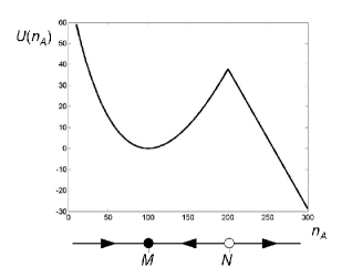
Figure 1: The potential energy landscape corresponding to the model described in Eq. (1). There exist two fixed points: a stable one at $n_{A}=M$ and an unstable one at $n_{A}=N$. If $n_{A}$ gets beyond $N$, it will diverge to infinity. The phase portrait of the model is depicted under the plot.

This deterministic picture is of course incomplete due to the neglect of the intrinsic fluctuations from the reaction propensities. Such fluctuations are approximately captured by the following CLE Gillespie (2000):

$$\dot{n}_{A}=\big{[}\lambda(n_{A})-\Gamma n_{A}\big{]}n_{A}+\sqrt{\lambda(n_{A})n_{A}}w+\sqrt{\Gamma n_{A}^{2}}w^{\prime}\ ,$$ (4)

where $w,w^{\prime}$ are Gaussian noises with zero means and unit standard deviations. Since $w$ and $w^{\prime}$ are uncorrelated, we have

$$\dot{n}_{A}=\gamma f+\sqrt{2\gamma}w$$ (5)

where we have introduced the following functions:

$$\gamma = \frac{\big{[}\lambda(n_{A})+\Gamma n_{A}\big{]}n_{A}}{2}$$ (6)

$$f = \frac{2[\lambda(n_{A})-\Gamma n_{A}]}{\lambda(n_{A})+\Gamma n_{A}}\ .$$ (7)

Note that the form of Eq. (5) corresponds to a Langevin equation describing a particle in a potential well under thermal perturbations in the non-inertia regime. Specifically, $n_{A}$ can be treated as the coordinate of the particle, $f$ as the force exerted on the particle due to an underlying potential, and $\gamma$ as the position-dependent damping coefficient of the system.

In the region $n_{A}<M$, the force is

$$f(n_{A})=\frac{2(M-n_{A})}{M+n_{A}}\ .$$ (8)

The corresponding potential energy can thus be determined as

$$U(n_{A}) = -\int_{M}^{n_{A}}{\rm d}xf(x)$$ (9)

$$= 2(n_{A}-M)-4M\ln\frac{n_{A}+M}{2M}\ .$$ (10)

Similarly, in the region $n_{A}\geq M$, we have $f(n_{A})=\frac{2}{3}$ and $U(n_{A})=-2n_{A}/3+{\rm constant}$. The shape of the potential energy is depicted in Fig. 1.

We are primarily concerned with rare escape events and we thus assume that $N-M\gg 1$. In this scenario, if the initial state of the system is such that $n_{A}(t=0)=M$, then the waiting time, $\tau$, for the system to move out of the potential well, i.e., the waiting time for $n_{A}$ to attain the value $N$ is (c.f. Sect. 7.2 in Hänggi et al. (1990)):

$$\tau = \frac{2\pi}{U^{\prime\prime}(M)}\exp\left[2(N-M)-4M\ln\frac{N+M}{2M}\right]$$ (11)

$$= 2\pi M\exp\left[2(N-M)-4M\ln\frac{N+M}{2M}\right]\ .$$ (12)

Note that $n_{A}$ will, with probability one, either go to zero or diverge Hänggi et al. (1990), and so the knowledge of the escape rate is particularly important.

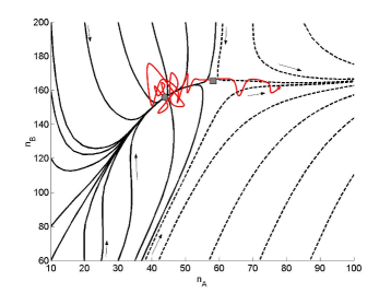
Figure 2: (Color online) The flow lines of the cell proliferation model described in Eqs (13) and (14). The two fixed points of the models are depicted by the gray circle and square (c.f. Eqs (22) and (23)). The red (gray) wriggly line depicts schematically a possible escape trajectory. The numerical values for the model parameters are $\alpha=2$, $\beta=10$, $r=0.08$, $n_{0}=200$, $\Gamma=0.045$, $\rho_{0}=0.22$ and $\rho_{1}=0.26$ Warren (2009).

III Skin cell proliferation

We now move onto discussing a model for skin cell proliferation. The model we study is based on the single progenitor cell model introduced in Clayton et al. (2007); Klein et al. (2007). This model was then generalized in Warren (2009) to account for the homeostasis of the system. Furthermore, the author in Warren (2009) suggests that the escape of the system from the homeostatic basin due to rare stochastic fluctuations plays a role in uncontrolled cell proliferation. This is of important relevance to the study of skin cancer. Specifically, there are two basal layer cell types in this model: progenitor cells $A$ and postmitotic cells $B$. These two types of cells proliferate according to following scheme:

$$A\stackrel{{\scriptstyle\lambda_{1}}}{{\longrightarrow}}A+A A\stackrel{{\scriptstyle\lambda_{2}}}{{\longrightarrow}}A+B$$ , (13)

$$A\stackrel{{\scriptstyle\lambda_{3}}}{{\longrightarrow}}B+B B\stackrel{{\scriptstyle\Gamma}}{{\longrightarrow}}\emptyset\ .$$ , (14)

The first three processes represent the different progenitor cell division pathways, and the fourth represents postmitotic cells leaving the basal layer. In the model above, $\Gamma$ is a constant and $\lambda_{i}$ are defined as follow:

$$\lambda_{1} = \lambda(n)r(1-q(\rho))$$ (15)

$$\lambda_{2} = \lambda(n)(1-2r)$$ (16)

$$\lambda_{3} = \lambda(n)r(1+q(\rho))$$ (17)

where

$$n=n_{A}+n_{B} \rho=\frac{n_{A}}{n}$$ , (18)

$$\lambda(n)=\lambda_{0}\left(\frac{n_{0}}{n}\right)^{2} \lambda_{0}=\frac{\Gamma(1-\rho_{0})}{\rho_{0}}$$ , (19)

and

$$q(\rho)=\tanh\left[\frac{10\rho_{0}(1-\rho_{0})(\rho-\rho_{0})(\rho_{1}-\rho)}{\rho(1-\rho)(\rho_{1}-\rho_{0})}\right]\ .$$ (20)

Note that the constants $n_{0}$, $\rho_{0}$ and $\rho_{1}$ represent the initial number of cells, the fraction of progenitor cells at the stable fixed point (marked by the gray circle in Fig. 2), and the fraction of progenitor cells at the unstable fixed point (marked by the gray square in Fig. 2), respectively. An experimentally motivated set of parameters for this model is shown in the caption of Fig. 2. We refer the readers to Clayton et al. (2007); Klein et al. (2007); Warren (2009) for more detailed physiological interpretations of the different processes. Here, we will only note that a divergence of the total cell density, $n_{A}+n_{B}$, signifies the onset of uncontrolled cell proliferation. In Warren (2009), the author employs the standard Gillespie kinetic Monte Carlo algorithm Gillespie (1977) to perform stochastic simulations of the model, and finds that the escape rate has an exponential component of the form $\exp(-4.6\times n_{0}\triangle\rho^{2})$ where $\triangle\rho\equiv\rho_{1}-\rho_{0}$ denotes the difference in the fractions of progenitor cells at the saddle point and at the fixed point. We will now demonstrate how the Kramers escape theory accounts for the exponent observed.

We shall first look at the deterministic case, where the chemical reaction scheme in Eqs (13) and (14) lead to the following set of ordinary differential equations:

$$\dot{n}_{A}=-2\lambda rqn_{A}\ \ \ ,\ \ \ \dot{n}_{B}=\lambda(1+2rq)n_{A}-\Gamma n_{B}\ .$$ (21)

Setting the L.H.S. in the equations above to zero, we find two nontrivial fixed points:

$$\mathbf{X} = \big{(}n_{0}\rho_{0}\ ,\ (1-\rho_{0})n_{0}\big{)}$$ (22)

$$\mathbf{Y} = \left(n_{0}\sqrt{\frac{\lambda_{0}\rho_{1}^{3}}{\Gamma(1-\rho_{1})}}\ ,\ n_{0}\sqrt{\frac{\lambda_{0}\rho_{1}(1-\rho_{1})}{\Gamma}}\right)\ .$$ (23)

These fixed points are denoted by a gray circle and a gray square respectively in Fig. 2 along with flow lines.

The corresponding CLE for this system is Gillespie (2000):

$$\dot{n}_{A} = (\lambda_{1}-\lambda_{3})n_{A}+\sqrt{\lambda_{1}n_{A}}w_{1}-\sqrt{\lambda_{3}n_{A}}w_{3}$$ (24)

$$\dot{n}_{B} = (\lambda_{2}+2\lambda_{3})n_{A}-\Gamma n_{B}$$ (26)

$$+\sqrt{\lambda_{2}n_{A}}w_{2}+2\sqrt{\lambda_{3}n_{A}}w_{3}-\sqrt{\Gamma n_{B}}w_{4}\ ,$$

where the $w_{i}$ are again Gaussian noises with zero means and unit standard deviations. As among the four independent Gaussian noise terms, only $w_{3}$ are common in both equations, we can thus simplify the above equation to the followings:

$$\dot{n}_{A} = (\lambda_{1}-\lambda_{3})n_{A}+\sqrt{(\lambda_{1}+\lambda_{3})n_{A}}w_{1}$$ (27)

$$\dot{n}_{B} = (\lambda_{2}+2\lambda_{3})n_{A}-\Gamma n_{B}$$

$$+\sqrt{(\lambda_{2}+4\lambda_{3})n_{A}+\Gamma n_{B}}\left[\sigma w_{1}+\sqrt{1-\sigma^{2}}w_{2}\right]$$

where

$$\sigma=\frac{2\lambda_{3}n_{A}}{\sqrt{n_{A}(\lambda_{1}+\lambda_{3})[(\lambda_{2}+4\lambda_{3})n_{A}+\Gamma n_{B}]}}$$ (29)

corresponds to the correlation between the two fluctuation processes.

Note that in dimensions higher than one, one cannot in general represent the force fields as the gradients of a potential, i.e., the force is not conservative. Although a potential energy cannot be constructed here, it is still possible to obtain a scalar function that serves to determine the exponent in the Arrhenius term associated to the escape process Matkowsky and Schuss (1977). This can be achieved by solving a second-order boundary value problem, and usually can only be done numerically. Here, we will avoid this numerical challenge and aim to proceed analytically by making a series of approximations to the above CLE.

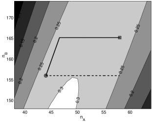
Figure 3: The magnitude of the correlation $\sigma$ as a function of $n_{A}$ and $n_{B}$ around the two fixed points indicated again by the square and the circle. The broken line denotes the escape path corresponding to the analytical calculation in Eq. (36), and the solid line denotes the escape path obtained numerically (c.f. the discussion before Eq. (39)), which corresponds to the result in Eq. (40).

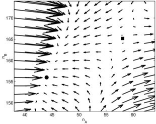
Figure 4: The force vector fields, $(f_{A},f_{B})$, according to Eqs (32). The magnitudes of the vectors are scaled up uniformly for visual clarity.

As aforementioned, the Gaussian noises associated to the two coordinates are correlated. In Fig. 3, we show the magnitude of $\sigma$ around the two fixed points, which is bounded above by 0.31. The first approximation is that we will set $\sigma$ to zero, i.e., we assume that the perturbations acting on $n_{A}$ and $n_{B}$ are uncorrelated. With this simplification, Eqs (24) and (26) can be written as:

$$\dot{n}_{A}=\gamma_{A}f_{A}+\sqrt{2\gamma_{A}}w_{A}\ \ \ ,\ \ \ \dot{n}_{B}=\gamma_{B}f_{B}+\sqrt{2\gamma_{B}}w_{B}\ ,$$ (30)

where

$$\gamma_{A}=r\lambda n_{A} \gamma_{B}=\frac{\lambda(1+2r+4rq)n_{A}+\Gamma n_{B}}{2}$$ , (31)

$$f_{A}=-2q f_{B}=\frac{2\lambda(1+2rq)n_{A}-2\Gamma n_{B}}{\lambda(1+2r+4rq)n_{A}+\Gamma n_{B}}\ .$$ , (32)

Fig. 4 show the force vectors $(f_{A},f_{B})$ around the two fixed points, which suggests that $|f_{B}|\ll|f_{A}|$ in the region connecting $\mathbf{X}$ and $\mathbf{Y}$. In other words, it is much easier for the particle to diffuse vertically than to diffuse horizontally. We will therefore ignore the second dimension and consider purely the first coordinate. This constitutes our second approximation and effectively collapses the problem into a one-dimensional problem. As a result, we can calculate the corresponding potential by simply integrating over $f_{A}$:

$$U=\int 2q\left(\frac{x}{x+\hat{n}_{B}}\right){\rm d}x\ .$$ (33)

where we will take $\hat{n}_{B}=X_{B}$ (c.f. Eqs (20) and (22)). If the initial cell densities are in the metastable region around $\mathbf{X}$, the rate, $R$, at which uncontrolled cell proliferation occurs will be of the form $R\propto\exp(-\triangle U)$ Matkowsky and Schuss (1977), where

$$\triangle U=\int_{X_{A}}^{Y_{A}}2q\left(\frac{x}{x+\hat{n}_{B}}\right){\rm d}x\ .$$ (34)

Note that our consideration effectively amounts to calculating the first passage time of a particle constrained to diffuse along the horizontal path depicted by the broken line in Fig. 3.

Since throughout the range of the integration, the argument in $q$ is bounded above by 0.12, $q$ is well approximated by $\tilde{q}$ where (c.f. Eq. (20))

$$\tilde{q}(\rho)=\frac{10\rho_{0}(1-\rho_{0})(\rho-\rho_{0})(\rho_{1}-\rho)}{\rho(1-\rho)(\rho_{1}-\rho_{0})}\ .$$ (35)

This simplification allows us to perform the integration in Eq. (34) analytically, and we find that for small $\triangle\rho$,

$$\triangle U = \frac{5\rho_{0}(3-2\rho_{0})^{2}}{3(1-\rho_{0})}n_{0}\triangle\rho^{2}+{\cal O}(\triangle\rho^{3})$$ (36)

$$\simeq 3.1\times n_{0}\triangle\rho^{2}\ ,$$ (37)

where the second approximated equality comes from substituting in the numerical values of the parameters shown in the caption of Fig. 2. Recall that the exponent is found numerically to be $(4.6\times n_{0}\triangle\rho^{2})$ Warren (2009). We have therefore recovered the scaling of the exponent with respect to $\triangle\rho$. On the other hand, the prefactor we obtained is about two thirds of that observed from simulations.

We will now try to incorporate the second dimension and the correlation in the fluctuations into the picture. Our strategy is to find a path that better represents the escape route. In the weak noise limit, such an optimal escape path encapsulates the information on the asymptotic behavior of the escape process, and in principle, can be obtained by solving a set Hamiltonian equations with the appropriate end points. Caroli et al. (1980); Maier and Stein (1992, 1993); Altland and Simons (2010). We find the application of the numerical procedure to the problem concerned challenging as the corresponding set of Hamiltonian equations are higher sensitive to the initial conditions chosen. Hence, we will instead make a crude estimate on the escape path that connects the metastable state to the saddle point . Specifically, as we have argued that the particle diffuses more easily along the vertical direction, we reason that as the particle goes upward in the $nA$ direction, it should stay at the bottom of the valley with respect to the force fields along the $n_{A}$. We therefore start at the metastable point, $\mathbf{X}$, and find the $n_{A}$ that minimizes $|f_{A}|$ as we move up in the $n_{B}$ dimension. We find that such a path corresponds to a slanted as depicted by the solid line in Fig. 3. When the path reaches $Y_{B}$ in the $n_{B}$ coordinate, we simply connects it horizontally with the saddle point $\mathbf{Y}$ (c.f. Fig. 3). We denote this escape path by $\mathbf{z}(s)$, where $0\leq s\leq L$ corresponds to the parametrization of the curve such that $\mathbf{z}(0)={\bf X}$, $\mathbf{z}(L)={\bf Y}$ and $|\mathbf{z}^{\prime}(s)|=1$ for all $s$. Now, we collapse again the problem into one dimension by considering only fluctuation processes along this path. The time evolution of the particle along the path can be expressed as:

$$\dot{s} = u\gamma_{A}f_{A}+v\gamma_{B}f_{B}$$

$$+\left[2(u^{2}\gamma_{A}+v^{2}\gamma_{B}+2\sigma uv\sqrt{\gamma_{A}\gamma_{B}})\right]^{1/2}w\ ,$$

where the $\gamma_{A/B}$ and $f_{A/B}$ are as expressed in Eqs (31) and (32), $\sigma$ is defined in Eq. (29), and $(u,v)$ denotes the unit tangent of the curve $\mathbf{z}$ at the point $(n_{A},n_{B})$. As a result, the exponent in the rate describing the escape process from $s=0$ to $s=L$ is:

$$\triangle U=-\int_{0}^{L}\frac{u\gamma_{A}f_{A}+v\gamma_{B}f_{B}}{u^{2}\gamma_{A}+v^{2}\gamma_{B}+2\sigma uv\sqrt{\gamma_{A}\gamma_{B}}}\ {\rm d}s\ .$$ (39)

The numerical value is found to be

$$\triangle U=2.05=6.4\times n_{0}\triangle\rho^{2}\ ,$$ (40)

which is greater than the simulation results by about 39%. The discrepancy here is likely an outcome of our crude way of estimating the escape path. To improve upon this result, more sophisticated numerical approaches would be required, which is beyond the scope of this work.

IV Conclusion

In summary, we have discussed how the Kramers escape theory can be used to predict rare events in chemical reactions due to stochastic fluctuations. As an application, we have considered a model on cell proliferation and explained analytically the observed rate for the onset of uncontrolled cell growth.

References

- van Kampen (2007) N. G. van Kampen, Stochastic Processes in Physics and Chemistry (North Holland, 2007), 3rd ed.
- Gardiner (2009) C. Gardiner, Stochastic Methods: A Handbook for the Natural and Social Sciences (Springer, 2009), 4th ed.
- Kurtz (1978) T. Kurtz, Stochastic Processes and their Applications 6, 223 (1978).
- Gillespie (2000) D. T. Gillespie, The Journal of Chemical Physics 113, 297 (2000).
- Grabert et al. (1983) H. Grabert, P. Hänggi, and I. Oppenheim, Physica A: Statistical and Theoretical Physics 117, 300 (1983).
- Hänggi et al. (1984) P. Hänggi, H. Grabert, P. Talkner, and H. Thomas, Physical Review A 29, 371 (1984).
- Caroli et al. (1980) B. Caroli, C. Caroli, B. Roulet, and J. F. Gouyet, Journal of Statistical Physics 22, 515 (1980).
- Hänggi et al. (1990) P. Hänggi, P. Talkner, and M. Borkovec, Reviews of Modern Physics 62, 251 (1990).
- Reichenbach et al. (2006) T. Reichenbach, M. Mobilia, and E. Frey, Physical Review E 74, 051907 (2006).
- Kessler and Shnerb (2007) D. Kessler and N. Shnerb, Journal of Statistical Physics 127, 861 (2007).
- Kamenev and Meerson (2008) A. Kamenev and B. Meerson, Physical Review E 77, 061107 (2008).
- Dykman et al. (2008) M. I. Dykman, I. B. Schwartz, and A. S. Landsman, Physical Review Letters 101, 078101 (2008).
- Schwartz et al. (2009) I. B. Schwartz, L. Billings, M. Dykman, and A. Landsman, Journal of Statistical Mechanics: Theory and Experiment 2009, P01005 (2009).
- Bialek (2000) W. Bialek, Stability and noise in biochemical switches (MIT Press, 2000), pp. 103–109, eprint cond-mat/0005235.
- Warren (2009) P. B. Warren, Physical Review E (Statistical, Nonlinear, and Soft Matter Physics) 80, 030903 (2009).
- Clayton et al. (2007) E. Clayton, D. P. Doupe, A. M. Klein, D. J. Winton, B. D. Simons, and P. H. Jones, Nature 446, 185 (2007).
- Klein et al. (2007) A. M. Klein, D. P. Doupé, P. H. Jones, and B. D. Simons, Physical Review E (Statistical, Nonlinear, and Soft Matter Physics) 76, 021910 (2007).
- Gillespie (1977) D. T. Gillespie, The Journal of Physical Chemistry 81, 2340 (1977).
- Matkowsky and Schuss (1977) B. J. Matkowsky and Z. Schuss, SIAM Journal on Applied Mathematics 33, 365 (1977).
- Maier and Stein (1992) R. S. Maier and D. L. Stein, Physical Review Letters 69, 3691 (1992).
- Maier and Stein (1993) R. S. Maier and D. L. Stein, Physical Review E 48, 931 (1993).
- Altland and Simons (2010) A. Altland and B. Simons, Condensed Matter Field Theory (Cambridge University Press, 2010), 2nd ed.
- Maier and Stein (1997) R. S. Maier and D. L. Stein, SIAM Journal on Applied Mathematics 57, 752 (1997).