LACBoost and FisherBoost: Optimally Building Cascade Classifiers

Abstract

Object detection is one of the key tasks in computer vision. The cascade framework of Viola and Jones has become the de facto standard. A classifier in each node of the cascade is required to achieve extremely high detection rates, instead of low overall classification error. Although there are a few reported methods addressing this requirement in the context of object detection, there is no a principled feature selection method that explicitly takes into account this asymmetric node learning objective. We provide such a boosting algorithm in this work. It is inspired by the linear asymmetric classifier (LAC) of [1] in that our boosting algorithm optimizes a similar cost function. The new totally-corrective boosting algorithm is implemented by the column generation technique in convex optimization. Experimental results on face detection suggest that our proposed boosting algorithms can improve the state-of-the-art methods in detection performance.

1 Introduction

Real-time detection of various categories of objects in images is one of the key tasks in computer vision. This topic has been extensively studied in the past a few years due to its important applications in surveillance, intelligent video analysis etc. Viola and Jones proffered the first real-time face detector [2, 3]. To date, it is still considered one of the state-of-the-art, and their framework is the basis of many incremental work afterwards. Object detection is a highly asymmetric classification problem with the exhaustive scanning-window search being used to locate the target in an image. Only a few are true target objects among the millions of scanned patches. Cascade classifiers have been proposed for efficient detection, which takes the asymmetric structure into consideration. Under the assumption of each node of the cascade classifier makes independent classification errors, the detection rate and false positive rate of the entire cascade are: $F_{\rm dr}=\prod_{t=1}^{N}d_{t}$ and $F_{\rm fp}=\prod_{t=1}^{N}f_{t}$, respectively. As pointed out in [2, 1], these two equations suggest a node learning objective: Each node should have an extremely high detection rate $d_{t}$ (e.g., $99.7\%$) and a moderate false positive rate $f_{t}$ (e.g., $50\%$). With the above values of $d_{t}$ and $f_{t}$, assume that the cascade has $N=20$ nodes, then $F_{\rm dr}\approx 94\%$ and $F_{\rm fp}\approx 10^{-6}$, which is usually the design goal.

A drawback of standard boosting like AdaBoost is that it does not take advantage of the cascade classifier. AdaBoost only minimizes the overall classification error and does not minimize the number of false negatives. In this sense, the features selected are not optimal for the purpose of rejecting negative examples. At the feature selection and classifier training level, Viola and Jones leveraged the asymmetry property, to some extend, by replacing AdaBoost with AsymBoost [3]. AsymBoost incurs more loss for misclassifying a positive example by simply modifying AdaBoost’s exponential loss. Better detection rates were observed over the standard AdaBoost. Nevertheless, AsymBoost addresses the node learning goal indirectly and still may not be the optimal solution. Wu et al. explicitly studied the node learning goal and they proposed to use linear asymmetric classifier (LAC) and Fisher linear discriminant analysis (LDA) to adjust the linear coefficients of the selected weak classifiers [1, 4]. Their experiments indicated that with this post-processing technique, the node learning objective can be better met, which is translated into improved detection rates. In Viola and Jones’ framework, boosting is used to select features and at the same time to train a strong classifier. Wu et al.’s work separates these two tasks: they still use AdaBoost or AsymBoost to select features; and at the second step, they build a strong classifier using LAC or LDA. Since there are two steps here, in Wu et al.’s work [1, 4], the node learning objective is only considered at the second step. At the first step—feature selection—the node learning objective is not explicitly considered. We conjecture that further improvement may be gained if the node learning objective is explicitly taken into account at both steps. We design new boosting algorithms to implement this idea and verify this conjecture. Our major contributions are as follows.

1. We develop new boosting-like algorithms via directly minimizing the objective function of linear asymmetric classifier, which is termed as LACBoost (and FisherBoost from Fisher LDA). Both of them can be used to select features that is optimal for achieving the node learning goal in training a cascade classifier. To our knowledge, this is the first attempt to design such a feature selection method.

2. LACBoost and FisherBoost share similarities with LPBoost [5] in the sense that both use column generation—a technique originally proposed for large-scale linear programming (LP). Typically, the Lagrange dual problem is solved at each iteration in column generation. We instead solve the primal quadratic programming (QP) problem, which has a special structure and entropic gradient (EG) can be used to solve the problem very efficiently. Compared with general interior-point based QP solvers, EG is much faster. Considering one needs to solve QP problems a few thousand times for training a complete cascade detector, the efficiency improvement is enormous. Compared with training an AdaBoost based cascade detector, the time needed for LACBoost (or FisherBoost) is comparable. This is because for both cases, the majority of the time is spent on weak classifier training and bootstrapping.

3. We apply LACBoost and FisherBoost to face detection and better performances are observed over the state-of-the-art methods [1, 4]. The results confirm our conjecture and show the effectiveness of LACBoost and FisherBoost. LACBoost can be immediately applied to other asymmetric classification problems.

4. We also analyze the condition that makes the validity of LAC, and show that the multi-exit cascade might be more suitable for applying LAC learning of [1, 4] (and our LACBoost) rather than Viola-Jones standard cascade.

Besides these, the LACBoost/FisherBoost algorithm differs from traditional boosting algorithms in that LACBoost/FisherBoost does not minimize a loss function. This opens new possibilities for designing new boosting algorithms for special purposes. We have also extended column generation for optimizing nonlinear optimization problems. Next we review some related work that is closest to ours.

Related work There is a large body of previous work in object detection [6, 7]; of particular relevance to our work is boosting object detection originated from Viola and Jones’ framework. There are three important components that make Viola and Jones’ framework tremendously successful: (1) The cascade classifier that efficiently filters out most negative patches in early nodes; and also contributes to enable the final classifier to have a very high detection rate; (2) AdaBoost that selects informative features and at the same time trains a strong classifier; (3) The use of integral images, which makes the computation of Haar features extremely fast. Most of the work later improves one or more of these three components. In terms of the cascade classifier, a few different approaches such as soft cascade [8], dynamic cascade [9], and multi-exit cascade [10]. We have used the multi-exit cascade in this work. The multi-exit cascade tries to improve the classification performance by using all the selected weak classifiers for each node. So for the $n$-th strong classifier (node), it uses all the weak classifiers in this node as well as those in the previous $n-1$ nodes. We show that the LAC post-processing can enhance the multi-exit cascade. More importantly, we show that the multi-exit cascade better meets LAC’s requirement of data being Gaussian distributions.

The second research topic is the learning algorithm for constructing a classifier. Wu et al. use fast forward feature selection to accelerate the training procedure [7]. They have also proposed LAC to learn a better strong classifier [1]. Pham and Cham recently proposed online asymmetric boosting with considerable improvement in training time [6]. By exploiting the feature statistics, they have also designed a fast method to train weak classifiers [11]. Li et al. advocated FloatBoost to discard some redundant weak classifiers during AdaBoost’s greedy selection procedure [12]. Liu and Shum proposed KLBoost to select features and train a strong classifier [13]. Other variants of boosting have been applied to detection.

Notation The following notation is used. A matrix is denoted by a bold upper-case letter ($\mathbf{X}$); a column vector is denoted by a bold lower-case letter ($\mathbf{x}$). The $i$th row of $\mathbf{X}$ is denoted by $\mathbf{X}_{i:}$ and the $i$-th column $\mathbf{X}_{:i}$. The identity matrix is $\bf I$ and its size should be clear from the context. $\bf 1$ and $\bf 0$ are column vectors of $1$’s and $0$’s, respectively. We use $\succcurlyeq,\preccurlyeq$ to denote component-wise inequalities.

Let $\{(\mathbf{x}_{i},y_{i})\}_{i=1,\cdots,m}$ be the set of training data, where $\mathbf{x}_{i}\in\mathcal{X}$ and $y_{i}\in\{-1,+1\}$, $\forall i$. The training set consists of $m_{1}$ positive training points and $m_{2}$ negative ones; $m_{1}+m_{2}=m$. Let $h(\cdot)\in\mathcal{H}$ be a weak classifier that projects an input vector $\mathbf{x}$ into $\{-1,+1\}$. Here we only consider discrete classifier outputs. We assume that the set $\mathcal{H}$ is finite and we have $n$ possible weak classifiers. Let the matrix $\mathbf{H}\in\mathbb{R}^{m\times n}$ where the $(i,j)$ entry of $\mathbf{H}$ is $\mathbf{H}_{ij}=h_{j}(\mathbf{x}_{i})$. $\mathbf{H}_{ij}$ is the label predicted by weak classifier $h_{j}(\cdot)$ on the training datum $\mathbf{x}_{i}$. We define a matrix $\mathbf{A}\in\mathbb{R}^{m\times n}$ such that its $(i,j)$ entry is $\mathbf{A}_{ij}=y_{i}h_{j}(\mathbf{x}_{i})$.

2 Linear Asymmetric Classification

Before we propose our LACBoost and FisherBoost, we briefly overview the concept of LAC. Wu et al. [4] have proposed linear asymmetric classification (LAC) as a post-processing step for training nodes in the cascade framework. LAC is guaranteed to get an optimal solution under the assumption of Gaussian data distributions.

Suppose that we have a linear classifier $f(\mathbf{x})={\bf sign}(\mathbf{w}^{\!\top}\mathbf{x}-b)$, if we want to find a pair of $\{\mathbf{w},b\}$ with a very high accuracy on the positive data $\mathbf{x}_{1}$ and a moderate accuracy on the negative $\mathbf{x}_{2}$, which is expressed as the following problem:

$$\begin{split}\max_{\mathbf{w}\neq{\bf 0},b}\,\Pr_{\mathbf{x}_{1}\sim(\mu_{1},{\bf\Sigma}_{1})}\{\mathbf{w}^{\!\top}\mathbf{x}_{1}\geq b\},\,\,{\rm s.t.}\,\Pr_{\mathbf{x}_{2}\sim(\mu_{2},{\bf\Sigma}_{2})}\{\mathbf{w}^{\!\top}\mathbf{x}_{2}\leq b\}=\lambda,\end{split}$$ (1)

where $\mathbf{x}\sim(\mu,{\bf\Sigma})$ denotes a symmetric distribution with mean $\mu$ and covariance ${\bf\Sigma}$. If we prescribe $\lambda$ to $0.5$ and assume that for any $\mathbf{w}$, $\mathbf{w}^{\!\top}\mathbf{x}_{1}$ is Gaussian and $\mathbf{w}^{\!\top}\mathbf{x}_{2}$ is symmetric, then (1) can be approximated by

$$\max_{\mathbf{w}\neq\bf 0}\;\;\frac{\mathbf{w}^{\!\top}(\mu_{1}-\mu_{2})}{\sqrt{\mathbf{w}^{\!\top}{\bf\Sigma}_{1}\mathbf{w}}}.$$ (2)

(2) is similar to LDA’s optimization problem

$$\max_{\mathbf{w}\neq\bf 0}\;\;\frac{\mathbf{w}^{\!\top}(\mu_{1}-\mu_{2})}{\sqrt{\mathbf{w}^{\!\top}({\bf\Sigma}_{1}+{\bf\Sigma}_{2})\mathbf{w}}}.$$ (3)

(2) can be solved by eigen-decomposition and a close-formed solution can be derived:

$$\mathbf{w}^{\star}={\bf\Sigma}_{1}^{-1}(\mu_{1}-\mu_{2}),\quad b^{\star}={\mathbf{w}^{\star}}^{{\!\top}}\mu_{2}.$$ (4)

On the other hand, each node in cascaded boosting classifiers has the following form:

$$f(\mathbf{x})={\bf sign}(\mathbf{w}^{\!\top}\mathbf{H}(\mathbf{x})-b),$$ (5)

We override the symbol $\mathbf{H}(\mathbf{x})$ here, which denotes the output vector of all weak classifiers over the datum $\mathbf{x}$. We can cast each node as a linear classifier over the feature space constructed by the binary outputs of all weak classifiers. For each node in cascade classifier, we wish to maximize the detection rate as high as possible, and meanwhile keep the false positive rate to an moderate level (e.g., $50.0\%$). That is to say, the problem (1) expresses the node learning goal. Therefore, we can use boosting algorithms (e.g., AdaBoost) as feature selection methods, and then use LAC to learn a linear classifier over those binary features chosen by boosting. The advantage is that LAC considers the asymmetric node learning explicitly.

However, there is a precondition of LAC’s validity. That is, for any $\mathbf{w}$, $\mathbf{w}^{\!\top}\mathbf{x}_{1}$ is a Gaussian and $\mathbf{w}^{\!\top}\mathbf{x}_{2}$ is symmetric. In the case of boosting classifiers, $\mathbf{w}^{\!\top}\mathbf{x}_{1}$ and $\mathbf{w}^{\!\top}\mathbf{x}_{2}$ can be expressed as the margin of positive data and negative data. Empirically Wu et al. [4] verified that $\mathbf{w}^{\!\top}\mathbf{x}$ is Gaussian approximately for a cascade face detector. We discuss this issue in the experiment part in more detail.

3 Constructing Boosting Algorithms from LDA and LAC

In kernel methods, the original data are nonlinearly mapped to a feature space and usually the mapping function ${\phi}(\cdot)$ is not explicitly available. It works through the inner product of ${\phi}(\mathbf{x}_{i})^{\!\top}{\phi}(\mathbf{x}_{j})$. In boosting [14], the mapping function can be seen as explicitly known through: ${\phi}(\mathbf{x}):\mathbf{x}\mapsto[h_{1}(\mathbf{x}),\dots,h_{n}(\mathbf{x})].$ Let us consider the Fisher LDA case first because the solution to LDA will generalize to LAC straightforwardly, by looking at the similarity between (2) and (3).

Fisher LDA maximizes the between-class variance and minimizes the within-class variance. In the binary-class case, we can equivalently rewrite (3) into

$$\max_{\mathbf{w}}\;\;\frac{(\mu_{1}-\mu_{2})^{2}}{\sigma_{1}+\sigma_{2}}=\frac{\mathbf{w}^{\!\top}\mathbf{C}_{b}\mathbf{w}}{\mathbf{w}^{\!\top}\mathbf{C}_{w}\mathbf{w}},$$ (6)

where $\mathbf{C}_{b}$ and $\mathbf{C}_{w}$ are the between-class and within-class scatter matrices; $\mu_{1}$ and $\mu_{2}$ are the projected centers of the two classes. The above problem can be equivalently reformulated as

$$\min_{\mathbf{w}}\;\;\mathbf{w}^{\!\top}\mathbf{C}_{w}\mathbf{w}-\theta(\mu_{1}-\mu_{2})$$ (7)

for some certain constant $\theta$ and under the assumption that $\mu_{1}-\mu_{2}\geq 0$. Now in the feature space, our data are ${\phi}(\mathbf{x}_{i})$, $i=1\dots m$. We have

$$\mu_{1} =\frac{1}{m_{1}}\mathbf{w}^{\!\top}\sum_{y_{i}=1}{\phi}(\mathbf{x}_{i})=\frac{1}{m_{1}}\sum_{y_{i}=1}\mathbf{A}_{i:}\mathbf{w}=\frac{1}{m_{1}}\sum_{y_{i}=1}(\mathbf{A}\mathbf{w})_{i}=\boldsymbol{e}_{1}^{\!\top}\mathbf{A}\mathbf{w},$$ (8)

where $\mathbf{A}_{i:}$ is the $i$-th row of $\mathbf{A}$.

$$\mu_{2} =\frac{1}{m_{2}}\mathbf{w}^{\!\top}\sum_{y_{i}=-1}{\phi}(\mathbf{x}_{i})=\frac{1}{m_{2}}\sum_{y_{i}=-1}\mathbf{H}_{i:}\mathbf{w}=-\boldsymbol{e}_{2}^{\!\top}\mathbf{A}\mathbf{w},$$ (9)

Here the $i$-th entry of $\boldsymbol{e}_{1}$ is defined as $\boldsymbol{e}_{1i}=1/m_{1}$ if $y_{i}=+1$, otherwise $\boldsymbol{e}_{1i}=0$. Similarly $\boldsymbol{e}_{2i}=1/m_{2}$ if $y_{i}=-1$, otherwise $\boldsymbol{e}_{2i}=0$. We also define $\boldsymbol{e}=\boldsymbol{e}_{1}+\boldsymbol{e}_{2}$. For ease of exposition, we order the training data according to their labels. So the vector $\boldsymbol{e}\in\mathbb{R}^{m}$:

$$\boldsymbol{e}=[1/m_{1},\cdots,1/m_{2},\cdots]^{\!\top},$$ (10)

and the first $m_{1}$ components of $\boldsymbol{\rho}$ correspond to the positive training data and the remaining ones correspond to the $m_{2}$ negative data. So we have $\mu_{1}-\mu_{2}=\boldsymbol{e}^{\!\top}\boldsymbol{\rho}$, $\mathbf{C}_{w}={m_{1}}/{m}\cdot{\bf\Sigma}_{1}+{m_{2}}/{m}\cdot{\bf\Sigma}_{2}$ with ${\bf\Sigma}_{1,2}$ the covariance matrices. By noticing that

$$\mathbf{w}^{\!\top}{\bf\Sigma}_{1,2}\mathbf{w}=\frac{1}{m_{1,2}(m_{1,2}-1)}\sum_{i>k,y_{i}=y_{k}=\pm 1}(\rho_{i}-\rho_{k})^{2},$$

we can easily rewrite the original problem into:

$$\min_{\mathbf{w},\boldsymbol{\rho}}\tfrac{1}{2}\boldsymbol{\rho}^{\!\top}\mathbf{Q}\boldsymbol{\rho}-\theta\boldsymbol{e}^{\!\top}\boldsymbol{\rho},\quad{\rm s.t.}~{} \mathbf{w}\succcurlyeq{\bf 0},{\bf 1}^{\!\top}\mathbf{w}=1,{\rho}_{i}=(\mathbf{A}\mathbf{w})_{i},i=1,\cdots,m.$$ (11)

Here $\mathbf{Q}=\begin{bmatrix}\mathbf{Q}_{1}&{\bf 0}\\ {\bf 0}&\mathbf{Q}_{2}\end{bmatrix}$ is a block matrix with

$$\mathbf{Q}_{1}=\begin{bmatrix}\tfrac{1}{m}&-\tfrac{1}{m(m_{1}-1)}&\ldots&-\tfrac{1}{m(m_{1}-1)}\\ -\tfrac{1}{m(m_{1}-1)}&\tfrac{1}{m}&\ldots&-\tfrac{1}{m(m_{1}-1)}\\ \vdots&\vdots&\ddots&\vdots\\ -\tfrac{1}{m(m_{1}-1)}&-\tfrac{1}{m(m_{1}-1)}&\ldots&\tfrac{1}{m}\end{bmatrix},$$

and $\mathbf{Q}_{2}$ is similarly defined by replacing $m_{1}$ with $m_{2}$ in $\mathbf{Q}_{1}$. Also note that we have introduced a constant $\frac{1}{2}$ before the quadratic term for convenience. The normalization constraint ${\bf 1}^{\!\top}\mathbf{w}=1$ removes the scale ambiguity of $\mathbf{w}$. Otherwise the problem is ill-posed.

In the case of LAC, the covariance matrix of the negative data is not involved, which corresponds to the matrix $\mathbf{Q}_{2}$ is zero. So we can simply set $\mathbf{Q}=\begin{bmatrix}\mathbf{Q}_{1}&{\bf 0}\\ {\bf 0}&\bf 0\end{bmatrix}$ and (11) becomes the optimization problem of LAC.

At this stage, it remains unclear about how to solve the problem (11) because we do not know all the weak classifiers. The number of possible weak classifiers could be infinite—the dimension of the optimization variable $\mathbf{w}$ is infinite. So (11) is a semi-infinite quadratic program (SIQP). We show how column generation can be used to solve this problem. To make column generation applicable, we need to derive a specific Lagrange dual of the primal problem.

The Lagrange dual problem We now derive the Lagrange dual of the quadratic problem (11). Although we are only interested in the variable $\mathbf{w}$, we need to keep the auxiliary variable $\boldsymbol{\rho}$ in order to obtain a meaningful dual problem. The Lagrangian of (11) is $L(\underbrace{\mathbf{w},\boldsymbol{\rho}}_{\rm primal},\underbrace{\mathbf{u},r}_{\rm dual})=\tfrac{1}{2}\boldsymbol{\rho}^{\!\top}\mathbf{Q}\boldsymbol{\rho}-\theta\boldsymbol{e}^{\!\top}\boldsymbol{\rho}+\mathbf{u}^{\!\top}(\boldsymbol{\rho}-\mathbf{A}\mathbf{w})-\mathbf{q}^{\!\top}\mathbf{w}+r({\bf 1}^{\!\top}\mathbf{w}-1)$ with $\mathbf{q}\succcurlyeq\bf 0$. $\sup_{\mathbf{u},r}\inf_{\mathbf{w},\boldsymbol{\rho}}L(\mathbf{w},{\boldsymbol{\rho}},\mathbf{u},r)$ gives the following Lagrange dual:

$$\max_{\mathbf{u},r}~{} -r-\overbrace{\tfrac{1}{2}(\mathbf{u}-\theta\boldsymbol{e})^{\!\top}\mathbf{Q}^{-1}(\mathbf{u}-\theta\boldsymbol{e})}^{\rm regularization},{\rm\;\;s.t.}~{}\sum_{i=1}^{m}u_{i}\mathbf{A}_{i:}\preccurlyeq r{\bf 1}^{\!\top}.$$ (12)

In our case, $\mathbf{Q}$ is rank-deficient and its inverse does not exist (for both LDA and LAC). We can simply regularize $\mathbf{Q}$ with $\mathbf{Q}+\delta{\bf I}$ with $\delta$ a very small constant. One of the KKT optimality conditions between the dual and primal is $\boldsymbol{\rho}^{\star}=-\mathbf{Q}^{-1}(\mathbf{u}^{\star}-\theta\boldsymbol{e})$, which can be used to establish the connection between the dual optimum and the primal optimum. This is obtained by the fact that the gradient of $L$ w.r.t. $\boldsymbol{\rho}$ must vanish at the optimum, ${\partial L}/{\partial\rho_{i}}=0$, $\forall i=1\cdots n$.

Problem (12) can be viewed as a regularized LPBoost problem. Compared with the hard-margin LPBoost [5], the only difference is the regularization term in the cost function. The duality gap between the primal (11) and the dual (12) is zero. In other words, the solutions of (11) and (12) coincide. Instead of solving (11) directly, one calculates the most violated constraint in (12) iteratively for the current solution and adds this constraint to the optimization problem. In theory, any column that violates dual feasibility can be added. To speed up the convergence, we add the most violated constraint by solving the following problem:

$$h^{\prime}(\cdot)={\rm argmax}_{h(\cdot)}~{}\sum_{i=1}^{m}u_{i}y_{i}h(\mathbf{x}_{i}).$$ (13)

This is exactly the same as the one that standard AdaBoost and LPBoost use for producing the best weak classifier. That is to say, to find the weak classifier that has minimum weighted training error. We summarize the LACBoost/FisherBoost algorithm in Algorithm 1. By simply changing $\mathbf{Q}_{2}$, Algorithm 1 can be used to train either LACBoost or FisherBoost. Note that to obtain an actual strong classifier, one may need to include an offset $b$, i.e. the final classifier is $\sum_{j=1}^{n}h_{j}(\mathbf{x})-b$ because from the cost function of our algorithm (7), we can see that the cost function itself does not minimize any classification error. It only finds a projection direction in which the data can be maximally separated. A simple line search can find an optimal $b$. Moreover, when training a cascade, we need to tune this offset anyway as shown in (5).

The convergence of Algorithm 1 is guaranteed by general column generation or cutting-plane algorithms, which is easy to establish. When a new $h^{\prime}(\cdot)$ that violates dual feasibility is added, the new optimal value of the dual problem (maximization) would decrease. Accordingly, the optimal value of its primal problem decreases too because they have the same optimal value due to zero duality gap. Moreover the primal cost function is convex, therefore in the end it converges to the global minimum.

Algorithm 1 Column generation for QP.

Input:

Labeled training data $(\mathbf{x}_{i},y_{i}),i=1\cdots m$; termination threshold $\varepsilon>0$; regularization parameter $\theta$; maximum number of iterations $n_{\rm max}$.

Initialization: $m=0$; $\mathbf{w}={\bf 0}$; and $u_{i}=\frac{1}{m}$, $i=1$$\cdots$$m$.

for $\mathrm{iteration}=1:n_{\mathrm{max}}$ do

  $-\,$ Check for the optimality: if $\mathrm{iteration}>1$ and $\sum_{i=1}^{m}u_{i}y_{i}h^{\prime}(\mathbf{x}_{i})<r+\varepsilon$, then     break; and the problem is solved; $-\,$ Add $h^{\prime}(\cdot)$ to the restricted master problem, which corresponds to a new constraint in the dual; $-\,$ Solve the dual problem (12) (or the primal problem (11)) and update $r$ and $u_{i}$ ($i=1\cdots m$). $-\,$ Increment the number of weak classifiers $n=n+1$.   Output: The selected features are $h_{1},h_{2},\dots,h_{n}$. The final strong classifier is: $F(\mathbf{x})=\textstyle\sum_{j=1}^{n}w_{j}h_{j}(\mathbf{x})-b$. Here the offset $b$ can be learned by a simple search.

At each iteration of column generation, in theory, we can solve either the dual (12) or the primal problem (11). However, in practice, it could be much faster to solve the primal problem because (i) Generally, the primal problem has a smaller size, hence faster to solve. The number of variables of (12) is $m$ at each iteration, while the number of variables is the number of iterations for the primal problem. For example, in Viola-Jones’ face detection framework, the number of training data $m=10,000$ and $n_{\rm max}=200$. In other words, the primal problem has at most $200$ variables in this case; (ii) The dual problem is a standard QP problem. It has no special structure to exploit. As we will show, the primal problem belongs to a special class of problems and can be efficiently solved using entropic/exponentiated gradient descent (EG) [15, 16]. A fast QP solver is extremely important for training a object detector because we need to the solve a few thousand QP problems.

We can recover both of the dual variables $\mathbf{u}^{\star},r^{\star}$ easily from the primal variable $\mathbf{w}^{\star}$:

$$\mathbf{u}^{\star} =-\mathbf{Q}\boldsymbol{\rho}^{\star}+\theta\boldsymbol{e};$$ (14)

$$r^{\star} =\max_{j=1\dots n}\bigl{\{}\textstyle\sum_{i=1}^{m}u_{i}^{\star}\mathbf{A}_{ij}\bigr{\}}.$$ (15)

The second equation is obtained by the fact that in the dual problem’s constraints, at optimum, there must exist at least one $u_{i}^{\star}$ such that the equality holds. That is to say, $r^{\star}$ is the largest edge over all weak classifiers.

We give a brief introduction to the EG algorithm before we proceed. Let us first define the unit simplex $\Delta_{n}=\{\mathbf{w}\in\mathbb{R}^{n}:{\bf 1}^{\!\top}\mathbf{w}=1,\mathbf{w}\succcurlyeq{\bf 0}\}$. EG efficiently solves the convex optimization problem

$$\min_{\mathbf{w}}\,\,\,f(\mathbf{w}),\,{\rm s.t.}\,\,\mathbf{w}\in\Delta_{n},$$ (16)

under the assumption that the objective function $f(\cdot)$ is a convex Lipschitz continuous function with Lipschitz constant $L_{f}$ w.r.t. a fixed given norm $\lVert\cdot\rVert$. The mathematical definition of $L_{f}$ is that $|f(\mathbf{w})-f(\mathbf{z})|\leq L_{f}\lVert\mathbf{x}-\mathbf{z}\rVert$ holds for any $\mathbf{x},\mathbf{z}$ in the domain of $f(\cdot)$. The EG algorithm is very simple:

1. Initialize with $\mathbf{w}^{0}\in\text{the interior of }\Delta_{n}$;

2. Generate the sequence $\{\mathbf{w}^{k}\}$, $k=1,2,\cdots$ with:

   $$\mathbf{w}^{k}_{j}=\frac{\mathbf{w}^{k-1}_{j}\exp[-\tau_{k}f^{\prime}_{j}(\mathbf{w}^{k-1})]}{\sum_{j=1}^{n}\mathbf{w}^{k-1}_{j}\exp[-\tau_{k}f^{\prime}_{j}(\mathbf{w}^{k-1})]}.$$ (17)

   Here $\tau_{k}$ is the step-size. $f^{\prime}(\mathbf{w})=[f_{1}^{\prime}(\mathbf{w}),\dots,f_{n}^{\prime}(\mathbf{w})]^{\!\top}$ is the gradient of $f(\cdot)$;

3. Stop if some stopping criteria are met.

The learning step-size can be determined by $\tau_{k}=\frac{\sqrt{2\log n}}{L_{f}}\frac{1}{\sqrt{k}},$ following [15]. In [16], the authors have used a simpler strategy to set the learning rate.

EG is a very useful tool for solving large-scale convex minimization problems over the unit simplex. Compared with standard QP solvers like Mosek [17], EG is much faster. EG makes it possible to train a detector using almost the same amount of time as using standard AdaBoost as the majority of time is spent on weak classifier training and bootstrapping.

In the case that $m_{1}\gg 1$,

$$\mathbf{Q}_{1}=\frac{1}{m}\begin{bmatrix}1&-\tfrac{1}{m_{1}-1}&\ldots&-\tfrac{1}{m_{1}-1}\\ -\tfrac{1}{m_{1}-1}&1&\ldots&-\tfrac{1}{m_{1}-1}\\ \vdots&\vdots&\ddots&\vdots\\ -\tfrac{1}{m_{1}-1}&-\tfrac{1}{m_{1}-1}&\ldots&1\end{bmatrix}\approx\frac{1}{m}\bf I.$$

Similarly, for LDA, $\mathbf{Q}_{2}\approx\frac{1}{m}\bf I$ when $m_{2}\gg 1$. Hence,

$$\mathbf{Q}\approx\begin{cases}\frac{1}{m}\bf I;&\text{for Fisher LDA},\\ \frac{1}{m}\begin{bmatrix}{\bf I}&{\bf 0}\\ {\bf 0}&{\bf 0}\end{bmatrix},&\text{for LAC}.\end{cases}$$ (18)

Therefore, the problems involved can be simplified when $m_{1}\gg 1$ and $m_{2}\gg 1$ hold. The primal problem (11) equals

$$\min_{\mathbf{w},\boldsymbol{\rho}}~{} \tfrac{1}{2}\mathbf{w}^{\!\top}(\mathbf{A}^{\!\top}\mathbf{Q}\mathbf{A})\mathbf{w}-(\theta\boldsymbol{e}^{\!\top}\mathbf{A})\mathbf{w},\;\;{\rm s.t.}\;\mathbf{w}\in\Delta_{n}.$$ (19)

We can efficiently solve (19) using the EG method. In EG there is an important parameter $L_{f}$, which is used to determine the step-size. $L_{f}$ can be determined by the $\ell_{\infty}$-norm of $|f^{\prime}(\mathbf{w})|$. In our case $f^{\prime}(\mathbf{w})$ is a linear function, which is trivial to compute. The convergence of EG is guaranteed; see [15] for details.

In summary, when using EG to solve the primal problem, Line $5$ of Algorithm 1 is:

$-\,$ Solve the primal problem (19) using EG, and update the dual variables $\mathbf{u}$ with (14), and $r$ with (15).

4 Applications to Face Detection

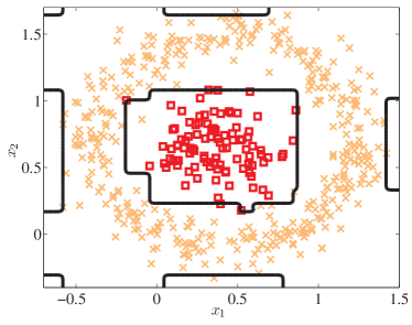
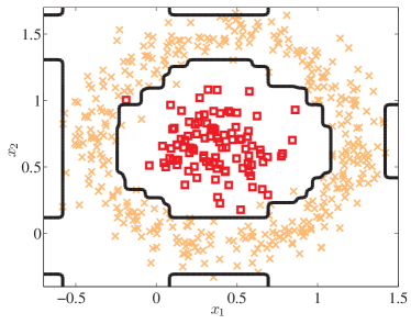
Figure 1: Decision boundaries of AdaBoost (left) and FisherBoost (right) on $2$D artificial data (positive data represented by $\square$’s and negative data by $\times$’s). Weak classifiers are decision stumps. In this case, FisherBoost intends to correctly classify more positive data in this case.

First, let us show a simple example on a synthetic dataset (more negative data than positive data) to illustrate the difference between FisherBoost and AdaBoost. Fig. 1 demonstrates the subtle difference of the classification boundaries obtained by AdaBoost and FisherBoost. We can see that FisherBoost seems to focus more on correctly classifying positive data points. This might be due to the fact that AdaBoost only optimizes the overall classification accuracy. This finding is consistent with the result in [18].

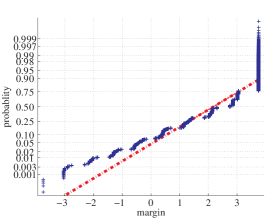
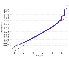
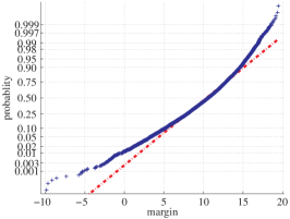
Figure 2: Normality test (normal probability plot) for the face data’s margin distribution of nodes $1$, $2$, $3$. The $3$ nodes contains $7$, $22$, $52$ weak classifiers respectively. Curves close to a straight line mean close to a Gaussian.

Face detection In this section, we compare our algorithm with other state-of-art face detectors. We first show some results about the validity of LAC (or Fisher LDA) post-processing for improving node learning in object detection. Fig. 2 illustrates the normal probability plot of margins of positive training data, for the first three nodes in the multi-exit with LAC cascade. Clearly, the larger number of weak classifiers being used, the more closely the margin follows Gaussian distribution. In other words, LAC may achieve a better performance if a larger number of weak classifiers are used. The performance could be poor with too fewer weak classifiers. The same statement applies to Fisher LDA, and LACBoost, FisherBoost, too. Therefore, we do not apply LAC/LDA in the first eight nodes because the margin distribution could be far from a Gaussian distribution. Because the late nodes of a multi-exit cascade contain more weak classifiers, we conjecture that the multi-exit cascade might meet the Gaussianity requirement better. We have compared multi-exit cascades with LDA/LAC post-processing against standard cascades with LDA/LAC post-processing in [4] and slightly improved performances were obtained.

Six methods are evaluated with the multi-exit cascade framework [10], which are AdaBoost with LAC post-processing, or LDA post-processing, AsymBoost with LAC or LDA post-processing [4], and our FisherBoost, LACBoost. We have also implemented Viola-Jones’ face detector as the baseline [2]. As in [2], five basic types of Haar-like features are calculated, which makes up of a $162,336$ dimensional over-complete feature set on an image of $24\times 24$ pixels. To speed up the weak classifier training, as in [4], we uniformly sample $10\%$ of features for training weak classifiers (decision stumps). The training data are $9,832$ mirrored $24\times 24$ face images ($5,000$ for training and $4,832$ for validation) and $7,323$ large background images, which are the same as in [4].

Multi-exit cascades with $22$ exits and $2,923$ weak classifiers are trained with various methods. For fair comparisons, we have used the same cascade structure and same number of weak classifiers for all the compared learning methods. The indexes of exits are pre-set to simplify the training procedure. For our FisherBoost and LACBoost, we have an important parameter $\theta$, which is chosen from $\{\frac{1}{10},\frac{1}{12},\frac{1}{15},$ $\frac{1}{20},\frac{1}{25},\frac{1}{30},$ $\frac{1}{40},\frac{1}{50}\}$. We have not carefully tuned this parameter using cross-validation. Instead, we train a $10$-node cascade for each candidate $\theta$, and choose the one with the best training accuracy. At each exit, negative examples misclassified by current cascade are discarded, and new negative examples are bootstrapped from the background images pool. Totally, billions of negative examples are extracted from the pool. The positive training data and validation data keep unchanged during the training process.

Our experiments are performed on a workstation with $8$ Intel Xeon E$5520$ CPUs and $32$GB RAM. It takes about $3$ hours to train the multi-exit cascade with AdaBoost or AsymBoost. For FisherBoost and LACBoost, it takes less than $4$ hours to train a complete multi-exit cascade. In other words, our EG algorithm takes less than $1$ hour for solving the primal QP problem (we need to solve a QP at each iteration). A rough estimation of the computational complexity is as follows. Suppose that the number of training examples is $m$, number of weak classifiers is $n$, At each iteration of the cascade training, the complexity for solving the primal QP using EG is $O(mn+kn^{2})$ with $k$ the iterations needed for EQ’s convergence. The complexity for training the weak classifier is $O(md)$ with $d$ the number of all Haar-feature patterns. In our experiment, $m=10,000$, $n\approx 2900$, $d=160,000$, $k<500$. So the majority of the training computation is on the weak classifier training.

We have also experimentally observed the speedup of EG against standard QP solvers. We solve the primal QP defined by (19) using EG and Mosek [17]. The QP’s size is $1,000$ variables. With the same accuracy tolerance (Mosek’s primal-dual gap is set to $10^{-7}$ and EG’s convergence tolerance is also set to $10^{-7}$), Mosek takes $1.22$ seconds and EG is $0.0541$ seconds. So EG is about $20$ times faster. Moreover, at iteration $n+1$ of training the cascade, EG can take advantage of the last iteration’s solution by starting EG from a small perturbation of the previous solution. Such a warm-start gains a $5$ to $10\times$ speedup in our experiment, while there is no off-the-shelf warm-start QP solvers available yet.

We evaluate the detection performance on the MIT+CMU frontal face test set. Two performance metrics are used here: each node and the entire cascade. The node metric is how well the classifiers meet the node learning objective. The node metric provides useful information about the capability of each method to achieve the node learning goal. The cascade metric uses the receiver operating characteristic (ROC) to compare the entire cascade’s peformance. Multiple issues have impacts on the cascade’s performance: classifiers, the cascade structure, bootstrapping etc.

We show the node comparison results in Fig. 3. The node performances between FisherBoost and LACBoost are very similar. From Fig. 3, as reported in [4], LDA or LAC post-processing can considerably reduce the false negative rates. As expected, our proposed FisherBoost and LACBoost can further reduce the false negative rates significantly. This verifies the advantage of selecting features with the node learning goal being considered.

From the ROC curves in Fig. 4, we can see that FisherBoost and LACBoost outperform all the other methods. In contrast to the results of the detection rate for each node, LACBoost is slightly worse than FisherBoost in some cases. That might be due to that many factors have impacts on the final result of detection. LAC makes the assumption of Gaussianity and symmetry data distributions, which may not hold well in the early nodes. This could explain why LACBoost does not always perform the best. Wu et al. have observed the same phenomenon that LAC post-processing does not outperform LDA post-processing in a few cases. However, we believe that for harder detection tasks, the benefits of LACBoost would be more impressive.

The error reduction results of FisherBoost and LACBoost in Fig. 4 are not as great as those in Fig. 3. This might be explained by the fact that the cascade and negative data bootstrapping remove of the error reducing effects, to some extend. We have also compared our methods with the boosted greedy sparse LDA (BGSLDA) in [18], which is considered one of the state-of-the-art. We provide the ROC curves in the supplementary package. Both of our methods outperform BGSLDA with AdaBoost/AsymBoost by about $2\%$ in the detection rate. Note that BGSLDA uses the standard cascade. So besides the benefits of our FisherBoost/LACBoost, the multi-exit cascade also brings effects.

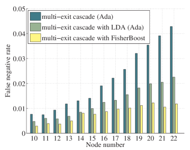
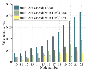
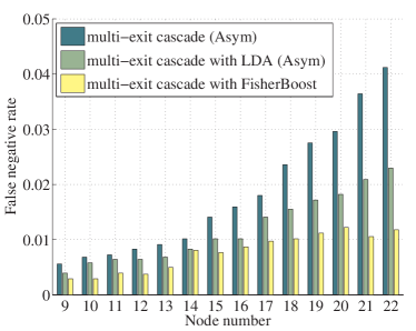
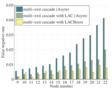
Figure 3: Node performances on the validation data. “Ada” means that features are selected using AdaBoost; “Asym” means that features are selected using AsymBoost.

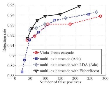
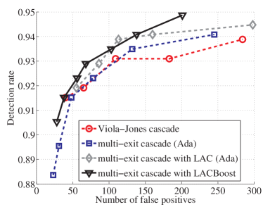
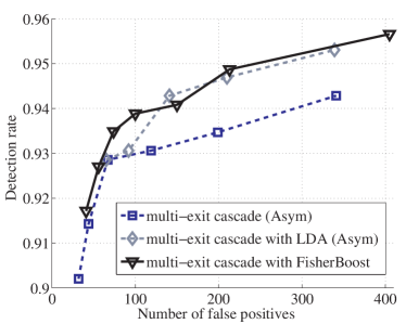
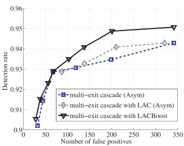
Figure 4: Cascade performances using ROC curves (number of false positives versus detection rate) on the MIT+CMU test data. “Ada” means that features are selected using AdaBoost. Viola-Jones cascade is the method in [2]. “Asym” means that features are selected using AsymBoost.

5 Conclusion

By explicitly taking into account the node learning goal in cascade classifiers, we have designed new boosting algorithms for more effective object detection. Experiments validate the superiority of our FisherBoost and LACBoost. We have also proposed to use entropic gradient to efficiently implement FisherBoost and LACBoost. The proposed algorithms are easy to implement and can be applied other asymmetric classification tasks in computer vision. We are also trying to design new asymmetric boosting algorithms by looking at those asymmetric kernel classification methods.

References

- [1] Wu, J., Mullin, M.D., Rehg, J.M.: Linear asymmetric classifier for cascade detectors. In: Proc. Int. Conf. Mach. Learn., Bonn, Germany (2005) 988–995
- [2] Viola, P., Jones, M.J.: Robust real-time face detection. Int. J. Comp. Vis. 57(2) (2004) 137–154
- [3] Viola, P., Jones, M.: Fast and robust classification using asymmetric AdaBoost and a detector cascade. In: Proc. Adv. Neural Inf. Process. Syst., MIT Press (2002) 1311–1318
- [4] Wu, J., Brubaker, S.C., Mullin, M.D., Rehg, J.M.: Fast asymmetric learning for cascade face detection. IEEE Trans. Pattern Anal. Mach. Intell. 30(3) (2008) 369–382
- [5] Demiriz, A., Bennett, K., Shawe-Taylor, J.: Linear programming boosting via column generation. Mach. Learn. 46(1-3) (2002) 225–254
- [6] Pham, M.T., Cham, T.J.: Online learning asymmetric boosted classifiers for object detection. In: Proc. IEEE Conf. Comp. Vis. Patt. Recogn., Minneapolis, MN (2007)
- [7] Wu, J., Rehg, J.M., Mullin, M.D.: Learning a rare event detection cascade by direct feature selection. In: Proc. Adv. Neural Inf. Process. Syst., Vancouver (2003) 1523–1530
- [8] Bourdev, L., Brandt, J.: Robust object detection via soft cascade. In: Proc. IEEE Conf. Comp. Vis. Patt. Recogn., San Diego, CA, US (2005) 236–243
- [9] Xiao, R., Zhu, H., Sun, H., Tang, X.: Dynamic cascades for face detection. In: Proc. IEEE Int. Conf. Comp. Vis., Rio de Janeiro, Brazil (2007)
- [10] Pham, M.T., Hoang, V.D.D., Cham, T.J.: Detection with multi-exit asymmetric boosting. In: Proc. IEEE Conf. Comp. Vis. Patt. Recogn., Anchorage, Alaska (2008)
- [11] Pham, M.T., Cham, T.J.: Fast training and selection of Haar features using statistics in boosting-based face detection. In: Proc. IEEE Int. Conf. Comp. Vis., Rio de Janeiro, Brazil (2007)
- [12] Li, S.Z., Zhang, Z.: FloatBoost learning and statistical face detection. IEEE Trans. Pattern Anal. Mach. Intell. 26(9) (2004) 1112–1123
- [13] Liu, C., Shum, H.Y.: Kullback-Leibler boosting. In: Proc. IEEE Conf. Comp. Vis. Patt. Recogn. Volume 1., Madison, Wisconsin (June 2003) 587–594
- [14] Rätsch, G., Mika, S., Schölkopf, B., Müller, K.R.: Constructing boosting algorithms from SVMs: An application to one-class classification. IEEE Trans. Pattern Anal. Mach. Intell. 24(9) (2002) 1184–1199
- [15] Beck, A., Teboulle, M.: Mirror descent and nonlinear projected subgradient methods for convex optimization. Oper. Res. Lett. 31(3) (2003) 167–175
- [16] Collins, M., Globerson, A., Koo, T., Carreras, X., Bartlett, P.L.: Exponentiated gradient algorithms for conditional random fields and max-margin Markov networks. J. Mach. Learn. Res. (2008) 1775–1822
- [17] MOSEK ApS: The MOSEK optimization toolbox for matlab manual, version 5.0, revision 93 (2008) http://www.mosek.com/.
- [18] Paisitkriangkrai, S., Shen, C., Zhang, J.: Efficiently training a better visual detector with sparse Eigenvectors. In: Proc. IEEE Conf. Comp. Vis. Patt. Recogn., Miami, Florida, US (June 2009)