Time Evolution of the Spread of Diseases with a General Infectivity Profile on a Complex Dynamic Network

Abstract

This manuscript introduces a new analytical approach for studying the time evolution of disease spread on a finite size network. Our methodology can accommodate any disease with a general infectivity profile. This new approach is able to incorporate the impact of a general intervention - at the population level - in a number of different ways. Below, we discuss the details of the equations involved and compare the outcomes of analytical calculation against simulation results. We conclude with a discussion of possible extensions of this methodology.

1 Introduction

The time evolution of disease spread within human populations is a very interesting and multifaceted topic; it is closely related to the rate of new infections in a population, which has significant implications when designing public health policy. The spread of disease within a population is complex and depends on a number of different factors, including, social connectivity patterns, cultural practices and education surrounding hygiene and intervention strategies, the level of preexisting immunity and finally, the infectivity of the infectious agent. In order to produce a reliable estimate of the new infection rate, a model should incorporate - at the very least - the abovementioned factors.

The spread of disease in a population involves a complex stochastic branching process. This process is comprised of three distinct constituents, namely, the stochastic phase, exponential phase and declining phase. To date, each phase has undergone a considerable amount of scrutiny using two main techniques, i.e., compartmental and network models. The stochastic phase was studied using discrete and continuous time approaches [1, 2, 3, 4], while the exponential and declining phases were studied using a variety of models and techniques, including, compartmental [5, 6, 7] and network models [2, 3, 4, 8, 9]. Both of these method, however, have their downfalls; that is, compartmental models deal solely with constant infection and removal rates, do not incorporate any memory of infections, distribute the force of infection uniformly in the population, and include the finite size effect in a very simple manner. Moreover, some of the limitations associated with network methods are seen in the work by Nel et.al [2] and Davoudi et.al [9]. They considered disease transmission to follow the generation time concept, that is, they assumed infection or recovery/removal occurred at a discrete time within the period of $\tau$. This led to a significant simplification of the calculations, thus, the model became unrealistic for a disease with a long period of infection. The work by Volz et.al [8] included the finite size effect in a comprehensive manner, but the method could not accommodate diseases with a complex infection profile. To circumvent these downfalls we present a new methodology which can sustain complex infection and recovery/removal profiles, and can take the finite size effect into account, in a precise manner.

Below, we first discuss the required theoretical components for this methodology. We then compare theoretical results against simulation results to understand the precision of the method and the level of approximation involved. Subsequently, we discuss the possibility of extending this current methodology to address systems with a complex dynamic network structure.

2 Theory

2.1 Basic Notions

We consider the preexisting contact network to be the platform for disease transmission within a population. Individuals are represented by a vertex and contact between two individuals is represented by a link. Links are composed of two stubs, each of which is attached to its own vertex. For a population of size $N$, we create a random network where the degree of connectivity between vertices is coded by the probability distribution function, $p_{k}$, where $k$ is the degree. The average excess degree[2] is defined as the degree of secondarily infected vertices and is given by $Z_{x}=z_{2}/z_{1}$ where $z_{1}=\langle k\rangle_{p_{k}}$ is the average degree, $z_{2}=\langle k^{2}\rangle_{p_{k}}-\langle k\rangle_{p_{k}}$ and finally $\langle k^{n}\rangle_{p_{k}}=\sum_{\kappa=0}^{\infty}k^{n}p_{\kappa}$.

The process of disease transmission within a population is a complex phenomenon. Individuals, or vertices, are infected and removed at specific times, denoted by $t_{i}$ and $t_{r}$ respectively. Infected vertices are removed from the population for a number of reasons, including death, quarantine, and recovery for example. Moreover, the age of infection and the time between infection and removal, or the “time-to-removal”,for each infected vertex are defined as $\tau=t-t_{i}$ and $\tau_{r}=t_{r}-t_{i}$, respectively. The transmission of infection between an infected vertex and a susceptible vertex is dictated by the infectivity function, $\lambda_{i}(\tau)$, in which $\lambda_{i}(\tau)d\tau$ denotes the probability of transmission during the interval $\tau$ and $\tau+d\tau$. In the same manner, we define the removal function as $\lambda_{r}(\tau)$, in which $\lambda_{r}(\tau)d\tau$ yields the chance of removal of an infected vertex during the interval $\tau$ and $\tau+d\tau$. The transmissibility, $T(\tau,\tau_{r})$, provides the probability of transmission until time $\tau$, for an infected vertex that is removed after time $\tau_{r}$ and satisfies the following equation[10, 11]

$$T(\tau,\tau_{r})=\left\{\begin{array}[]{ccc}1-\exp\left(-\int_{0}^{\tau}\lambda_{i}(u)du\right)&&\tau<\tau_{r}\\ \\ 1-\exp\left(-\int_{0}^{\tau_{R}}\lambda_{i}(u)du\right)&&{otherwise}\end{array}\right.$$ (1)

We define $\Psi(\tau_{r})$[10] as the probability that a vertex has a time-to-removal $\geq\tau_{r}$, which is given by

$$\Psi(\tau_{r})=\exp\left(-\int_{0}^{\tau_{R}}\lambda_{r}(u)du\right),$$ (2)

subject to the condition $\Psi(\infty)=0$. We also define the probability density function as $\psi(\tau_{r})=-\frac{d\Psi(\tau_{r})}{d\tau_{r}}$ (or $\Psi(\tau_{r})=\int_{\tau_{r}}^{\infty}\psi(u)du$). The basic reproduction number is given by ${\cal R}_{0}=\frac{z_{2}}{z_{1}}T$, where $T$ is the ultimate transmissibility $T=\int_{0}^{\infty}\psi(\tau)T(\tau,\tau<\tau_{r})$[3].

Finally, $J(t)$ denotes the rate of newly infected vertices at time $t$. At a given time $t$, a fraction, $\Psi(\tau)$, of infected vertices $J(t-\tau)$ with the age of infection $\tau$ remain infectious. Therefore, the total number of infectious vertices, at a given time, can be calculated by

$$N_{i}(t)=\int_{0}^{t}J(t-\tau)\Psi(\tau)d\tau$$ (3)

and the number of removed and susceptible vertices are given by

$$N_{r}(t)=\int_{0}^{t}J(t-\tau)\left[1-\Psi(\tau)\right]d\tau,$$ (4)

and

$$N_{s}(t)=N-N_{r}(t)-N_{i}(t).$$ (5)

respectively.

2.2 Disease Transmission Dynamics on a Network

In the following section we introduce and discuss the set of equations we use to find the rate of new infections $J(t)$ as a function of time. This calculation becomes possible once we combine the network aspects (vertices connectivity) with the disease status of each vertex. To elaborate, we start with one infectious vertex with excess degree $Z_{x}$, and assume that it was infected at time $t_{i}=0$. With this knowledge, we then calculate the number of new infection that arose from this infected vertex, at the later time $t=\tau$, using

$$J(\tau)=\Psi(\tau)\frac{dT(\tau,\tau<\tau_{r})}{d\tau}Z_{x},$$ (6)

where $\frac{dT(\tau,\tau<\tau_{r})}{d\tau}$ is the contribution of each link to disease transmission between time $\tau$ and $\tau+d\tau$, given that the vertex was not removed by time $t$; the resulting contribution of $Z_{x}$ link is given by $\frac{dT(\tau,\tau<\tau_{r})}{d\tau}Z_{x}$. The equation above is then multiplied by $\Psi(\tau)$ in order to take the chance of removal into account. The total number of infections caused by the first infected vertex is given by $TZ_{x}$ where $T=\int_{0}^{\infty}\Psi(\tau)\frac{dT(\tau,\tau<\tau_{r})}{d\tau}d\tau=\int_{0}^{\infty}\psi(\tau)T(\tau,\tau<\tau_{r})d\tau$ is the ultimate transmissibility, which yields the probability of infection along a link.

Equation (6) can be easily extended to the initial phase of an epidemic, assuming that the excess degree of all vertices is the same. In general, the renewal equation for $J(t)$ is as follows[12, 3]

$$J(t)=\int_{0}^{t}J(t-\tau)\Psi(\tau)\frac{dT(\tau,\tau<\tau_{r})}{d\tau}Z_{x}(t,\tau)d\tau$$ (7)

The right hand side of the above equation gives the total number of transmitting links $\lambda(t)$ at time $t$, which leads to $J(t)\approx\lambda(t)$ infections[9]. Equation (7), where $Z_{x}(t,\tau)\approx Z_{x}=z_{2}/z_{1}$, can be used before the finite size effect becomes important, which is a valid assumption while $N_{r}(t)+N_{i}(t)\ll N_{s}(t)$. In the limit $N_{r}(t)+N_{i}(t)\sim N_{s}(t)$ , only a fraction of $Z_{x}$ is used to connect the infected and susceptible vertices. An appropriate approximation for $Z_{x}(t,\tau)$ is given below.

$Z_{x}(t,\tau)$ is calculated in two steps. First, the typical degree of infected vertices is calculated during the process of disease transmission. Second, an estimate of the average number of links an infected vertex - with an infectious period of $\tau$ - could have with susceptible vertices, at time $t$, is made.

The first step is easily preformed for a random network [2, 9]. A vertex is randomly picked and assigned to a collected class, while the probability that the chosen vertex has the degree $k$ is given by $q_{k}(1)=p_{k}$. The function argument shows the number of collected vertices. The degree distribution of the uncollected vertices is given by $p_{k}(1)=p_{k}$. The expected degree of the first collected vertex is $\tilde{z}(1)=z_{1}$ and the average degree of the uncollected vertices is $z(1)=z_{1}$. A second vertex is then chosen by picking a random stub. The probability that the second vertex has degree $k$ is given by $q_{k}(2)=kp_{k}/z(1)$, the degree distribution of the collected vertices is calculated as follows $\tilde{p}_{k}(2)=(q_{k}(1)+q_{k}(2))/2$ and the degree distribution of the uncollected vertices is specified by $p_{k}(2)=(Np_{k}-2\tilde{p}_{k}(2))/(N-2)$. The probability that the $nth$ chosen vertex has degree $k$ is $q_{k}(n)=kp_{k}(n-1)/z(n-1)$ and, in the same manner, the degree distributions of collected and uncollected vertices are given by

$$\tilde{p}_{k}(n) =\sum_{i=1}^{n}q_{k}(n)/n,$$ (8)

$$p_{k}(n) =(Np_{k}-n\tilde{p}_{k}(n))/(N-n),$$ (9)

where $z(n)=\sum_{i=0}^{\infty}kp_{k}(n)$ is the average degree of uncollected vertices after $n$ collections. We define $\tilde{z}(n)=\sum_{i=0}^{\infty}k\tilde{p}_{k}(n)$ as the average degree of collected vertices after $n$ collections. The latter equations take the following form in the continuous limit

$$\frac{d\tilde{p}_{k}(n)}{dn} =\frac{p_{k}(n)}{n}\left(\frac{k}{z(n)}-1\right),$$ (10)

$$\frac{dp_{k}(n)}{dn} =\frac{p_{k}(n)}{N-n}\left(1-\frac{k}{z(n)}\right).$$ (11)

The average degree of infected vertices that are infected between time $t$ and $t+dt$ is given by

$$z_{j}(t) =\frac{[N_{r}(t)+N_{i}(t)+J(t)dt]\tilde{z}(N_{r}(t)+N_{i}(t)+J(t)dt)-(N_{r}(t)+N_{i}(t))\tilde{z}(N_{r}(t)+N_{i}(t))}{J(t)dt}$$ (12)

$$=\tilde{z}(N_{r}(t)+N_{i}(t))+[N_{r}(t)+N_{i}(t)]\left.\frac{d\tilde{z}(n)}{dn}\right|_{n=N_{r}(t)+N_{i}(t)}.$$ (13)

In the same manner, we find that the average degree of removed $z_{r}(t)$, infectious $z_{i}(t)$, and susceptible classes $z_{s}(t)$ with the following formulas, respectively

$$z_{r}(t) =\tilde{z}(N_{r}(t)),$$ (14)

$$z_{i}(t) =\frac{[N_{r}(t)+N_{i}(t)]\tilde{z}(N_{r}(t)+N_{i}(t))-N_{r}(t)\tilde{z}(N_{r}(t))}{N_{i}(t)},$$ (15)

$$z_{s}(t) =z(N_{s}(t)),$$ (16)

$Z_{x}(t,\tau)$ can now be easily estimated. The number of stubs belonging to infected vertices, between time $t-\tau$ and $t-\tau+d\tau$, is given by $z_{j}(t-\tau)J(t-\tau)d\tau$. The probability of one of these stubs connecting to the stub of a susceptible vertex, at time $t$, is given by $z_{s}(t)N_{s}(t)/z_{1}N$, and thus

$$Z_{x}(t,\tau)\approx z_{j}(t-\tau)\frac{z_{s}(t)N_{s}(t)}{z_{1}N}.$$ (17)

We also considered other approximation with different renewal equations

$$J(t)=\int_{0}^{t}J(t-\tau)\Psi(\tau)\frac{dT(\tau,\tau<\tau_{r})}{d\tau}Z_{x}N_{s}(t)/Nd\tau,$$ (18)

This new methodology provides a solution for SIR compartmental models, whereby the force of infection, $\beta(\tau)$, and recovery rate, $\gamma(\tau)$, are functions of $\tau$ [4]. This is equivalent to the approximation $Z_{x}(t,\tau)\approx Z_{x}N_{s}(t)/N$.

3 Numerical results for the most simplistic network

In this section we present the numerical result for three stylized networks, namely binomial $p_{k}=\binom{N}{k}p^{k}(1-p)^{N-k}$ with $p=z_{1}/(N-1)$ ($z_{1}=10$), exponential $p_{k}=(1-\exp(-1/\kappa))\exp(-k/\kappa)$ ($\kappa=10$) and bimodal, which are depicted in figure 1. The size of the networks were $N=10,000$. To obtain a numerical solution with the current methodology, we first created two sequences, namely $z(n)$ and $\tilde{z}(n)$, for a specific network using equation (8) and (9). We then recursively used the renewal equation (7) to obtain the number of infections at a later time, meanwhile $z_{j}(t)$, $z_{s}(t)$ and $Z_{x}(t,\tau)$ were calculated.

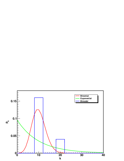
Figure 1: Three different degree distributions, binomial $z_{1}=10$, exponential $\kappa=10$ and bimodal network.

In figure 2, we compare the number of removed vertices for the new calculation (Analytical-N) and the compartmental model (Analytical-C), against simulations for a binomial network. Top left panel $z_{1}=10$, $\lambda_{i}=0.35$ and $\lambda_{r}=2$; top right panel $\lambda_{i}=0.2$ and $\lambda_{r}=1$; bottom left panel $\lambda_{i}=0.5$ and $\lambda_{r}=2$; and bottom right panel $\lambda_{i}=0.3$ and $\lambda_{r}=1$. Both analytical approaches performed well for the binomial network, within this range of parameter values. The current approach slightly overestimated the final size for small ${\cal R}_{0}$ values and slightly underestimated the final size for large ${\cal R}_{0}$ values.

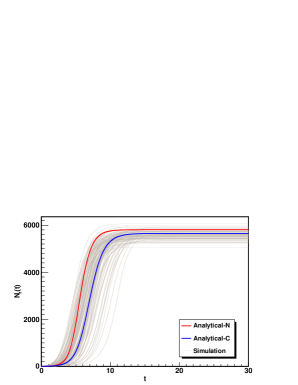
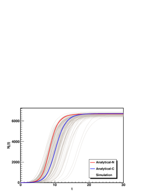
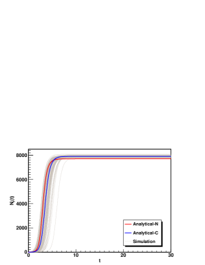
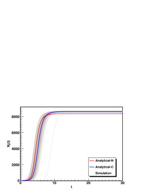
Figure 2: $z_{1}=10$, $\lambda_{i}=0.25$ and $\lambda_{r}=2$ left top panel, $\lambda_{i}=0.2$ and $\lambda_{r}=1$ right top panel, $\lambda_{i}=0.5$ and $\lambda_{r}=2$ left bottom panel, and finally $\lambda_{i}=0.3$ and $\lambda_{r}=1$ right bottom panel.

In figure 3, we compare the number of removed vertices for the new calculation (Analytical-N) and compartmental model (Analytical-C), against simulations for exponential network. Top left panel $\kappa=10$, $\lambda_{i}=0.35$ and $\lambda_{r}=2$; top right panel $\lambda_{i}=0.2$ and $\lambda_{r}=1$; bottom left panel $\lambda_{i}=0.5$ and $\lambda_{r}=2$; and, bottom right panel $\lambda_{i}=0.3$ and $\lambda_{r}=1$. The compartmental model was inferior to thebinomial network; for exponential networks, as we expect that $Z_{x}(t,\tau)\approx Z_{x}$ will become a poor predictor for any network with a very wide degree distribution.

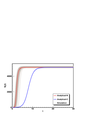
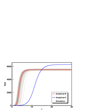
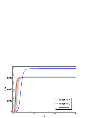
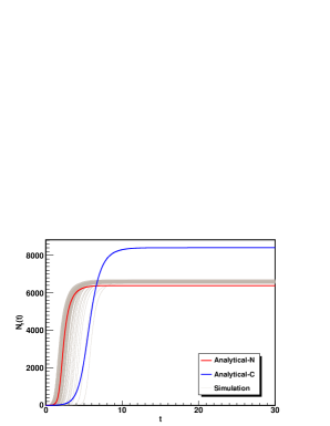
Figure 3: $\kappa=10$, $\lambda_{i}=0.25$ and $\lambda_{r}=2$ left top panel, $\lambda_{i}=0.2$ and $\lambda_{r}=1$ right top panel, $\lambda_{i}=0.5$ and $\lambda_{r}=2$ left bottom panel, and finally $\lambda_{i}=0.3$ and $\lambda_{r}=1$ right bottom panel.

Finally in figure 4, we compare the number of removed vertices for the new calculation (Analytical-N) and compartmental model (Analytical-C), versus simulations for bimodal network. Top left panel $\lambda_{i}=0.25$ and $\lambda_{r}=2$; top right panel $\lambda_{i}=0.2$ and $\lambda_{r}=1$; bottom left panel $\lambda_{i}=0.5$ and $\lambda_{r}=2$; and, bottom right panel $\lambda_{i}=0.3$ and $\lambda_{r}=1$.

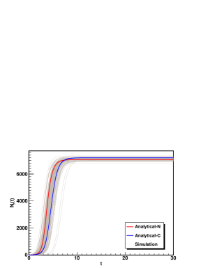
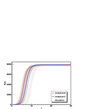
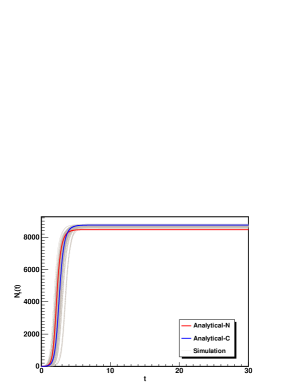
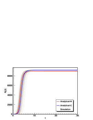
Figure 4: $\lambda_{i}=0.25$ and $\lambda_{r}=2$ left top panel, $\lambda_{i}=0.2$ and $\lambda_{r}=1$ right top panel, $\lambda_{i}=0.5$ and $\lambda_{r}=2$ left bottom panel, and finally $\lambda_{i}=0.3$ and $\lambda_{r}=1$ right bottom panel.

The small deviation for the current formalism and simulation for low and high ${\cal R}_{0}$ values is due to overestimating/underestimating the number of infections from the number of transmitting links.

The compartmental model fails to correctly capture the dynamics of the epidemics for populations in which a sizable portion of individuals have low degree, which turns to be an important characteristic of realistic human contact networks.

4 Extensions

In this section, we discuss different extensions of the methodology to address other models such as, open system models (in which the number of vertices is a function of time), dynamic network models, susceptible-infectious-removed-susceptible SIRS models, and multi-type systems (including systems with different age groups, each of which having different connectivity, infectivity, susceptibility, etc).

4.1 Multi-type system

Here we consider a system consisting of more than one type of nodes,where each node type has different inter- and intra- degree distributions, transmissibilities, and removal distributions. We define a set of node types and index them with superscript $\alpha$. We first define $N^{\alpha}$, $\lambda_{r}^{\alpha\beta}(\tau)$, $\lambda_{i}^{\alpha\beta}(\tau)$ and $p_{k}^{\alpha}$ as the number of vertices , new removal function, infectivity function and degree distribution of type $\alpha$, respectively. We also define $N_{\alpha}^{\beta}(t)$ as the number of vertices from type $\beta$ in the classes $\alpha$. Here we assume the connectivity between vertices, in different node types, is completely random. The current method can be further extended if there is any preference for intra- or inter-connectivity between vertices in different types.

Our renewal equation(7) takes the following trivial form

$$J^{\alpha}(t)=\sum_{\beta}\int_{0}^{t}J^{\beta}(t-\tau)\Psi^{\beta}(\tau)\frac{dT^{\beta\alpha}(\tau,\tau<\tau_{r})}{d\tau}Z_{x}^{\beta\alpha}(t,\tau)d\tau$$ (19)

$Z_{x}^{\beta\alpha}$, however, is now a more complex function and must be calculated using the following steps; first, the collected and uncollected degree distribution for each type must be found. To do so we randomly pick a vertex. The probability that the first chosen vertex is in type $\alpha$ is $n^{\alpha}(1)=N^{\alpha}/N$, as a result the probability that the chosen vertex has degree $k$ and comes from type $\alpha$ is given by $q_{k}^{\alpha}(1)=n^{\alpha}(1)p_{k}^{\alpha}$. The degree distributions of collected and uncollected classes are given by $\tilde{p}_{k}^{\alpha}(1)=q_{k}^{\alpha}(1)$ and $p_{k}^{\alpha}(1)=(N^{\alpha}p_{k}^{\alpha}-n^{\alpha}(1)\tilde{p}_{k}^{\alpha}(1))/(N-n^{\alpha}(1))$. Now the second vertex can be randomly chosen by selecting a random stub. The probability that the second vertex has degree $k$ and belongs to type $\alpha$ is given by $q_{k}^{\alpha}(2)=n^{\alpha}(2)kp_{k}^{\alpha}(2)/z^{\alpha}(1)$ where $n^{\alpha}(2)=(N^{\alpha}-n^{\alpha}(1))/(N-1)$ and $z^{\alpha}(1)=\sum_{k}kp_{k}^{\alpha}(1)$. The degree distribution of collected and uncollected classes are given by $\tilde{p}_{k}^{\alpha}(2)=(q_{k}^{\alpha}(1)+q_{k}^{\alpha}(2))/(n^{\alpha}(1)+n^{\alpha}(2))$ and $p_{k}^{\alpha}(2)=(N^{\alpha}p_{k}^{\alpha}-(n^{\alpha}(1)+n^{\alpha}(2))\tilde{p}_{k}^{\alpha}(2))/(N-n^{\alpha}(1)-n^{\alpha}(2))$. It is thus plausible that the $nth$ chosen vertex is in type $\alpha$ and has degree $k$ with the probability $q_{k}^{\alpha}(n)=n^{\alpha}(n)kp_{k}^{\alpha}(n-1)/z^{\alpha}(n-1)$. In the same manner

$$\tilde{p}_{k}^{\alpha}(n) =\frac{\sum_{i=1}^{n}q_{k}^{\alpha}(i)}{\sum_{i=1}^{n}n^{\alpha}(i)},$$ (20)

$$p_{k}^{\alpha}(n) =\frac{N^{\alpha}p_{k}^{\alpha}-\sum_{i=1}^{n}n^{\alpha}(i)\tilde{p}_{k}^{\alpha}(n)}{N-\sum_{i=1}^{n}n^{\alpha}(i)}.$$ (21)

Therefore, $z_{j}^{\alpha}(t)$, $z_{r}^{\alpha}(t)$, $z_{i}^{\alpha}(t)$, and $z_{s}^{\alpha}(t)$ are given by

$$z_{j}^{\alpha}(t) =\tilde{z}^{\alpha}(N_{r}^{\alpha}(t)+N_{i}^{\alpha}(t))+[N_{r}^{\alpha}(t)+N_{i}^{\alpha}(t)]\left.\frac{d\tilde{z}^{\alpha}(n)}{dn}\right|_{n=N_{r}^{\alpha}(t)+N_{i}^{\alpha}(t)},$$ (22)

$$z_{r}^{\alpha}(t) =\tilde{z}^{\alpha}(N_{r}^{\alpha}(t)),$$ (23)

$$z_{i}^{\alpha}(t) =\frac{[N_{r}^{\alpha}(t)+N_{i}^{\alpha}(t)]\tilde{z}^{\alpha}(N_{r}^{\alpha}(t)+N_{i}^{\alpha}(t))-N_{r}^{\alpha}(t)\tilde{z}(N_{r}^{\alpha}(t))}{N_{i}^{\alpha}(t)},$$ (24)

$$z_{s}^{\alpha}(t) =z^{\alpha}(N_{s}^{\alpha}(t)),$$ (25)

where $N_{i}^{\alpha}(t)=\int_{0}^{t}J^{\alpha}(t-\tau)\Psi^{\alpha}(\tau)d\tau$, $N_{r}^{\alpha}(t)=\int_{0}^{t}J^{\alpha}(t-\tau)\left[1-\Psi^{\alpha}(\tau)\right]d\tau$ and $N_{s}^{\alpha}(t)=N-N_{i}^{\alpha}(t)-N_{r}^{\alpha}(t)$. Finally, we have

$$Z_{x}^{\alpha\beta}(t,\tau)\approx z_{j}^{\alpha}(t-\tau)\frac{z_{s}^{\beta}(t)N_{s}^{\beta}(t)}{z_{1}N}.$$ (26)

As an example, we study an exponential degree distribution with $\kappa=10$, $\lambda_{i}=0.2$ and $\lambda_{r}=1$. We use the multi-type framework to show how easily one can replicate the results obtained earlier for the similar degree distribution in section{……} the current formalism. We devide the network to groups of vertices, each of which has a specifc degree where $\{\alpha,\;\beta\}=\{k,\;k^{\prime}\}$. Our multi-type renewal equations is given by

$$J^{\alpha}(t)=\int_{0}^{t}\Psi(\tau)\frac{dT(\tau,\tau<\tau_{r})}{d\tau}\sum_{\beta}J^{\beta}(t-\tau)Z_{x}^{\beta\alpha}\frac{N_{s}^{\alpha}(t)}{N^{\alpha}}d\tau$$ (27)

A crude approximation for the contact matrix, ${\cal Z}_{x}$, is described below. The probability of a stub from a node type $\alpha$ connecting to a stub from node type $\beta$ is given by $N^{\beta}z_{1}^{\beta}/Nz_{1}$. This implies that the total number of links going from type $\alpha$ to $\beta$ can be approximated by $N^{\alpha}z_{1}^{\alpha}N^{\beta}z_{1}^{\beta}/Nz_{1}$ and consequently the number links per vertex is given by $z_{1}^{\alpha}N^{\beta}z_{1}^{\beta}/Nz_{1}$.

In figure 5 we compare the result of the current calculation (Analytical-N) against one type (Analytical-C1), multi-type (Analytical-Cn) and simulation models for the above-mentioned network, whereby $\lambda_{i}=0.2$ and $\lambda_{r}=1$. The excellent agreement between the two methods demonstrates that a network with a general degree distribution can be examined as a set multi-type system, within the current approximation. Both the multi-type framework and the current formalism, as discussed in section3, yield similar levels of error when predicting the epidemic curve. Thus, one can use either approach; however, the multitype approach may become very expensive computationally for a network with a very wide degree distribution.

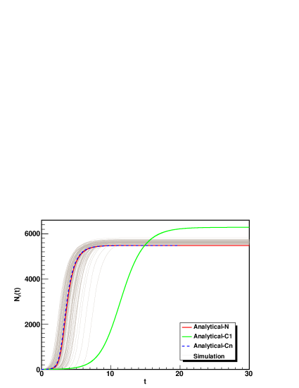
Figure 5: $\kappa=10$, $\lambda_{i}=0.2$ and $\lambda_{r}=1$.

4.2 Open system

In an open system, the number of vertices is a function of time. The previous set of equations still hold for an open system, however, we must now keep track of entering and exiting vertices in each class, as well as the corresponding change in degree distribution. For example, the number of vertices in a susceptible class can be calculated from

$$\frac{dN_{s}(t)}{dt}=\sum_{k}(\Pi_{in,s}(k,t)-\Pi_{out,s}(k,t)),$$ (28)

where $\Pi_{in/out,s}(k,t)$ is the rate of entry/exit of susceptible vertices with degree $k$ at time $t$. The degree distribution of collected and uncollected vertices can be calculated from

$$\frac{d\tilde{p}_{k}(n,t)}{dt} =\frac{\partial\tilde{p}_{k}(n,t)}{\partial n}\frac{dn}{dt}+\frac{\Pi_{in,ir}(k,t)-\Pi_{out,ir}(k,t)}{n(t)},$$ (29)

$$\frac{dp_{k}(n,t)}{dt} =\frac{\partial p_{k}(n,t)}{\partial n}\frac{dn}{dt}+\frac{\Pi_{in,s}(k,t)-\Pi_{out,s}(k,t)}{N(t)-n(t)},$$ (30)

where $\Pi_{in,ir}(k,t)=\Pi_{in,i}(k,t)=\Pi_{in,r}(k,t)$. The first term on the right hand side of both equations is the contribution of collecting vertices, the second term arises from vertices entering or exiting the network. The partial derivatives of both equations are calculated from (10) and (11) respectively

$$\frac{\partial\tilde{p}_{k}(n,t)}{\partial t} =\frac{p_{k}(n(t),t)}{n(t)}\left(\frac{k}{z(n(t))}-1\right),$$ (31)

$$\frac{\partial p_{k}(n,t)}{\partial t} =\frac{p_{k}(n(t),t)}{N(t)-n(t)}\left(1-\frac{k}{z(n(t))}\right).$$ (32)

4.3 Dynamic network

As another possible extension, we consider networks where the degree of each vertex is a function of time. Dynamic networks are a simple example of an open system with the constrains

$$\sum_{k}\Pi_{in,\alpha}(k,t)=\sum_{k}\Pi_{out,\alpha}(k,t)$$ (33)

where $\alpha=\{s,\;i,\;r\}$ is an index for susceptible, infectious and removed vertices. Accordingly, the outflow of vertices with a specific degree from a given class should be replaced by the same number of vertices but with different degrees. This is a consequent of the fact that infection is instantaneous and that a removed vertex remains removed. $\Pi_{in/out,\alpha}(k,t)$ could have complex dynamics as long as the above constraints are satisfied.

4.4 SIRS model

For the SIRS model, we first need to introduce the probability function, which specifies the chance of re-infection over time, once the infected vertex has recovered. This variable is generally a function of time and can be measured with respect to any infection time reference. We define the susceptibility function, $\lambda_{s}(\tau)$, in which $\lambda_{s}(\tau)d\tau$ gives the probability of an infected vertex becoming susceptible again in the interval $\tau$ and $\tau+d\tau$. We define $\Psi_{\alpha\beta}(\tau_{s})$ as a probability function which give the probability of the time of movement from disease state $\alpha$ to $\beta$, moreover

$$\Psi_{\alpha\beta}(\tau_{s})=\exp\left(-\int_{0}^{\tau_{r}}\lambda_{\alpha\beta}(u)du\right)$$ (34)

The number of susceptible and removed vertices is given by

$$N_{s}(t) =N-\int_{0}^{t}J(t-\tau)d\tau+\int_{0}^{t}J(t-\tau)[1-\Psi_{rs}(\tau)]d\tau,$$ (35)

$$N_{r}(t) =\int_{0}^{t}J(t-\tau)[1-\Psi_{ir}(\tau)]d\tau-\int_{0}^{t}J(t-\tau)[1-\Psi_{rs}(\tau)]d\tau$$

$$=\int_{0}^{t}J(t-\tau)[\Psi_{rs}(\tau)-\Psi_{ir}(\tau)]d\tau.$$ (36)

The degree distribution of collected and uncollected vertices is calculated as follows

$$\frac{d\tilde{p}_{k}(n,t)}{dt} =\frac{\partial\tilde{p}_{k}(n,t)}{\partial n}\frac{dn}{dt}-\frac{\Pi_{out,r}(k,t)}{n(t)},$$ (37)

$$\frac{dp_{k}(n,t)}{dt} =\frac{\partial p_{k}(n,t)}{\partial n}\frac{dn}{dt}+\frac{\Pi_{in,s}(k,t)}{N(t)-n(t)},$$ (38)

where $\Pi_{out,r}(k,t)$ is the outflow of recovered vertices to susceptible classes and in the same manner $\Pi_{in,s}(k,t)$ is inflow of susceptible vertices from the recovered class; this calculation involves defining the rate of outgoing recovered vertices as

$$J_{out}(t)=\frac{d}{dt}\int_{0}^{t}J(t-\tau)(1-\Psi_{rs}(\tau))d\tau.$$ (39)

We also define the rate of outgoing degree of recovered vertices as

$$z_{out}(t)=\frac{d}{dt}\int_{0}^{t}J(t-\tau)z_{j}(t-\tau)(1-\Psi_{rs}(\tau))d\tau.$$ (40)

The expected degree of outgoing recovered vertices is then given by

$$k_{out}(t)=\frac{\zeta_{out}(t)}{J_{out}(t)},$$ (41)

and as a result

$$\Pi_{out,r}(k,t)=\Pi_{in,s}(k,t)=\delta_{k,k_{out}(t)}J_{out}(t).$$ (42)

In practice $k_{out}(t)$ is not an integer function since it gives the average degree of new susceptible vertices; thus, one must properly distribute new vertices around $k_{out}(t)$ to ensure that the average degree of the system remains constant.

5 Conclusions and Discussion

The novel methodology outlined above allows us to evaluate the time evolution of disease spread on a network. Our methodology is able to accommodate diseases with very general infectivity profiles. Additionally, this methodology can manage multi-type networks, dynamical networks, and SIRS systems. The precision of this methodology depends on the accuracy of the kernel of the renewal equation for the infection rate, which will be the subject of future investigations.

6 Acknoledgment

BP would like to acknowledge the support of the Canadian Institutes of Health Research (grant nos. MOP-81273, PPR-79231 and PTL-97126 [Team Leader grant (CanPan II)]) and the Michael Smith Foundation for Health Research (Senior Scholar Funds). BD was supported by these grants.

References

- [1] M. Marder, Phys. Rev. E 75, 066103 (2007).
- [2] P.-A. Noel, B. Davoudi, L. J. Dub, R. C. Brunham and B. Pourbohloul, Phys. Rev. E 79, 026101 (2008).
- [3] B. Davoudi, J. C. Miller, R. Meza, L. A. Meyers, D. J. D. Earn, B. Pourbohloul, Submitted to Jour. Theo. Bio.
- [4] J. C. Miller, B. Davoudi, R. Meza, A. C. Slim, B. Pourbohloul, Jour. Math. Bio., 262, 107 (2010).
- [5] N. T. J Bailey, The Mathematical Theory of Infection Disease and its applications (Hafner Press, New York, 1975).
- [6] R. M. Anderson and R. M. May, Infectious Disease of Humans (Oxford University Press, Oxford, 1991).
- [7] F. Brauer, P. van den Driessche and J. Wu, Mathematical Epidemiology (Lecture Notes in Mathematics, Mathematical Biosciences subseries 1945, Springer, 2008).
- [8] E. Volz, arXiv:0705.2092v1; E. Volz and L. A. Meyers, arXiv:070521v1.
- [9] B. Davoudi, F. Brauer, B. Pourbohloul, submitted.
- [10] D. R. Cox and D. Oakes, Analysis of survival data (Chapman & Hall 1984).
- [11] M. E. J. Newman, Phys. Rev. E 66, 016128 (2002).
- [12] A. J. Lotka, Ann. of Math. Stat. 10, 1 (1939).