Abstract

Symmetric informationally complete positive operator valued measures (SIC-POVMs) are studied within the framework of the probability representation of quantum mechanics. A SIC-POVM is shown to be a special case of the probability representation. The problem of SIC-POVM existence is formulated in terms of symbols of operators associated with a star-product quantization scheme. We show that SIC-POVMs (if they do exist) must obey general rules of the star product, and, starting from this fact, we derive new relations on SIC-projectors. The case of qubits is considered in detail, in particular, the relation between the SIC probability representation and other probability representations is established, the connection with mutually unbiased bases is discussed, and comments to the Lie algebraic structure of SIC-POVMs are presented.

Keywords: SIC-POVM, probability representation of quantum mechanics, star-product-quantization scheme, quantum tomography, Lie algebraic structure.

1 Introduction

The properties of light beams in fibers [1, 2, 3], analytic signals [4, 5], and quantum systems [6, 7, 8, 9, 10] are extensively studied, in particular, within the framework of tomographic-probability representation.

The probability representation of quantum mechanics was introduced recently in [11, 12]. According to this representation, the notion of wave function [13] and density matrix [14, 15] can be replaced by the notion of a fair probability distribution which determines the quantum state. Indeed, the density operator (and all its other phase-space representations like the Wigner function [16], Husimi $Q$-function [17], and Sudarshan–Glauber $P$-function [18, 19] for continuous degrees of freedom) is related to the probability distribution with an integral transform like the Radon transform [20] (see also [21]).

The probability representation is constructed also for discrete spin variables [22, 23] and developed in [24, 25, 26] (see also the recent review [27]). From this point of view, the probability representation of quantum mechanics is completely equivalent to the other ones. On the other hand, this representation has some new and unexpected aspects, for instance, quantum states and transitions between them are described by positive probabilities and positive transition probabilities, respectively, instead of complex wave functions and complex transition amplitudes inherent in the conventional formulation of quantum mechanics. Thus, one can say that, in the probability representation, the picture of quantum processes is similar to the picture of classical processes in classical statistical mechanics, where all the transitions are associated with transition probabilities obeying to classical kinetic equations.

In the probability representation, the quantum evolution equations, e.g., both Schrödinger and von Neumann equations, can also be presented in the form of classical-like kinetic equations for evolving probability distributions.

There exist several different kinds of the probability distributions, which are usually called tomographic distributions or tomograms of quantum states. We can point out optical tomograms [28, 29], symplectic tomograms [30], spin tomograms [22, 23], photon-number tomograms [33, 31, 32], and their recent generalizations [34, 35]. In all the tomographic pictures, the tomographic probability is a primary concept of the quantum state. It is worth noting that the challenging idea of trying to use a probability as a concept of the quantum state was expressed in many earlier papers (see, e.g., [36, 37, 38, 39, 40, 41, 42, 43, 44, 45] and references therein), where the concept of informational completeness was proposed. In spin tomography, Amiet and Weigert [46] suggested an approach to the density matrix reconstruction by using measurable probability distributions and developed earlier results [47].

There exists a special way of describing quantum states in finite-dimensional Hilbert spaces. This approach is initiated in [48, 49, 50], developed substantially in [51], and is known as symmetrical informationally complete (SIC) approach. According to this viewpoint of quantum mechanics (see, e.g, the recent concise review [52]), quantum states are associated with probabilities connected with a specific basis in the Hilbert space; with this basis being composed of so-called SIC projectors.

Moreover, in the SIC approach, the probability distributions describing the state density matrix contain no redundant information, i.e., the number of probabilities is minimum possible for reconstructing the density-matrix elements.

The main aim of our work is to show that the SIC approach is equivalent to all other available probability representations of quantum states in finite-dimensional Hilbert spaces and connect the SIC approach with the star-product [53] formulation [54, 55, 56, 57] of the probability representation of quantum mechanics. In this paper, we also point out a controversial disadvantage of the SIC approach. The matter is that although the SIC representation of quantum states is based on nonnegative probabilities summing to unity, i.e., correct probability distributions from the mathematical point of view, the SIC representation lacks for a good physical interpretation of these probabilities. Namely, this representation does not give a direct answer to the question: What is the physical quantity which can be measured experimentally and gives rise to the probability distribution involved?

The paper is organized as follows.

In Sec. 2, we review generic star-product scheme of quantum mechanics following [54, 55] and outline briefly a tomography of spin states following [22, 23, 24, 25]. In Sec. 3, the SIC approach is considered within the framework of star-product scheme. In particular, the problem of existence is formulated, an approach to its solution is discussed, and a simple geometrical structure is presented. In Sec. 4, we consider the star-product scheme based on SIC projectors (the main goal of our work) and derive new relations for these projectors. In Sec. 5, the results obtained are applied to qubits and discussed in detail. Section 6 provides some comments to the Lie algebraic structure of SIC projectors. Finally, in Sec. 7, conclusions are presented.

2 Generic Star-Product Quantization Scheme

In this section, we are going to familiarize the reader with a general structure of star-product quantization schemes to be used extensively in subsequent sections. For the sake of simplicity and brevity, we will restrict a mathematical rigor of the development and omit the proofs that the definitions below are introduced correctly. The good point is that only finite-dimensional spaces will be focused on lately, so this problem of rigor is less important than in the case of infinite dimensions.

Let us consider a Hilbert space $\mathscr{H}$ and an operator $\hat{A}$ acting on it. Then, such an operator can be alternatively described by the following function $f_{A}({\bf x})$ of a set of variables ${\bf x}$:

$$f_{A}({\bf x})={\rm Tr}\big{[}\hat{A}\hat{U}({\bf x})\big{]},$$ (1)

where $\hat{U}({\bf x})$ is a dequantizer operator [54]. The function $f_{A}({\bf x})$ is often referred as a symbol of operator $\hat{A}$. Once symbol $f_{A}({\bf x})$ is given, it is possible to find an explicit form of the operator $\hat{A}$, making use of the quantizer operator $\hat{D}({\bf x})$. Namely, the operator $\hat{A}$ reads

$$\hat{A}=\int f_{A}({\bf x})\hat{D}({\bf x})d{\bf x},$$ (2)

where the set of variables ${\bf x}$ as well as the integration $\int d{\bf x}$ depends on a system under study. Obviously, the dequantizer and quantizer operators have different explicit forms in different ${\bf x}$ representations. In particular, as far as a spin-$j$ system is concerned, one can alternatively utilize the following sets:

• ${\bf x}=(m,{\bf n})$, where $m$ is a spin projection on the direction in space, ${\bf n}$, determined by a point $(\cos\varphi\sin\theta,\sin\varphi\sin\theta,\cos\theta)$ on the unit sphere $S^{2}$. In this case, the variable ${\bf n}$ is continuous ($\varphi\in[0,2\pi]$, $\theta\in[0,\pi]$) and the variable $m$ is discrete ($m=-j,-j+1,\ldots,j$). The integration $\int d{\bf x}$ reduces to the summation $\sum_{m=-j}^{j}(4\pi)^{-1}\int_{S^{2}}d{\bf n}$. The dequantizer $\hat{U}(m,{\bf n})$ is introduced, and the quantizer $\hat{D}(m,{\bf n})$ is found in the implicit form for such a parametrization in [22, 23]. Here, we will write both the dequantizer and quantizer in the form developed in [24]

  $$\hat{U}(m,{\bf n})=\sum_{L=0}^{2j}f_{L}^{(j)}(m)\hat{S}_{L}^{(j)}({\bf n}),\qquad\hat{D}(m,{\bf n})=\sum_{L=0}^{2j}(2L+1)f_{L}^{(j)}(m)\hat{S}_{L}^{(j)}({\bf n}),\qquad$$ (3)

  with the coefficient $f_{L}^{(j)}(m)$ and the operator $\hat{S}_{L}^{(j)}({\bf n})$ being expressed through the discrete Chebyshev polynomial $t_{n}(x,N)$ [58] as follows:

  $$f_{L}^{(j)}(m)=\frac{1}{d_{L}}t_{L}(j+m,2j+1),\qquad\hat{S}_{L}^{(j)}({\bf n})=\left.f_{L}^{(j)}(m)\right|_{m\longrightarrow(\hat{\bf J}\cdot{\bf n})},$$ (4)

  where spin projection $m=-j,-j+1,\ldots,j$ is a discrete variable and the normalization factor $d_{L}$ is $d_{L}=\sqrt{\frac{(2j+L+1)!}{(2L+1)(2j-L)!}}$. Here, in passing we also introduce a set of angular momentum operators $\hat{{\bf J}}=(\hat{J}_{x},\hat{J}_{y},\hat{J}_{z})$.

• ${\bf x}=(m,u)$, where $u$ is a general unitary rotation $u\in SU(N)$. This quantization scheme is similar to the previous one and is considered in detail in [59]. Note that a unitary spin tomographic symbol $f_{A}(m,u)$ boils down to the spin tomographic symbol $f_{A}(m,{\bf n})$ in the case of $u\in SU(2)$ representation.

• ${\bf x}=(m,{\bf n}_{k})$, with $\{{\bf n}_{k}\}_{k=1}^{4j+1}$ being a finite set of directions ${\bf n}_{k}\in S^{2}$. If this is the case, the integration $\int d{\bf x}$ implies the summation $\sum_{m=-j}^{j}\sum_{k=1}^{4j+1}$. Following [25], the dequantizer and quantizer operators are

  $$\hat{U}(m,{\bf n}_{k})=(4j+1)^{-1}f_{L}^{(j)}(m)\hat{S}_{L}^{(j)}({\bf n}_{k}),$$ (5)

  $$\hat{D}(m,k)=(4j+1)\sum\limits_{L:~{}(k-1)/2\leq L\leq 2j}f_{L}^{(j)}(m)\sum_{k^{\prime}=1}^{2L+1}\|\mathscr{M}^{-1}(L)\|_{kk^{\prime}}\hat{S}_{L}^{(j)}({\bf n}_{k^{\prime}}),\qquad\qquad$$ (6)

  where the $(2L+1)\times(2L+1)$ matrix $\|\mathscr{M}(L)\|$ is readily expressed by virtue of the Legendre polynomial $P_{l}(x)$, namely, its matrix elements read

  $$\|\mathscr{M}(L)\|_{kk^{\prime}}={\rm Tr}\big{[}\hat{S}_{L}^{(j)}({\bf n}_{k})\hat{S}_{L}^{(j)}({\bf n}_{k^{\prime}})\big{]}=P_{L}({\bf n}_{k}\cdot{\bf n}_{k^{\prime}}).$$ (7)

Now, if we substitute the density operator $\hat{\rho}$ of a spin-$j$ system for $\hat{A}$ in definition (1) and choose one of the quantization schemes above, the corresponding symbol $w({\bf x})\equiv f_{\rho}({\bf x})$ is a fair probability distribution function also known as a tomogram – spin tomogram $w(m,{\bf n})$, unitary spin tomogram $w(m,u)$, and spin tomogram with a finite number of rotations $w(m,{\bf n}_{k})$ (spin-FNR tomogram), respectively.

It is worth mentioning, that the function $\mathfrak{D}({\bf x},{\bf x}^{\prime})={\rm Tr}\big{[}\hat{U}({\bf x})\hat{D}({\bf x}^{\prime})\big{]}$ has a sense of delta-function on symbols $f_{A}({\bf x})$. This means that

$$f_{A}({\bf x})=\int\mathfrak{D}({\bf x},{\bf x}^{\prime})f_{A}({\bf x}^{\prime})d{\bf x}^{\prime}.$$ (8)

2.1 Star Product

Let us now consider a symbol $f_{AB}({\bf x})$ of the product of two operators $\hat{A}$ and $\hat{B}$ acting on $\mathscr{H}$. The symbol $f_{AB}({\bf x})$ is referred as the star product of symbols $f_{A}({\bf x}_{1})$ and $f_{B}({\bf x}_{2})$ and is obtained by the formula

$$f_{AB}({\bf x})\equiv(f_{A}\star f_{B})({\bf x})=\int f_{A}({\bf x}_{1})f_{B}({\bf x}_{2})K({\bf x}_{1},{\bf x}_{2},{\bf x})d{\bf x}_{1}d{\bf x}_{2},$$ (9)

where the star-product kernel $K({\bf x}_{1},{\bf x}_{2},{\bf x})$ reads

$$K({\bf x}_{1},{\bf x}_{2},{\bf x})={\rm Tr}\big{[}\hat{D}({\bf x}_{1})\hat{D}({\bf x}_{2})\hat{U}({\bf x})\big{]}.$$ (10)

It is easily seen that the star product is associative but not necessarily commutative. The associativity property has important consequences. In particular, the star-product kernel $K^{(N)}({\bf x}_{1},\ldots,{\bf x}_{N},{\bf x})$ of an arbitrary number $N$ of symbols is expressed through the kernel (10). For example, in the case of three operators $\hat{A}$, $\hat{B}$, and $\hat{C}$, we have

$$f_{ABC}({\bf x})=(f_{A}\star f_{B}\star f_{C})({\bf x})=\big{(}(f_{A}\star f_{B})\star f_{C}\big{)}({\bf x})=\big{(}f_{A}\star(f_{B}\star f_{C})\big{)}({\bf x}),\qquad\qquad$$ (11)

from which it follows that

$$K^{(3)}({\bf x}_{1},{\bf x}_{2},{\bf x}_{3},{\bf x})=\int K({\bf x}_{1},{\bf x}_{2},{\bf y})K({\bf y},{\bf x}_{3},{\bf x})d{\bf y}=\int K({\bf x}_{1},{\bf y},{\bf x})K({\bf x}_{2},{\bf x}_{3},{\bf y})d{\bf y}.\qquad$$ (12)

Similarly, in the case of four operators, we obtain

$$K^{(4)}({\bf x}_{1},{\bf x}_{2},{\bf x}_{3},{\bf x}_{4},{\bf x})=\int K({\bf x}_{1},{\bf x}_{2},{\bf y})K({\bf y},{\bf x}_{3},{\bf z})K({\bf z},{\bf x}_{4},{\bf x})d{\bf y}d{\bf z}$$

$$=\int K({\bf x}_{1},{\bf x}_{2},{\bf y})K({\bf y},{\bf z},{\bf x})K({\bf x}_{3},{\bf x}_{4},{\bf z})d{\bf y}d{\bf z}=\int K({\bf x}_{1},{\bf y},{\bf z})K({\bf x}_{2},{\bf x}_{3},{\bf y})K({\bf z},{\bf x}_{4},{\bf x})d{\bf y}d{\bf z}$$

$$=\int K({\bf x}_{1},{\bf y},{\bf x})K({\bf x}_{2},{\bf x}_{3},{\bf z})K({\bf z},{\bf x}_{4},{\bf y})d{\bf y}d{\bf z}=\int K({\bf x}_{1},{\bf y},{\bf x})K({\bf x}_{2},{\bf z},{\bf y})K({\bf x}_{3},{\bf x}_{4},{\bf z})d{\bf y}d{\bf z}.\qquad\qquad$$ (13)

Equalities (12)–(2.1) impose limitations on the star-product kernel (10) and will be considered with regards to the SIC star-product scheme in Sec. 4.

2.2 Dual Symbols

The quantization scheme (1)–(2) has a dual one defined by the relations [55]

$$f_{A}^{\rm dual}({\bf x})={\rm Tr}\big{[}\hat{A}\hat{D}({\bf x})\big{]},\qquad\hat{A}=\int f_{A}^{\rm dual}({\bf x})\hat{U}({\bf x})d{\bf x}.$$ (14)

Arguing as above, we obtain the star-product kernel of dual symbols in the form

$$K^{\rm dual}({\bf x}_{1},{\bf x}_{2},{\bf x})={\rm Tr}\big{[}\hat{U}({\bf x}_{1})\hat{U}({\bf x}_{2})\hat{D}({\bf x})\big{]}.$$ (15)

This kernel exhibits the same general properties as the star-product kernel (10); in particular, the relations analogues to (12)–(2.1) take place (one should merely replace $K$ by $K^{\rm dual}$).

3 SIC-POVMs

Recently, much attention has been paid to a highly symmetric informationally complete positive operator valued measure (SIC-POVM) in $d$-dimensional Hilbert space $\mathscr{H}_{d}$ (see, e.g., the review [51]). The existence of SIC-POVMs in any finite dimension still remains an unsolved problem, though astonishing results are obtained in both analytical and numerical investigations, namely, the existence is effectively demonstrated in dimensions $d\leq 67$ [60]. The core of any SIC-POVM is a set of $d^{2}$ rank-1 projectors $\hat{\Pi}_{i}=|\psi_{i}\rangle\langle\psi_{i}|$ acting on $\mathscr{H}_{d}$ and satisfying the condition

$${\rm Tr}\big{[}\hat{\Pi}_{i}\hat{\Pi}_{j}\big{]}=\left|\langle\psi_{i}|\psi_{j}\rangle\right|^{2}=\frac{d\delta_{ij}+1}{d+1},$$ (16)

where $\delta_{ij}$ is the Kronecker delta-symbol.

3.1 SIC Representation of Quantum States

The SIC representation of quantum states [61] is based on the idea that a quantum state, usually described by the density operator $\hat{\rho}$, is also fully determined by $d^{2}$ probabilities $p_{i}$. The set of probabilities $\{p_{i}\}_{i=1}^{d^{2}}$ and the density-operator reconstruction read

$$p_{i}=\frac{1}{d}{\rm Tr}\big{[}\hat{\rho}\hat{\Pi}_{i}\big{]},\qquad\hat{\rho}=(d+1)\sum_{i=1}^{d^{2}}p_{i}\hat{\Pi}_{i}-\hat{I}.$$ (17)

In accordance with the SIC representation, every quantum state can be represented as a set of probabilities $\{p_{i}\}_{i=1}^{d^{2}}$ in the simplex of all probability vectors with $d^{2}$ components.

It is worthwhile clarifying a possible drawback of the SIC representation (and, indeed, of many other POVMs). Following general ideas of the POVM construction, the set of probabilities $\{p_{i}\}_{i=1}^{d^{2}}$ is often referred as the probability distribution since $0\leq p_{i}\leq 1$ for all $i=1,\ldots,d^{2}$ and $\sum_{i=1}^{d^{2}}p_{i}=1$. Although such a treatment is correct from the mathematical point of view; in physics, one also needs an interpretation of this probability distribution. In fact, one needs to associate the probabilities with the relative frequency of outcomes of a physical quantity which can be measured experimentally. Thus, the following conceptual problem arises itself: What physical quantity should one measure in order to obtain the “probability distribution” $\{p_{i}\}_{i=1}^{d^{2}}$? This problem is analogous to that concerning the probabilistic treatment of the Husimi $Q$-function [17]. Although $Q$-function is nonnegative and normalized, it cannot be considered as a fair probability distribution. This is because $Q$-function does not have sense of a joint probability-distribution function in the phase space. As far as the spin tomography [22, 23], the unitary spin tomography [59], and the spin tomography with a finite number of rotations [25] are concerned, such a problem of the physical meaning does not arise since the density operator is related to a special distribution functions of physical observables (spin projection). Nevertheless, we must admit that formulas developed in [22, 23, 59, 25] are similar to that developed in the SIC representation of quantum states.

To eliminate this (controversial) drawback, one can think of probabilities (17) as a part of a physical probability distribution based on the idea of the inverse spin-$s$ portrait [25]. Namely, for a spin-$j$ system ($d=2j+1$), all the vectors $|\psi_{i}\rangle\in\mathbb{C}^{d}$, $i=1,\ldots,d^{2}$ can be expressed through the highest-projection eigenstate $|jj\rangle$ of the angular momentum operators $\hat{J}_{z}$ and $\hat{\bf J}^{2}$ as follows: $|\psi_{i}\rangle=u_{i}|jj\rangle$, where $\{u_{i}\}_{i=1}^{d^{2}}$ is a specific set of $d$$\times$$d$ unitary matrices. Then the physical probability distribution reads

$$\mathcal{P}(m,i)=\frac{1}{d^{2}}\langle jm|u_{i}^{{\dagger}}\hat{\rho}u_{i}|jm\rangle.$$ (18)

The factor $1/d^{2}$ is assigned to a priori probability to choose a rotation $u_{i}$ (labeled by a random quantity $i$) in the Hilbert space $\mathscr{H}_{d}$, whereas $\langle jm|u_{i}^{{\dagger}}\hat{\rho}u_{i}|jm\rangle$ is the probability to obtain the spin projection $m$ on the $z$ axis after rotation $u_{i}$ in the Hilbert space is fulfilled. Note that $\sum_{m=-j}^{j}\mathcal{P}(m,i)=1/d^{2}$, $\sum_{i=1}^{d^{2}}\mathcal{P}(j,i)=d$, and $\sum_{m=-j}^{j}\sum_{i=1}^{d^{2}}\mathcal{P}(m,i)=1$. The relation to SIC probabilities (17) reads $p_{i}=\mathcal{P}(j,i)$.

Also, it is worth mentioning the relation ${\rm Tr}\big{[}\hat{\rho}\hat{\Pi}_{i}\big{]}=\langle\psi_{i}|\hat{\rho}|\psi_{i}\rangle$. This relation means that the trace in formula (17) can be interpreted not only as the mean value of the observable $\hat{\Pi}_{i}$ in the state $\hat{\rho}$, but also as a probability $\langle\psi_{i}|\hat{\rho}|\psi_{i}\rangle$ which is nothing else but the mean value of the operator $\hat{\rho}$ in the state $|\psi_{i}\rangle$ (compare with the notion of expectation value used in [62]). For example, in the case of qubits (spin-$1/2$ system) one can think of the density matrix $\hat{\rho}_{\uparrow}=\left(\begin{array}[]{cc}1&0\\ 0&0\\ \end{array}\right)$ as an observable $A$ such that its outcomes read: $A=1$ if the measurement of spin projection $m$ on the $z$ axis results in $m=+1/2$ and $A=0$, otherwise. In other words, the observable $A$ is given by the operator $\hat{A}=\frac{1}{2}(\hat{I}+\hat{\sigma}_{z})$. Then the trace ${\rm Tr}\big{[}\hat{\rho}_{\uparrow}\hat{\Pi}_{i}\big{]}=\langle\psi_{i}|\hat{A}|\psi_{i}\rangle$ is a mean value of the observable $A$ in the state $|\psi_{i}\rangle$ or, equivalently, the probability to obtain the outcome $A=1$ in the state $|\psi_{i}\rangle$.

3.2 SIC Dequantizer and SIC Quantizer

Comparing the definitions of the SIC scheme (17) with the star-product construction, we see that the SIC-POVM effects $\hat{U}_{i}$ are then defined by $\hat{U}_{i}=\frac{1}{d}\hat{\Pi}_{i}$ and represent themselves nothing else but SIC dequantizers $\hat{U}({\bf x})$ depending on discrete variable ${\bf x}=i$, $i=1,\ldots,d^{2}$. Also, SIC dequantizers sum to unity, i.e., $\sum_{i=1}^{d^{2}}\hat{U}_{i}=\hat{I}$. The existence of a SIC quantizer $\hat{D}_{i}\equiv\hat{D}({\bf x}=i)$ is equivalent to the POVM being informationally complete. Comparison of the SIC approach (17) with formula (2) yields that the SIC quantizer $\hat{D}_{i}$ is expressed in terms of projectors $\{\hat{\Pi}_{k}\}_{k=1}^{d^{2}}$ (see, e.g., [48])

$$\hat{D}_{i}=(d+1)\hat{\Pi}_{i}-\hat{I}.$$ (19)

Taking into account the positivity of projectors $\hat{\Pi}_{i}\geq 0$, the SIC-symbol $f_{\rho i}={\rm Tr}\big{[}\hat{\rho}\hat{U}_{i}\big{]}$ of any density operator $\hat{\rho}$ is obviously nonnegative and, consequently, defines a fair probability distribution function (SIC tomogram) $w_{i}$ depending on discrete parameter $i=1,\ldots,d^{2}$. It is worth noting that the SIC-quantization scheme is a particular case of the general problem of mapping an abstract Hilbert space on the set of tomograms (fair probability distributions) within the framework of the probability picture of quantum mechanics. The method for constructing such a tomographic setting is developed in [63]. The only restriction to such a setting is the condition (16) to be met, though we must admit that the explicit form of projectors $\{\hat{\Pi}_{k}\}_{k=1}^{d^{2}}$ is rather difficult to find in any $d$-dimensional Hilbert space $\mathscr{H}_{d}$.

3.3 Existence Problem in Terms of Symbols of Operators

Since any operator can be associated with a corresponding symbol of the form (1), let us reformulate the problem of finding the SIC-POVM in terms of symbols $f({\bf x})$. To start, a set of operators $\{\frac{1}{d}\hat{\Pi}_{j}\}_{j=1}^{d^{2}}$ forms the SIC-POVM iff for all $i=1,\ldots,d^{2}$ the following conditions altogether are fulfilled:

$$\hat{\Pi}_{i}^{{\dagger}}=\hat{\Pi}_{i},$$ (20)

$${\rm Tr}\big{[}\hat{\Pi}_{i}\big{]}=1,$$ (21)

$$\hat{\Pi}_{i}\geq 0,{\rm\quad i.e.,\quad}\langle\psi|\hat{\Pi}_{i}|\psi\rangle\geq 0{\rm~{}for~{}all~{}}|\psi\rangle,$$ (22)

$$\hat{\Pi}_{i}^{2}=\hat{\Pi}_{i},$$ (23)

$${\rm Tr}\big{[}\hat{\Pi}_{i}\hat{\Pi}_{j}\big{]}=\frac{d\delta_{ij}+1}{d+1}.$$ (24)

It is shown in [64] that the normalization condition (21), the positivity condition (22), and the projectivity property (23) can be unified for a Hermitian operator $\hat{\Pi}_{i}$ in the form of a trace equalities

$$(\ref{unity})\wedge(\ref{positivity})\wedge(\ref{projector})\quad\Longleftrightarrow\quad{\rm Tr}\big{[}\hat{\Pi}_{i}\big{]}={\rm Tr}\big{[}\hat{\Pi}_{i}^{2}\big{]}={\rm Tr}\big{[}\hat{\Pi}_{i}^{3}\big{]}=1\quad~{}{\rm if}~{}(\ref{hermicity})~{}{\rm is~{}true}.$$ (25)

Now, by $f_{\Pi_{i}}({\bf x})\equiv{\rm Tr}\big{[}\hat{\Pi}_{i}\hat{U}({\bf x})\big{]}$ denote the symbol (1) of the operator $\hat{\Pi}_{i}$ in some star-product quantization scheme defined by dequanizer $\hat{U}({\bf x})$ and quantizer $\hat{D}({\bf x})$. Then, symbols $\{f_{\Pi_{i}}({\bf x})\}_{i=1}^{d^{2}}$ correspond to SIC projectors iff

$$f_{\Pi_{i}}({\bf x})=\int f_{\Pi_{i}}^{\ast}({\bf y}){\rm Tr}\big{[}\hat{U}({\bf x})\hat{D}^{{\dagger}}({\bf y})\big{]}d{\bf y},$$ (26)

$$\int f_{\Pi_{i}}({\bf x}){\rm Tr}\big{[}\hat{D}({\bf x})\big{]}d{\bf x}=1,$$ (27)

$$\int f_{\Pi_{i}}({\bf x})f_{\Pi_{j}}({\bf y}){\rm Tr}\big{[}\hat{D}({\bf x})\hat{D}({\bf y})\big{]}d{\bf x}d{\bf y}=\frac{d\delta_{ij}+1}{d+1},$$ (28)

$$\int f_{\Pi_{i}}({\bf x})f_{\Pi_{i}}({\bf y})f_{\Pi_{i}}({\bf z}){\rm Tr}\big{[}\hat{D}({\bf x})\hat{D}({\bf y})\hat{D}({\bf z})\big{]}d{\bf x}d{\bf y}d{\bf z}=1.$$ (29)

Thus, in a particular star-product scheme, the problem of seeking the SIC projectors transforms into the problem of seeking the corresponding symbols.

3.4 Example: Search of SIC Projectors in a Concrete Quantization Scheme

To demonstrate such an approach to the SIC existence problem, let us consider the following star-product quantization scheme:

$${\bf x}=(L,{\bf n}_{k}),\qquad k=1,2,\ldots,2L+1,\qquad L=0,1,\ldots,d-1,\qquad\int d{\bf x}=\sum_{L=0}^{d-1}\sum_{k=1}^{2L+1},$$ (30)

$$\hat{U}({\bf x})\equiv\hat{U}(L,{\bf n}_{k})=\hat{S}_{L}({\bf n}_{k}),\qquad\hat{D}({\bf x})\equiv\hat{D}(L,k)=\sum_{k^{\prime}=1}^{2L+1}\|\mathscr{M}^{-1}(L)\|_{kk^{\prime}}\hat{S}_{L}({\bf n}_{k^{\prime}}),$$ (31)

where the operator $\hat{S}_{L}({\bf n}_{k})$ and the matrix $\|\mathscr{M}(L)\|$ are defined by formulas (4) and (7), respectively. In this quantization scheme, both dequantizer and quantizer are Hermitian. Then, in view of relation (8), it is not hard to see that the hermicity condition (26) is fulfilled whenever the corresponding symbols are real, i.e., $f_{\Pi_{i}}({\bf x})\equiv f_{\Pi_{i}}(L,{\bf n}_{k})\in\mathbb{R}$ for all $i=1,\ldots,d^{2}$. Proceeding to the necessary condition (27), we utilize specific properties of the operator $\hat{S}_{L}({\bf n}_{k})$ (see, e.g., [24, 25]), namely, ${\rm Tr}\big{[}\hat{S}_{L}({\bf n}_{k})\big{]}=\sqrt{d}\delta_{L0}$. Combining this with the evident relation $\|\mathscr{M}(L=0)\|=1$, we obtain $(\ref{trace-1-symbols})\Longleftrightarrow f_{\Pi_{i}}(0,{\bf n}_{1})=\frac{1}{\sqrt{d}}$. Further, to consider properties (27)–(29), it is convenient to write symbols $f_{\Pi_{i}}(L,{\bf n}_{k})$ in the form of vectors ${\bf f}_{i}$ for each $i=1,\ldots,d^{2}$ and collect them into the following $d^{2}$$\times$$d^{2}$ matrix $\|F\|$:

$${\bf f}_{i}=\left(\begin{array}[]{c}f_{\Pi_{i}}(0,{\bf n}_{1})\\ \hline\cr f_{\Pi_{i}}(1,{\bf n}_{1})\\ f_{\Pi_{i}}(1,{\bf n}_{2})\\ f_{\Pi_{i}}(1,{\bf n}_{3})\\ \hline\cr\vdots\\ \hline\cr f_{\Pi_{i}}(d-1,{\bf n}_{1})\\ \vdots\\ f_{\Pi_{i}}(d-1,{\bf n}_{2d-1})\\ \end{array}\right),\qquad\|F\|=\left\|\begin{array}[]{cccc}{\bf f}_{1}&{\bf f}_{2}&\cdots&{\bf f}_{d^{2}}\\ \end{array}\right\|.$$ (32)

Indeed, this is the matrix $\|F\|$ that determines explicitly the set of SIC projectors $\{\hat{\Pi}_{i}\}_{i=1}^{d^{2}}$. Indeed, stacking projectors $\hat{\Pi}_{i}$ into the vector operator $\hat{\boldsymbol{\Pi}}$ and, in the same way, operators $\hat{D}(L,k)$ into the vector operator $\hat{\bf D}$, we readily obtain

$$\hat{\boldsymbol{\Pi}}=\|F\|^{\rm T}\hat{\bf D}.$$ (33)

Now, requirement (28) can be rewritten as follows:

$${\rm Tr}\big{[}\hat{\Pi}_{i}\hat{\Pi}_{j}\big{]}=\sum_{L=0}^{d-1}\sum_{k,k^{\prime}=1}^{2L+1}\|\mathscr{M}^{-1}(L)\|_{kk^{\prime}}f_{\Pi_{i}}(L,k)f_{\Pi_{j}}(L,k^{\prime})=\frac{d\delta_{ij}+1}{d+1}\equiv\|\Gamma\|_{ij},$$ (34)

or briefly in the form of the following matrix equation:

$$\|F\|^{\rm T}\|\mathfrak{M}^{-1}\|\|F\|=\|\Gamma\|,$$ (35)

where we introduced two new $d^{2}$$\times$$d^{2}$ matrices – the Gram matrix $\|\Gamma\|$ with matrix elements (34) and the block-diagonal matrix $\|\mathfrak{M}\|$ defined through

$$\|\mathfrak{M}\|=\left(\begin{array}[]{cccc}\underset{1\times 1}{\mathscr{M}(L=0)}&\vrule\lx@intercol\hfil\hfil\lx@intercol\\ \cline{1-2}\cr\lx@intercol\hfil\hfil\lx@intercol\vrule\lx@intercol&\underset{3\times 3}{\mathscr{M}(L=1)}&\vrule\lx@intercol\hfil\raisebox{6.45831pt}[0.0pt]{\parbox{12.0pt}{\Huge 0}}\hfil\lx@intercol\\ \cline{2-2}\cr\lx@intercol\hfil\hfil\lx@intercol&\ddots&\\ \cline{4-4}\cr\lx@intercol\hfil\raisebox{6.45831pt}[0.0pt]{\parbox{12.0pt}{\Huge 0}}\hfil\lx@intercol\vrule\lx@intercol&\underset{(2d-1)\times(2d-1)}{\mathscr{M}(L=d-1)}\end{array}\right).$$ (36)

The Gram matrix $\|\Gamma\|$ can be represented in the form of the product $\|\mathscr{S}\|^{\rm T}\|\mathscr{S}\|$, where $\|\mathscr{S}\|$ is a transition matrix to the orthonormal basis [65]. The expansion $\|\Gamma\|=\|\mathscr{S}\|^{\rm T}\|\mathscr{S}\|$ is not unique and, in general, takes the form $\|\Gamma\|=\|\mathscr{S}\|^{\rm T}\|{Q}_{\Gamma}\|^{\rm T}\|{Q}_{\Gamma}\|\|\mathscr{S}\|$, where $\|Q_{\Gamma}\|$ is an arbitrary real orthogonal matrix. IN view of the same argument, we obtain a similar expansion $\|\mathfrak{M}\|=\|\mathfrak{S}\|^{\rm T}\|{Q}_{\mathfrak{M}}\|^{\rm T}\|{Q}_{\mathfrak{M}}\|\|\mathfrak{S}\|$. We succeeded in finding the explicit form of matrices $\|\mathfrak{S}\|$ and $\|\mathscr{S}\|$ in any dimension $d$. The matrix $\|\mathfrak{S}\|$ has the block-diagonal form

$$\|\mathfrak{S}\|=\left(\begin{array}[]{cccc}\underset{1\times 1}{\mathit{\Sigma}(L=0)}&\vrule\lx@intercol\hfil\hfil\lx@intercol\\ \cline{1-2}\cr\lx@intercol\hfil\hfil\lx@intercol\vrule\lx@intercol&\underset{3\times 3}{\mathit{\Sigma}(L=1)}&\vrule\lx@intercol\hfil\raisebox{6.45831pt}[0.0pt]{\parbox{12.0pt}{\Huge 0}}\hfil\lx@intercol\\ \cline{2-2}\cr\lx@intercol\hfil\hfil\lx@intercol&\ddots&\\ \cline{4-4}\cr\lx@intercol\hfil\raisebox{6.45831pt}[0.0pt]{\parbox{12.0pt}{\Huge 0}}\hfil\lx@intercol\vrule\lx@intercol&\underset{(2d-1)\times(2d-1)}{\mathit{\Sigma}(L=d-1)}\end{array}\right),$$ (37)

with each block being expressed through associate Legendre polynomials $P_{l}^{(m)}(x)$ and vectors ${\bf n}_{j}=(\cos\varphi_{j}\sin\theta_{j},\sin\varphi_{j}\sin\theta_{j},\cos\theta_{j})$ as follows:

$$\qquad\|\mathit{\Sigma}(L)\|_{ij}=\left\{\begin{array}[]{ll}P_{L}^{(0)}(\cos\theta_{j})&{\rm if}~{}i=1,\\ \sqrt{\frac{2(L-m)!}{(L+m)!}}P_{L}^{(m)}(\cos\theta_{j})\cos m\varphi_{j}&{\rm if}~{}i=2m,~{}m=1,2,\ldots,\\ \sqrt{\frac{2(L-m)!}{(L+m)!}}P_{L}^{(m)}(\cos\theta_{j})\sin m\varphi_{j}&{\rm if}~{}i=2m+1,~{}m=1,2,\ldots\\ \end{array}\right.$$ (38)

The explicit expression of matrix $\|\mathscr{S}\|$ in any dimension $d$ of the Hilbert space reads

$$\|\mathscr{S}\|=\left(\begin{array}[]{cccccc}\frac{1}{\sqrt{d}}&\frac{1}{\sqrt{d}}&\frac{1}{\sqrt{d}}&\frac{1}{\sqrt{d}}&\cdots&\frac{1}{\sqrt{d}}\\ -\sqrt{\frac{d}{2(d+1)}}&\sqrt{\frac{d}{2(d+1)}}&0&0&\cdots&0\\ -\sqrt{\frac{d}{6(d+1)}}&-\sqrt{\frac{d}{6(d+1)}}&\sqrt{\frac{2d}{3(d+1)}}&0&\cdots&0\\ -\sqrt{\frac{d}{12(d+1)}}&-\sqrt{\frac{d}{12(d+1)}}&-\sqrt{\frac{d}{12(d+1)}}&\sqrt{\frac{3d}{4(d+1)}}&\cdots&0\\ \vdots&\vdots&\vdots&\vdots&\ddots&\vdots\\ -\frac{1}{(d+1)\sqrt{d(d-1)}}&-\frac{1}{(d+1)\sqrt{d(d-1)}}&-\frac{1}{(d+1)\sqrt{d(d-1)}}&-\frac{1}{(d+1)\sqrt{d(d-1)}}&\cdots&\sqrt{\frac{d-1}{d}}\\ \end{array}\right),$$ (39)

or in the most general form

$$\|\mathscr{S}\|_{1l}=\frac{1}{\sqrt{d}},\qquad\|\mathscr{S}\|_{kl}=\left\{\begin{array}[]{cl}-\sqrt{\frac{d}{k(k-1)(d+1)}}&{\rm if}~{}l<k,\\ \sqrt{\frac{(k-1)d}{k(d+1)}}&{\rm if}~{}l=k,\\ 0&{\rm if}~{}l>k\\ \end{array}\right.\quad{\rm for~{}all}~{}k=2,\ldots,d^{2}.\qquad\quad$$ (40)

It is worth mentioning that the condition $\sum_{i=1}^{d^{2}}\hat{\Pi}_{i}=d\hat{I}$ reduces to the condition $\sum_{l=1}^{d^{2}}\|\mathscr{S}\|_{kl}=\delta_{k1}d^{3/2}$ which is obviously fulfilled.

Further, applying the obtained results to formula (35) yields

$$\|F\|^{\rm T}\|\mathfrak{S}^{-1}\|\|{Q}_{\mathfrak{M}}\|^{\rm T}\|{Q}_{\mathfrak{M}}\|\|\mathfrak{S}^{-1}\|^{\rm T}\|F\|=\|\mathscr{S}\|^{\rm T}\|{Q}_{\Gamma}\|^{\rm T}\|{Q}_{\Gamma}\|\|\mathscr{S}\|,$$ (41)

$$\|F\|=\|\mathfrak{S}\|^{\rm T}\|{Q}_{\mathfrak{M}}\|^{\rm T}\|{Q}_{\Gamma}\|\|\mathscr{S}\|,$$ (42)

where we have taken into account the main property of orthogonal matrices $\|Q\|^{-1}=\|Q\|^{\rm T}$. Finally, let $\|Q\|=\|{Q}_{\mathfrak{M}}\|^{\rm T}\|{Q}_{\Gamma}\|$ be the resulting orthogonal matrix, and $\hat{\bf S}$ be a vector operator with components $\hat{S}_{L}({\bf n}_{k})$, $k=1,\ldots,2L+1$, $L=0,\ldots,d-1$, then formula (33) transforms into

$$\hat{\boldsymbol{\Pi}}=\|\mathscr{S}\|^{\rm T}\|Q\|^{\rm T}\|\mathfrak{S}\|\hat{\bf D}=\|\mathscr{S}\|^{\rm T}\|Q\|^{\rm T}\|\mathfrak{S}^{-1}\|^{\rm T}\hat{\bf S},$$ (43)

which expresses unknown SIC projectors $\hat{\Pi}_{j}$ in terms of known matrices $\|\mathscr{S}\|$, $\|\mathfrak{S}\|$, and operators $\hat{S}_{L}({\bf n}_{k})$ given by formulas (39)–(40), (37)–(38), and (4), respectively. The only unspecified matrix is the orthogonal matrix $\|Q\|$. Now, if we recall the trace condition $(\ref{trace-1-symbols})\Longleftrightarrow f_{\Pi_{i}}(0,{\bf n}_{1})=\frac{1}{\sqrt{d}}$, we will readily see that the $d^{2}$$\times$$d^{2}$ orthogonal matrix $\|Q\|$ must be block-diagonal

$$\|Q\|=\left(\begin{array}[]{c|ccc}1&0&\cdots&0\\ \hline\cr 0&\lx@intercol\hfil\hfil\lx@intercol\\ \vdots&\lx@intercol\hfil\underset{\raisebox{0.0pt}[0.0pt]{\parbox{50.0pt}{\tiny$(d^{2}\!-\!1)\!\times\!(d^{2}\!-\!1)$}}}{\widetilde{Q}}\hfil\lx@intercol\\ 0&\lx@intercol\hfil\hfil\lx@intercol\\ \end{array}\right).$$ (44)

Though the matrix $\|Q\|$ remains precisely undetermined, constructed in such a manner set of operators $\{\hat{\Pi}_{i}\}_{i=1}^{d^{2}}$ (43) does satisfy requirements (26)–(28) for any chosen orthogonal matrix $\|Q\|$ of the form (44). Thus, we have constructed a set of Hermitian operators $\{\hat{\Pi}_{i}\}_{i=1}^{d^{2}}$ such that ${\rm Tr}\big{[}\hat{\Pi}_{i}\big{]}={\rm Tr}\big{[}\hat{\Pi}_{i}^{2}\big{]}=1$ and ${\rm Tr}\big{[}\hat{\Pi}_{i}\hat{\Pi}_{j}\big{]}=\frac{1}{d+1}$ if $i\neq j$. Furthermore, the last but not least is the condition (29), fulfilling of which together with conditions (26)–(28) guarantees the operators $\hat{\Pi}_{i}$ to be rank-1 projectors.

In the considered quantization scheme, the following condition is to be valid for all $i=1,\ldots,d^{2}$:

$$(\ref{trace-3-symbols})~{}\Longleftrightarrow~{}V_{i}(\|Q\|):=\sum_{p,q,r=1}^{d^{2}}\left(\|\mathfrak{S}\|^{\rm T}\|Q\|\|\mathscr{S}\|\right)_{pi}\left(\|\mathfrak{S}\|^{\rm T}\|Q\|\|\mathscr{S}\|\right)_{qi}\left(\|\mathfrak{S}\|^{\rm T}\|Q\|\|\mathscr{S}\|\right)_{ri}\|\mathscr{D}_{p}\|_{qr}=1,$$

where we introduced a $d^{2}$$\times$$d^{2}$ matrix $\|\mathscr{D}_{p}\|$ with known matrix elements

$$\|\mathscr{D}_{p}\|_{qr}={\rm Tr}\big{[}\hat{D}\big{(}(L,k)=p\big{)}\hat{D}\big{(}(L,k)=q\big{)}\hat{D}\big{(}(L,k)=r\big{)}\big{]}.$$ (46)

Indeed, this is the restriction (3.4) that specifies the orthogonal matrix $\|Q\|$ and, consequently, the SIC projectors $\hat{\Pi}_{i}$. Since 1 is a maximum possible value of the functional $V_{i}(\|Q\|)$ for any $i=1,\ldots,d^{2}$, we can now introduce an operational definition of the desired orthogonal matrix $\|Q_{\rm SIC}\|$

$$\max_{\|Q\|\in(\ref{Q-block})}\left\{\sum_{i=1}^{d^{2}}V_{i}(\|Q\|)\right\}=\sum_{i=1}^{d^{2}}V_{i}(\|Q_{\rm SIC}\|)=d^{2}.$$ (47)

Alternatively, one can determine $\|Q_{\rm SIC}\|$ as a solution of the nonlinear matrix-like equation

$$\Big{(}\|\mathscr{S}\|^{\rm T}\|Q\|^{\rm T}\|\mathfrak{S}\|\|\mathscr{D}_{p}\|\|\mathfrak{S}\|^{\rm T}\|Q\|\|\mathscr{S}\|\Big{)}_{ii}=\Big{(}\|\mathscr{S}\|^{\rm T}\|Q\|^{\rm T}\|\mathfrak{S}\|\Big{)}_{ip},$$ (48)

which is nothing else but a reflection of the fact that $\hat{\Pi}_{i}^{2}=\hat{\Pi}_{i}$ for all $i=1,\ldots,d^{2}$.

Finally, the orthogonal matrix $\|Q_{\rm SIC}\|$ is given by a $(d^{2}-1)\times(d^{2}-1)$ block $\|\widetilde{Q}_{\rm SIC}\|$ in formula (44) which, in turn, can be represented in the form of sequential rotations of Euclidean space $\mathbb{R}^{d^{2}-1}$ (discussed also in the subsequent section). In fact, $\|\widetilde{Q}_{\rm SIC}\|=\|\widetilde{Q}_{d^{2}-1}\|\cdots\|\widetilde{Q}_{2}\|\|\widetilde{Q}_{1}\|$, where $\|\widetilde{Q}_{1}\|$ is chosen in such a way that operator $\hat{\Pi}_{1}$ becomes positive-semidefinite [and, consequently, a rank-1 projector in view of already fulfilled requirements (26)–(28)]. Then, the rotation $\|\widetilde{Q}_{2}\|$ is applied that remains the projector $\hat{\Pi}_{1}$ undisturbed. The rotation angle is chosen for the operator $\hat{\Pi}_{2}$ to be nonnegative, and so on. At the $i$th step, the rotation $\|\widetilde{Q}_{i}\|$ changes operators $\{\hat{\Pi}_{k}\}_{k=i}^{d^{2}}$ only, determines the explicit form of a new projector $\hat{\Pi}_{i}$, and leaves all the found projectors $\{\hat{\Pi}_{k}\}_{k=1}^{i-1}$ the same.

3.5 Equiangular Vectors in Euclidean Space

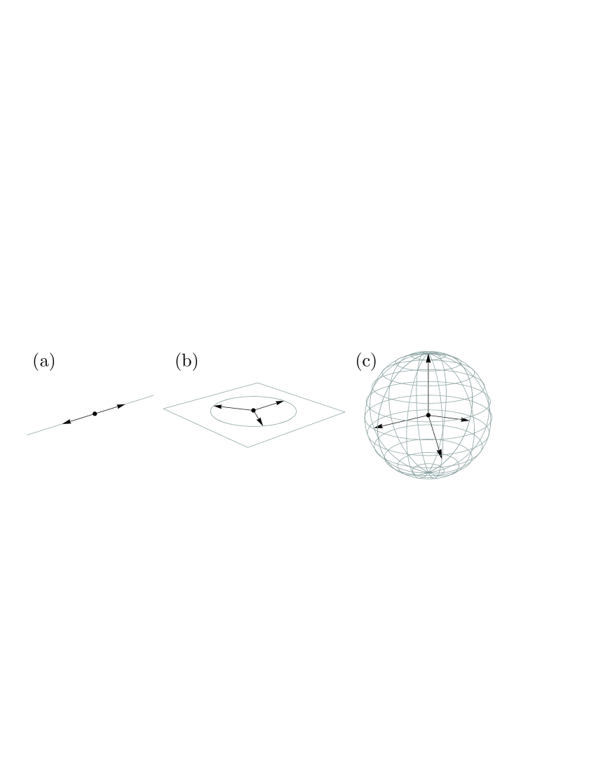
Figure 1: Equiangular vectors in Euclidean spaces: one-dimensional $\mathbb{R}^{1}$ (a), two-dimensional $\mathbb{R}^{2}$ (b), and three-dimensional $\mathbb{R}^{3}$ (c). If the dimension $N$ of space $\mathbb{R}^{N}$ satisfies the condition $N+1=d^{2}$ for some integer $d$, then such equiangular vectors illustrate the SIC projectors $\{\hat{\Pi}_{i}\}_{i=1}^{d^{2}}$ in the Hilbert space $\mathscr{H}_{d}$ ($\mathbb{R}^{d^{2}-1}\sim\mathscr{H}_{d}$).

It is worth mentioning that we have solved incidentally the problem of finding equiangular vectors in Euclidean space $\mathbb{R}^{N}$ (the problem is formulated in wide sense in [66]). Indeed, according to general formula (40), one can introduce the square matrix $\|\mathscr{S}_{N+1}\|$ of any dimension $(N+1)\times(N+1)$ by assuming $N+1=d^{2}$ (here, $d$ is not necessarily an integer). Such a matrix can be rewritten as

$$\|\mathscr{S}_{N+1}\|=\left(\begin{array}[]{ccccc}\displaystyle{\frac{1}{\sqrt[4]{N+1}}}&\displaystyle{\frac{1}{\sqrt[4]{N+1}}}&\displaystyle{\frac{1}{\sqrt[4]{N+1}}}&\cdots&\displaystyle{\frac{1}{\sqrt[4]{N+1}}}\\[8.53581pt] \hline\cr\\[-14.22636pt] {\bf r}_{1}^{(N)}&{\bf r}_{2}^{(N)}&{\bf r}_{3}^{(N)}&\cdots&{\bf r}_{N+1}^{(N)}\\ \end{array}\right),$$ (49)

where we introduced $N$-dimensional vectors ${\bf r}_{i}^{(N)}\in\mathbb{R}^{N}$, $i=1,\ldots,N+1$ such that the scalar product $({\bf r}_{i}^{(N)}\cdot{\bf r}_{j}^{(N)})={\rm const}$ for all $i\neq j$. The explicit form of vectors $\{{\bf r}_{i}^{(N)}\}_{i=1}^{N+1}$ is readily achieved from formula (40) by replacing $d\rightarrow\sqrt{N+1}$. Meanwhile, a similar construction [67] came to our attention. The vectors $\{{\bf r}_{i}^{(N)}\}_{i=1}^{N+1}$ are illustrated in Euclidean spaces $\mathbb{R}^{1}$, $\mathbb{R}^{2}$, and $\mathbb{R}^{3}$ in Fig. 1. The latter case implies $N+1=4=2^{2}$, so it gives a simple illustration of the SIC projectors inside the Bloch ball in $\mathscr{H}_{2}$. Continuing this line of reasoning, we see that SIC projectors can be written in the form $\hat{\Pi}_{i}=\frac{1}{d}\hat{I}_{d\times d}+\left(\hat{\bf E}\cdot{\bf r}_{i}^{(d^{2}-1)}\right)$, where $\hat{\bf E}$ is a vector operator composed of $(d^{2}-1)$ traceless mutually orthogonal operators $\hat{E}_{k}$, ${\rm Tr}\big{[}\hat{E}_{k}^{2}\big{]}=1$, defined through generally unknown orthogonal matrix $\|Q_{\rm SIC}\|$ as follows:

$$\left(\begin{array}[]{c}\frac{1}{\sqrt{d}}\hat{I}\\ \hat{\bf E}\\ \end{array}\right)=\|Q_{\rm SIC}\|^{\rm T}\|\mathfrak{S}\|\hat{\bf D}=\|Q_{\rm SIC}\|^{\rm T}\|\mathfrak{S}^{-1}\|^{\rm T}\hat{\bf S}.$$ (50)

Let us now recall, that unitarily equivalent SIC-POVMs are obtained from each other by applying a unitary transformation $\hat{u}$, i.e., $\hat{\Pi}_{i}\rightarrow\hat{u}\hat{\Pi}_{i}\hat{u}^{{\dagger}}$. In the picture developed, such a transformation results in the transition from one orthogonal basis of operators $\hat{\bf E}$ to the other, i.e., $\hat{E}_{i}\rightarrow\hat{u}\hat{E}_{i}\hat{u}^{{\dagger}}$. As far as orthogonal matrix $\|Q_{\rm SIC}\|$ is concerned, such a transformation is equivalent to multiplication $\|Q_{\rm SIC}\|\rightarrow\|Q_{u}\|\|Q_{\rm SIC}\|$ by an orthogonal matrix $\|Q_{u}\|$ with matrix elements $\|Q_{u}\|_{kl}=\sum_{p,q=1}^{d^{2}}\|\mathfrak{S}^{-1}\|_{pl}\|\mathfrak{S}^{-1}\|_{qk}{\rm Tr}\big{[}\hat{u}\hat{S}_{p}\hat{u}^{{\dagger}}\hat{S}_{q}\big{]}$. Thus, unitary transformation $\hat{u}$ rotates vectors ${\bf r}_{i}^{(d^{2}-1)}$ in the Euclidean space $\mathbb{R}^{d^{2}-1}$ in accordance with the rule ${\bf r}_{i}^{(d^{2}-1)}\rightarrow\sum_{k=1}^{d^{2}}\big{(}\|Q_{\rm SIC}\|^{\rm T}\|Q_{u}\|\|Q_{\rm SIC}\|\big{)}_{ik}{\bf r}_{k}^{(d^{2}-1)}$.

The last remark of this section is that the classification of SIC-POVMs is closely related to the properties of the orthogonal matrix $\|Q_{\rm SIC}\|$.

4 SIC Star-Product Quantization Scheme

In this section, we consider the SIC star-product quantization scheme outlined concisely in Sec. 3.2. The main idea is that, although the exact form of SIC projectors $\hat{\Pi}_{i}$ is not known in general dimension, it is still possible to derive some extra properties of projectors $\hat{\Pi}_{i}$ by assuming that operators

$$\hat{U}_{i}=\frac{1}{d}\hat{\Pi}_{i}{\rm\qquad and\qquad}\hat{D}_{i}=(d+1)\hat{\Pi}_{i}-\hat{I},\qquad i=1,\ldots,d^{2}$$ (51)

are indeed the dequantizer and quantizer, respectively (i.e., define a true quantization scheme). For instance, let us consider properties (12), (2.1) of the star-product kernel $K_{ijk}={\rm Tr}\big{[}\hat{D}_{i}\hat{D}_{j}\hat{U}_{k}\big{]}$ and express them in terms of SIC-projectors’ triple product $T_{ijk}={\rm Tr}\big{[}\hat{\Pi}_{i}\hat{\Pi}_{j}\hat{\Pi}_{k}\big{]}$.

To start, using relation (16) it is not hard to see that the delta-function [in view of formula (8)] on SIC tomographic symbols reads $\mathfrak{D}_{ij}={\rm Tr}\big{[}\hat{U}_{i}\hat{D}_{j}\big{]}=\delta_{ij}$, i.e., reduces to a conventional Kronecker delta-symbol. Further, the star-product kernel reads

$$K_{ijk}=\frac{1}{d}\left[(d+1)^{2}T_{ijk}-d(\delta_{ik}+\delta_{jk})-1\right].$$ (52)

Now, it is possible to calculate the higher-order star-product kernels $K_{ijkl}^{(3)}$ and $K_{ijklm}^{(4)}$ by virtue of several different expressions [see (12), (2.1)]. We omit the intermediate calculations and present, as a result of this consideration, the necessary condition for $T_{ijk}$ to obey

$$\sum_{m=1}^{d^{2}}\left(T_{ijm}T_{mkl}-T_{iml}T_{jkm}\right)=\frac{d}{(d+1)^{3}}\Big{[}(d\delta_{ij}+1)(d\delta_{kl}+1)-(d\delta_{jk}+1)(d\delta_{il}+1)\Big{]},$$ (53)

$$\sum_{n,p=1}^{d^{2}}\left(T_{ijn}T_{nkp}T_{plm}-T_{inp}T_{jkn}T_{plm}\right)=\frac{(d+1)^{2}}{d^{2}}\Bigg{[}\frac{d\delta_{ij}+1}{d+1}T_{klm}+\frac{(d\delta_{ij}+1)(d\delta_{lm}+1)}{(d+1)^{2}}$$

$$\qquad\qquad\qquad\qquad\qquad\qquad\qquad\qquad\qquad\qquad\qquad-T_{ilm}\frac{d\delta_{jk}+1}{d+1}-\frac{(d\delta_{jk}+1)(d\delta_{lm}+1)}{(d+1)^{2}}\Bigg{]},$$ (54)

$$\sum_{n,p=1}^{d^{2}}\left(T_{ijn}T_{nkp}T_{plm}-T_{ijp}T_{kln}T_{pnm}\right)=\frac{(d+1)^{2}}{d^{2}}\Bigg{[}T_{ijk}\frac{d\delta_{lm}+1}{d+1}+\frac{(d\delta_{ij}+1)(d\delta_{lm}+1)}{(d+1)^{2}}$$

$$\qquad\qquad\qquad\qquad\qquad\qquad\qquad\qquad\qquad\qquad\qquad-T_{ijm}\frac{d\delta_{kl}+1}{d+1}-\frac{(d\delta_{ij}+1)(d\delta_{kl}+1)}{(d+1)^{2}}\Bigg{]},\qquad\qquad$$ (55)

where formula (53) corresponds to equality (12), formulas (4) and (4) are responsible for two of five equalities (2.1), with the other being re-expressed through the presented ones. Also, using two expressions for a star-product kernel, namely, the definition (10) and expansions (12) and (2.1), we succeeded in establishing a relation between the triple-product $T_{ijk}$ and the higher-order products, e.g., the four-product ${\rm Tr}\big{[}\hat{\Pi}_{i}\hat{\Pi}_{j}\hat{\Pi}_{k}\hat{\Pi}_{l}\big{]}$ and the five-product ${\rm Tr}\big{[}\hat{\Pi}_{i}\hat{\Pi}_{j}\hat{\Pi}_{k}\hat{\Pi}_{l}\hat{\Pi}_{m}\big{]}$. The result is

$${\rm Tr}\big{[}\hat{\Pi}_{i}\hat{\Pi}_{j}\hat{\Pi}_{k}\hat{\Pi}_{l}\big{]}=\frac{d+1}{d}\sum_{m=1}^{d^{2}}T_{ijm}T_{mkl}-\frac{(d\delta_{ij}+1)(d\delta_{kl}+1)}{(d+1)^{2}},$$ (56)

$${\rm Tr}\big{[}\hat{\Pi}_{i}\hat{\Pi}_{j}\hat{\Pi}_{k}\hat{\Pi}_{l}\hat{\Pi}_{m}\big{]}=\frac{(d+1)^{2}}{d^{2}}\sum_{n,p=1}^{d^{2}}T_{ijn}T_{nkp}T_{plm}$$

$$\qquad\qquad\qquad\qquad\qquad\qquad\qquad-T_{ijk}\frac{d\delta_{lm}+1}{d+1}-\frac{(d\delta_{ij}+1)(d\delta_{lm}+1)}{(d+1)^{2}}-\frac{d\delta_{ij}+1}{d+1}T_{klm}.\qquad\qquad$$ (57)

It is also worth mentioning that the same relations can be obtained (even in an easier way) with the help of the star-product kernel for dual symbols (15) which, in our case, is

$$K_{ijk}^{\rm dual}=\frac{1}{d^{2}(d+1)}\left[(d+1)^{2}T_{ijk}-(d\delta_{ij}+1)\right].$$ (58)

5 SIC-POVMs for Qubits

Let us now develop the above approach to SIC-POVMs for qubits ($d=2$).

To anticipate, the SIC projectors can be chosen as follows:

$$\hat{\Pi}_{1}=\frac{1}{2\sqrt{3}}\left(\begin{array}[]{cc}\sqrt{3}+1&1-i\\ 1+i&\sqrt{3}-1\\ \end{array}\right),\qquad\hat{\Pi}_{2}=\frac{1}{2\sqrt{3}}\left(\begin{array}[]{cc}\sqrt{3}-1&1+i\\ 1-i&\sqrt{3}+1\\ \end{array}\right),$$ (63)

(64)

$$\hat{\Pi}_{3}=\frac{1}{2\sqrt{3}}\left(\begin{array}[]{cc}\sqrt{3}-1&-1-i\\ -1+i&\sqrt{3}+1\\ \end{array}\right),\qquad\hat{\Pi}_{4}=\frac{1}{2\sqrt{3}}\left(\begin{array}[]{cc}\sqrt{3}+1&-1+i\\ -1-i&\sqrt{3}-1\\ \end{array}\right).$$ (69)

It is readily seen that ${\rm Tr}\big{[}\hat{\Pi}_{i}\big{]}={\rm Tr}\big{[}\hat{\Pi}_{i}^{2}\big{]}={\rm Tr}\big{[}\hat{\Pi}_{i}^{3}\big{]}=1$ for all $i=1,\ldots,4$, and ${\rm Tr}\big{[}\hat{\Pi}_{i}\hat{\Pi}_{j}\big{]}=1/3$ if $i\neq j$. The former equality guaranties $\hat{\Pi}_{i}$ to be rank-1 projectors, whereas the latter one shows they are symmetric. The corresponding equiangular vectors in $\mathbb{C}^{2}$ read

$$|\psi_{1}\rangle=\frac{1}{\sqrt{{2\sqrt{3}}}}\left(\begin{array}[]{l}\sqrt{\sqrt{3}+1}\\ \sqrt{\sqrt{3}-1}~{}e^{\mathfrak{i}\pi/4}\\ \end{array}\right),\qquad|\psi_{2}\rangle=\frac{1}{\sqrt{{2\sqrt{3}}}}\left(\begin{array}[]{l}\sqrt{\sqrt{3}-1}\\ \sqrt{\sqrt{3}+1}~{}e^{-\mathfrak{i}\pi/4}\\ \end{array}\right),$$ (74)

(75)

$$|\psi_{3}\rangle=\frac{1}{\sqrt{{2\sqrt{3}}}}\left(\begin{array}[]{l}\sqrt{\sqrt{3}-1}\\ \sqrt{\sqrt{3}+1}~{}e^{\mathfrak{i}3\pi/4}\\ \end{array}\right),\qquad|\psi_{4}\rangle=\frac{1}{\sqrt{{2\sqrt{3}}}}\left(\begin{array}[]{l}\sqrt{\sqrt{3}+1}\\ \sqrt{\sqrt{3}-1}~{}e^{-\mathfrak{i}3\pi/4}\\ \end{array}\right).$$ (80)

5.1 Seeking SIC-POVMs in Dimension $\boldsymbol{d=2}$

To start, we find all possible SIC-POVMs by employing formula (43). The explicit form of the 4$\times$4 matrix $\|\mathscr{S}\|$ reads

$$\|\mathscr{S}\|=\left(\begin{array}[]{cccc}\frac{1}{\sqrt{2}}&\frac{1}{\sqrt{2}}&\frac{1}{\sqrt{2}}&\frac{1}{\sqrt{2}}\\ -\frac{1}{\sqrt{3}}&\frac{1}{\sqrt{3}}&0&0\\ -\frac{1}{3}&-\frac{1}{3}&\frac{2}{3}&0\\ -\frac{1}{3\sqrt{2}}&-\frac{1}{3\sqrt{2}}&-\frac{1}{3\sqrt{2}}&\frac{1}{\sqrt{2}}\\ \end{array}\right).$$ (81)

The $d^{2}$$\times$$d^{2}$ matrix $\|\mathfrak{S}\|$ is given by formulas (37)–(38), which at $d=2$ yield

$$\|\mathfrak{S}\|=\left(\begin{array}[]{cccc}1&0&0&0\\ 0&\cos\theta_{1}&\cos\theta_{2}&\cos\theta_{3}\\ 0&\cos\varphi_{1}\sin\theta_{1}&\cos\varphi_{2}\sin\theta_{2}&\cos\varphi_{3}\sin\theta_{3}\\ 0&\sin\varphi_{1}\sin\theta_{1}&\sin\varphi_{2}\sin\theta_{2}&\sin\varphi_{3}\sin\theta_{3}\\ \end{array}\right)=\left(\begin{array}[]{cccc}1&0&0&0\\ 0&n_{1z}&n_{2z}&n_{3z}\\ 0&n_{1x}&n_{2x}&n_{3x}\\ 0&n_{1y}&n_{2y}&n_{3y}\\ \end{array}\right),\qquad\quad$$ (82)

whereas, according to formula (4), the vector operator $\hat{\bf S}$ reads

$$\hat{\bf S}\equiv\left(\begin{array}[]{c}\hat{S}_{0}^{(1/2)}({\bf n}_{1})\\ \hat{S}_{1}^{(1/2)}({\bf n}_{1})\\ \hat{S}_{1}^{(1/2)}({\bf n}_{2})\\ \hat{S}_{1}^{(1/2)}({\bf n}_{3})\\ \end{array}\right)=\left(\begin{array}[]{c}\frac{1}{\sqrt{2}}\hat{I}\\ \sqrt{2}(\hat{\bf J}\cdot{\bf n}_{1})\\ \sqrt{2}(\hat{\bf J}\cdot{\bf n}_{2})\\ \sqrt{2}(\hat{\bf J}\cdot{\bf n}_{3})\\ \end{array}\right)=\frac{1}{\sqrt{2}}\left(\begin{array}[]{c}\hat{I}\\ (\hat{\boldsymbol{\sigma}}\cdot{\bf n}_{1})\\ (\hat{\boldsymbol{\sigma}}\cdot{\bf n}_{2})\\ (\hat{\boldsymbol{\sigma}}\cdot{\bf n}_{3})\\ \end{array}\right).$$ (83)

Substituting (81) for $\|\mathscr{S}\|$, (82) for $\|\mathfrak{S}\|$, and (83) for $\hat{\bf S}$ in (43), after simplification, we obtain

$$\hat{\boldsymbol{\Pi}}=\frac{1}{2}\left(\begin{array}[]{cccc}1&-\sqrt{\frac{2}{3}}&-\frac{\sqrt{2}}{3}&-\frac{1}{3}\\ 1&\sqrt{\frac{2}{3}}&-\frac{\sqrt{2}}{3}&-\frac{1}{3}\\ 1&0&\frac{2\sqrt{2}}{3}&-\frac{1}{3}\\ 1&0&0&1\\ \end{array}\right)\left(\begin{array}[]{c|ccc}1&0&0&0\\ \hline\cr 0&\lx@intercol\hfil\hfil\lx@intercol\\ 0&\lx@intercol\hfil\widetilde{Q}^{\rm T}\hfil\lx@intercol\\ 0&\lx@intercol\hfil\hfil\lx@intercol\\ \end{array}\right)\left(\begin{array}[]{c}\hat{I}\\ \hat{\sigma}_{z}\\ \hat{\sigma}_{x}\\ \hat{\sigma}_{y}\\ \end{array}\right)=\frac{1}{2}\left(\begin{array}[]{c}\hat{I}+(\hat{\boldsymbol{\sigma}}\cdot\|R\|{\bf r}_{1})\\ \hat{I}+(\hat{\boldsymbol{\sigma}}\cdot\|R\|{\bf r}_{2})\\ \hat{I}+(\hat{\boldsymbol{\sigma}}\cdot\|R\|{\bf r}_{3})\\ \hat{I}+(\hat{\boldsymbol{\sigma}}\cdot\|R\|{\bf r}_{4})\\ \end{array}\right),\qquad$$ (84)

where we introduce a 3$\times$3 orthogonal matrix $\|R\|$ and normalized vectors $\{{\bf r}_{i}\}_{i=1}^{4}\in\mathbb{R}^{3}$ given by

$$\|R\|=\left(\begin{array}[]{ccc}0&1&0\\ 0&0&1\\ 1&0&0\\ \end{array}\right)\|\widetilde{Q}\|,~{}{\bf r}_{1}=\left(\begin{array}[]{c}-\sqrt{\frac{2}{3}}\\ -\frac{\sqrt{2}}{3}\\ -\frac{1}{3}\\ \end{array}\right),~{}{\bf r}_{2}=\left(\begin{array}[]{c}\sqrt{\frac{2}{3}}\\ -\frac{\sqrt{2}}{3}\\ -\frac{1}{3}\\ \end{array}\right),~{}{\bf r}_{3}=\left(\begin{array}[]{c}0\\ \frac{2\sqrt{2}}{3}\\ -\frac{1}{3}\\ \end{array}\right),~{}{\bf r}_{4}=\left(\begin{array}[]{c}0\\ 0\\ 1\\ \end{array}\right).\quad$$ (85)

It is shown in Sec. 3.4 that, if the set of operators $\{\hat{\Pi}_{i}\}_{i=1}^{4}$ is constructed in such a way, then the hermicity condition (26) as well as the trace conditions (27) and (28) of the first and second orders, respectively, is fulfilled automatically. For $\{\hat{\Pi}_{i}\}_{i=1}^{4}$ to be true SIC projectors, the extra restriction on orthogonal matrix $\|Q\|$ is imposed by requirement (47) or an equivalent requirement (48). In our case, these restrictions can be easily written in terms of the 3$\times$3 matrix $\|R\|$. Surprisingly enough that, in the case of qubits, these additional conditions are also fulfilled for an arbitrary orthogonal matrix $\|R\|$. This means that formula (84) gives the explicit solution to the problem of SIC existence, with one SIC-POVM construction differing from the other in the choice of the orthogonal matrix $\|R\|$ only. The geometrical sense of this fact in the Bloch ball picture in Fig. 1c is that all possible sets of SIC projectors $\{\hat{\Pi}_{i}\}_{i=1}^{4}$ (unambiguously defined by vectors $\{{\bf r}_{i}\}_{i=1}^{4}$) are obtained by applying an orthogonal transformation to all the vectors $\{{\bf r}_{i}\}_{i=1}^{4}$ simultaneously. For example, the SIC projectors (63) are obtained from formula (84) by an orthogonal transformation $\|R\|$ which transforms vectors (85) into vectors $\frac{1}{\sqrt{3}}(1,1,1)$, $\frac{1}{\sqrt{3}}(1,-1,-1)$, $\frac{1}{\sqrt{3}}(-1,1,-1)$, and $\frac{1}{\sqrt{3}}(-1,-1,1)$. Among all possible orthogonal transformations $\|R\|$, one can point out the case of rotation ($\det\|R\|=1$) and inversion ($\det\|R\|=-1$). Therefore, we have two SIC-POVM sets generated by fixed representation operator, namely, the Weyl–Heisenberg displacement operator. To be concise, we have two different fiducial vectors, such that one vector can be obtained from the other by inversion of the Bloch ball picture [50].

5.2 Star-Product Kernel for Qubits

Now, when the SIC projectors are found, let us explore their properties.

To start, we focus our attention on the star-product kernel $K_{ijk}$ which is connected with many additional relations, e.g., (53)–(57). Employing well-known properties of Pauli matrices, it is not hard to see that the triple-product $T_{ijk}={\rm Tr}\big{[}\hat{\Pi}_{i}\hat{\Pi}_{j}\hat{\Pi}_{k}\big{]}$ reads

$$T_{ijk}=\frac{1}{4}\Big{\{}1+({\bf r}_{i}\cdot{\bf r}_{j})+({\bf r}_{j}\cdot{\bf r}_{k})+({\bf r}_{k}\cdot{\bf r}_{i})+\mathfrak{i}({\bf r}_{i}\cdot[{\bf r}_{j}\times{\bf r}_{k}])\Big{\}},$$ (86)

where $\mathfrak{i}$ is the imaginary unit and $({\bf r}_{i}\cdot[{\bf r}_{j}\times{\bf r}_{k}])$ denotes the standard triple product of vectors. Further, we take into account that, in our case, $({\bf r}_{i}\cdot{\bf r}_{j})=(4\delta_{ij}-1)/3$ and $({\bf r}_{i}\cdot[{\bf r}_{j}\times{\bf r}_{k}])=-4\varepsilon_{ijk}/3\sqrt{3}$, where $\varepsilon_{ijk}$ is an antisymmetric tensor such that $\varepsilon_{123}=\varepsilon_{134}=\varepsilon_{142}=\varepsilon_{432}=1$. Finally, using (52) and (58), we obtain

$$T_{ijk}=\frac{1}{3}\Big{\{}\delta_{ij}+\delta_{jk}+\delta_{ki}-\frac{\mathfrak{i}}{\sqrt{3}}\varepsilon_{ijk}\Big{\}},\qquad K_{ijk}=\frac{1}{2}\Big{\{}3\delta_{ij}-\mathfrak{i}\sqrt{3}\varepsilon_{ijk}-1\Big{\}},$$ (87)

$$K_{ijk}^{\rm dual}=\frac{1}{12}\Big{\{}\delta_{ij}+3(\delta_{jk}+\delta_{ki})-\mathfrak{i}\sqrt{3}\varepsilon_{ijk}-1\Big{\}}.$$ (88)

It is known that there exists a recurrence relation on star-product kernels of spin-tomographic symbols $w(m,{\bf n})$ (see the family of spin-tomographic symbols in Sec. 2) which connects the kernel of spin $j$ with the kernels of spins $(j-1/2)$ and $(j-1)$ [68]. We hope that a similar relation does exist for SIC tomographic kernels $K_{ijk}$ as well. In this case, such a relation would connect kernels for dimensions $d$, $(d-1)$, and $(d-2)$.

5.3 Intertwining Kernels to Other Quantization Schemes

We emphasize here that the SIC representation of quantum states (Sec. 3.1) is closely related to other probability representations of quantum mechanics. This means that there exists a relation between the SIC quantization scheme and other quantization schemes. This section is devoted to establishing such a relation between SIC tomographic symbols $f_{A}(i)\equiv{\rm Tr}\big{[}\hat{A}\hat{U}_{i}\big{]}$ and spin-tomographic symbols $f_{A}(m,{\bf n})$ as well as spin-FNR tomographic symbols $f_{A}(m,{\bf n}_{k})$ (spin tomography with a finite number of rotations) outlined briefly in Sec. 2.

In fact, utilizing general relations (1) and (2) of the star product, we immediately obtain the following relation between two quantization schemes ${\bf x}_{1}$ and ${\bf x}_{2}$:

$$f_{A}({\bf x}_{2})=\int f_{A}({\bf x}_{1}){\rm Tr}\big{[}\hat{D}({\bf x}_{1})\hat{U}({\bf x}_{2})\big{]}d{\bf x_{1}}.$$ (89)

We will refer to the kernel $\mathcal{K}_{1\rightarrow 2}({\bf x}_{1},{\bf x}_{2}):={\rm Tr}\big{[}\hat{D}({\bf x}_{1})\hat{U}({\bf x}_{2})\big{]}$ as the intertwining kernel between schemes ${\bf x}_{1}$ and ${\bf x}_{2}$. Applying formula (89) to qubits, we readily obtain the explicit form of the intertwining kernels between the SIC quantization scheme [determined by SIC projectors (84)] and alternative quantization schemes given by (3), (5), (6), and vice versa. The result is

$$\mathcal{K}_{\rm Spin\rightarrow SIC}(m,{\bf n},i)=\frac{1}{4}\Big{(}1+6m({\bf n}\cdot\|R\|{\bf r}_{i})\Big{)},$$ (90)

$$\mathcal{K}_{\rm SIC\rightarrow Spin}(i,m,{\bf n})=\frac{1}{2}\Big{(}1+6m({\bf n}\cdot\|R\|{\bf r}_{i})\Big{)},$$ (91)

$$\mathcal{K}_{\rm SpinFNR\rightarrow SIC}(m,{\bf n}_{k},i)=\frac{3}{4}\Big{(}\delta_{k,1}+2m({\bf l}_{k}\cdot\|R\|{\bf r}_{i})\Big{)},$$ (92)

$$\mathcal{K}_{\rm SIC\rightarrow SpinFNR}(i,m,{\bf n}_{k})=\frac{1}{6}\Big{(}1+6m({\bf n}_{k}\cdot\|R\|{\bf r}_{i})\Big{)},$$ (93)

with vectors ${\bf l}_{k}$, $k=1,2,3$ in Eq. (92) forming a dual basis with respect to the directions $\{{\bf n}_{k}\}_{k=1}^{3}$ [25].

5.4 Relation to Mutually Unbiased Bases

It is known that the SIC construction and so-called mutually unbiased bases (MUBs) have some common properties [69, 70]. In order to illustrate this relation, we restrict ourselves to the case of qubits only. Using the standard notation $|\uparrow\rangle:=|j=1/2,m=1/2\rangle$, $|\downarrow\rangle:=|j=1/2,m=-1/2\rangle$, one can introduce three bases $\big{\{}|\mu_{i}\rangle,|\nu_{i}\rangle\big{\}}_{i=1}^{3}$ such that $\langle\mu_{i}|\nu_{i}\rangle=0$ for all $i=1,2,3$ and $\left|\langle\mu_{i}|\mu_{j}\rangle\right|^{2}=\left|\langle\mu_{i}|\nu_{j}\rangle\right|^{2}=\left|\langle\nu_{i}|\nu_{j}\rangle\right|^{2}=1/2$ for all $i\neq j$. Indeed, a possible choice of MUBs is as follows:

$$|\mu_{1}\rangle=|\uparrow\rangle,\quad|\nu_{1}\rangle=|\downarrow\rangle,\qquad|\mu_{2}\rangle=\frac{|\uparrow\rangle+|\downarrow\rangle}{\sqrt{2}},\quad|\nu_{2}\rangle=\frac{|\uparrow\rangle-|\downarrow\rangle}{\sqrt{2}},$$

(94)

$$|\mu_{3}\rangle=\frac{|\uparrow\rangle+\mathfrak{i}|\downarrow\rangle}{\sqrt{2}},\quad|\nu_{3}\rangle=\frac{|\uparrow\rangle-\mathfrak{i}|\downarrow\rangle}{\sqrt{2}}.$$

The states (5.4) correspond to the following points on the Bloch sphere: $(0,0,1)$, $(0,0,-1)$, $(1,0,0)$, $(-1,0,0)$, $(0,1,0)$, and $(0,-1,0)$, respectively (see Fig. 1c). These points are nothing else but vertices of the octahedron. Each basis $\big{\{}|\mu_{i}\rangle,|\nu_{i}\rangle\big{\}}$ corresponds to the $i$th diagonal of the octahedron. In view of this, similar to SIC-POVMs which are associated with diagonals of the cube, the MUBs are also associated with equiangular lines, namely, diagonals of the octahedron. It is worth mentioning that the problem of existence of MUBs in $\mathscr{H}_{d}$ of any dimension $d$ can also be formulated in terms of symbols of operators.

6 Notes to Lie Algebraic Consideration

It is emphasized in [51] that the $d^{2}$ operators $\{\hat{\Pi}_{i}\}_{i=1}^{d^{2}}$ form a basis for the complex Lie algebra ${\rm gl}(d,\mathbb{C})$ and satisfy the commutation relation of the form

$$\big{[}\hat{\Pi}_{i},\hat{\Pi}_{j}\big{]}=\sum_{k=1}^{d^{2}}J_{ijk}\hat{\Pi}_{k}.$$ (95)

Structure constants $J_{ijk}$ are expressed through the kernel $K_{ijk}$ as follows:

$$J_{ijk}=\frac{1}{d+1}\left(K_{ijk}-K_{jik}\right).$$ (96)

Formula (96) is a standard relation between the structure constants of associative product and the structure constants of the Lie product. In order to derive new relations on projectors $\hat{\Pi}_{i}$ originating from their Lie algebraic structure, we will consider case $d=2$ in detail. In this case, we have connection with the Lie group ${\rm GL}(2,\mathbb{C})$. This group can be considered as a direct product of the group ${\rm SL}(2,\mathbb{C})$ and the group of complex numbers with the standard multiplication rule. The matrices that belong to the group ${\rm SL}(2,\mathbb{C})$ are the matrices of the Lorentz-group representation. Generators $H_{1}$, $H_{2}$, $H_{3}$, $F_{1}$, $F_{2}$, and $F_{3}$ of ${\rm SL}(2,\mathbb{C})$ read [71]

$$H_{1}=\mathfrak{i}F_{1}=\frac{1}{2}\left(\begin{array}[]{cc}0&1\\ 1&0\\ \end{array}\right),\quad H_{2}=\mathfrak{i}F_{2}=\frac{1}{2}\left(\begin{array}[]{cc}0&\mathfrak{i}\\ -\mathfrak{i}&0\\ \end{array}\right),\quad H_{3}=\mathfrak{i}F_{3}=\frac{1}{2}\left(\begin{array}[]{cc}1&0\\ 0&-1\\ \end{array}\right)$$ (97)

and satisfy commutation relations of the form

$$\big{[}H_{\pm},H_{3}\big{]}=\mp H_{\pm},\quad\big{[}H_{+},H_{-}\big{]}=2H_{3},\quad\big{[}F_{\pm},F_{3}\big{]}=\pm H_{\pm},\quad\big{[}F_{+},F_{-}\big{]}=-2H_{3},$$

(98)

$$\big{[}F_{+},H_{+}\big{]}=\big{[}H_{-},F_{-}\big{]}=\big{[}H_{3},F_{3}\big{]}=0,\quad\big{[}H_{\pm},F_{\mp}\big{]}=\pm 2F_{3},\quad\big{[}F_{\pm},H_{3}\big{]}=\mp F_{\pm},$$

where $H_{\pm}=H_{1}\pm\mathfrak{i}H_{2}$, $F_{\pm}=F_{1}\pm\mathfrak{i}F_{2}$, and $\mathfrak{i}$ is the imaginary unit. Further, there exist two Casimir operators $\hat{C}_{1}$ and $\hat{C}_{2}$ (see the explicit form, e.g., in [72])

$$\hat{C}_{1}=\hat{\bf H}^{2}-\hat{\bf F}^{2}+2\mathfrak{i}(\hat{\bf H}\cdot\hat{\bf F}),\qquad\hat{C}_{2}=\hat{\bf H}^{2}-\hat{\bf F}^{2}-2\mathfrak{i}(\hat{\bf H}\cdot\hat{\bf F}),$$ (99)

such that $\big{[}\hat{C}_{1},\hat{H}_{i}\big{]}=\big{[}\hat{C}_{1},\hat{F}_{i}\big{]}=\big{[}\hat{C}_{2},\hat{H}_{i}\big{]}=\big{[}\hat{C}_{2},\hat{F}_{i}\big{]}=0$ for all $i=1,2,3$. It is worth mentioning that operators $\frac{1}{2}(\hat{C}_{1}+\hat{C}_{2})$ and $\frac{1}{2\mathfrak{i}}(\hat{C}_{1}-\hat{C}_{2})$ have the sense of Lorentz invariants of the electromagnetic field.

Let us rewrite these commutation relations in terms of projectors $\hat{\Pi}_{i}$, assuming that only the commutation relation (95) is known. Indeed, we will then obtain a new restriction onto projectors $\hat{\Pi}_{i}$ originating from their Lie algebraic structure.

In the case $d=2$, relation (95) transforms into $\big{[}\hat{\Pi}_{i},\hat{\Pi}_{j}\big{]}=\pm\sum_{k=1}^{4}\frac{\mathfrak{i}}{\sqrt{3}}\varepsilon_{ijk}\hat{\Pi}_{k}$, where $\varepsilon_{ijk}$ is an antisymmetric tensor such that $\varepsilon_{123}=\varepsilon_{134}=\varepsilon_{142}=\varepsilon_{432}=1$ and the sign $\pm$ depends on the labeling of the SIC projectors (we choose the plus sign). Suppose now

$$\hat{H}_{1}=\mathfrak{i}\hat{F}_{1}=\frac{\sqrt{3}}{8}\left(\hat{\Pi}_{1}+\hat{\Pi}_{2}-\hat{\Pi}_{3}-\hat{\Pi}_{4}\right),$$

$$\hat{H}_{2}=\mathfrak{i}\hat{F}_{2}=\frac{\sqrt{3}}{8}\left(-\hat{\Pi}_{1}+\hat{\Pi}_{2}-\hat{\Pi}_{3}+\hat{\Pi}_{4}\right),$$ (100)

$$\hat{H}_{3}=\mathfrak{i}\hat{F}_{3}=\frac{\sqrt{3}}{8}\left(\hat{\Pi}_{1}-\hat{\Pi}_{2}-\hat{\Pi}_{3}+\hat{\Pi}_{4}\right),$$

then Casimir operators (99) take the form

$$\hat{C}_{1}=0,\qquad\hat{C}_{2}=\frac{3}{16}\left(3\sum_{i=1}^{4}\hat{\Pi}_{i}^{2}-\sum_{i\neq j}\hat{\Pi}_{i}\hat{\Pi}_{j}\right).$$ (101)

Finally, starting from commutators (95) and using a specific property of Casimir operators, we manage to obtain the following commutation relations:

$$\left[\hat{\Pi}_{k},3\sum_{i=1}^{4}\hat{\Pi}_{i}^{2}-\sum_{i\neq j}\hat{\Pi}_{i}\hat{\Pi}_{j}\right]=0{\rm~{}for~{}all~{}}k=1,\ldots,4.$$ (102)

In fact, relations similar to (102) can also be derived in higher dimensions. The crucial point is that the obtained equation is compatible with conditions (20)–(24). Thus, if SIC-POVMs do exist, the whole series of operator conditions (20)–(24)$\wedge$(102, generalized) is to be fulfilled simultaneously.

7 Conclusions

To conclude, we present the main results of the paper.

Combining the ideas of a generic star-product scheme with the SIC-POVM approach to quantum states, we have shown that the SIC projectors $\hat{\Pi}_{i}$ can be considered (up to a normalization factor and the identity operator) as dequantizers $\hat{U}_{i}$ and quantizers $\hat{D}_{i}$ of the SIC star-product quantization scheme. From this, it follows immediately that fulfilling of conditions (20)–(24) means the existence of the associative product $K_{ijk}={\rm Tr}\big{[}\hat{D}_{i}\hat{D}_{j}\hat{U}_{k}\big{]}$ which is a solution of Eqs. (12) and (2.1). Moreover, utilizing the standard equations for a generic star-product kernel, we have derived some properties of the triple products $T_{ijk}={\rm Tr}\big{[}\hat{\Pi}_{i}\hat{\Pi}_{j}\hat{\Pi}_{k}\big{]}$ of SIC projectors found in [51]. Thus, we have interpreted such properties of $T_{ijk}$ as standard properties of the star-product kernel (including the dual [55] star-product scheme). From the same point of view, the Lie algebraic structure found in [51] is an immediate and known consequence of the antisymmetrized kernel of associative product. Further, the problem of SIC-POVM existence is formulated in terms of symbols of the SIC projectors and the corresponding kernel of associative product (26)–(29). The approach to solve the modified problem is also developed. By example of qubits, we show the similarity between SIC-POVMs and mutually unbiased bases (MUBs) and hope to clarify this connection elsewhere.

The other result of this work is the conclusion that the SIC-POVM is a partial case of the probability representation of quantum states and can be related to other known kinds of the probability representations like the spin tomography, unitary tomography, and spin tomography with a finite number of rotations. Also, we cannot help mentioning a conceptual drawback of the SIC representation, namely, the absence of a measurable physical quantity which can give rise to the SIC probability distribution.

References

- [1] M. A. Man’ko, J. Russ. Laser Res., 21, 411 (2000).
- [2] M. A. Man’ko, J. Russ. Laser Res., 22, 48 (2001).
- [3] M. A. Man’ko, J. Russ. Laser Res., 23, 433 (2002).
- [4] M. A. Man ko, J. Russ. Laser Res., 27, 405 (2006).
- [5] M. A. Man’ko, J. Russ. Laser Res., 22, 168 (2001).
- [6] R. Fedele and M. A. Man’ko, Eur. Phys. J. D, 27, 263 (2003).
- [7] M. A. Man’ko, O. V. Man’ko, and V. I. Man’ko, Int. J. Mod. Phys. D, 20, 1399 (2006).
- [8] M. A. Man’ko, J. Russ. Laser Res., 27, 507 (2006).
- [9] M. A. Man ko, J. Russ. Laser Res., 30, 514 (2009).
- [10] M. A. Man’ko and V. I. Man’ko, Found. Phys., DOI 10.1007/s10701-009-9403-9 (2009).
- [11] S. Mancini, V. I. Man’ko, and P. Tombesi, Phys. Lett. A, 213, 1 (1996).
- [12] S. Mancini, V. I. Man’ko, and P. Tombesi, Found. Phys., 27, 801 (1997).
- [13] E. Schrödinger, Ann. Phys., Lpz., 79, 489 (1926).
- [14] L. D. Landau, Ztschr. Physik, 45, 430 (1927).
- [15] J. von Neumann, Göttingen. Nachr., 245 (1927).
- [16] E. P. Wigner, Phys. Rev., 40, 749 (1932).
- [17] K. Husimi, Proc. Phys. Math. Soc. Jpn, 22, 264 (1940).
- [18] E. C. G. Sudarshan, Phys. Rev. Lett., 10, 177 (1963).
- [19] R. J. Glauber, Phys. Rev. Lett., 10, 84 (1963).
- [20] J. Radon, Ber. Verh. Saechs. Akad. Wiss. Leipzig, Math.-Phys. Kl., 69, 262 (1917).
- [21] I. M. Gel’fand and G. E. Shilov, Generalized Functions: Properties and Operations, Academic Press, New York (1966), Vol. 5.
- [22] V. V. Dodonov and V. I. Man’ko, Phys. Lett. A, 229, 335 (1997).
- [23] V. I. Man’ko and O. V. Man’ko, J. Exp. Theor. Phys., 85, 430 (1997).
- [24] S. N. Filippov and V. I. Man’ko, J. Russ. Laser Res., 30, 129 (2009).
- [25] S. N. Filippov and V. I. Man’ko, J. Russ. Laser Res., 31, 32 (2010).
- [26] S. N. Filippov and V. I. Man’ko, “Distances between quantum states in the tomographic-probability representation,” arXiv:0911.1414v1 [quant-ph] (2009).
- [27] A. Ibort, V. I. Man’ko, G. Marmo, et al., Phys. Scr., 79, 065013 (2009).
- [28] J. Bertrand and P. Bertrand, Found. Phys., 17, 397 (1987).
- [29] K. Vogel and H. Risken, Phys. Rev. A, 40, 2847 (1989).
- [30] S. Mancini, V. I. Man’ko, and P. Tombesi, Quantum Semiclass. Opt., 7, 615 (1995).
- [31] K. Banaszek and K. Wodkiewicz, Phys. Rev. Lett., 76, 4344 (1996).
- [32] S. Wallentowitz and W. Vogel, Phys. Rev. A, 53, 4528 (1996).
- [33] S. Mancini, P. Tombesi, and V. I. Man’ko, Europhys. Lett., 37, 79 (1997).
- [34] M. Asorey, P. Facchi, V. I. Man’ko, et al., Phys. Rev. A, 77, 042115 (2008).
- [35] M. Asorey, P. Facchi, G. Florio, et al, “Robustness of raw quantum tomography,” arXiv:1003.1664v1 [quant-ph] (2010).
- [36] S. T. Ali and E. Prugovečki, J. Math. Phys., 18, 219 (1977).
- [37] S. T. Ali and E. Prugovečki, Physica A, 89, 501 (1977).
- [38] S. T. Ali and E. Prugovečki, Int. J. Theor. Phys., 16, 689 (1977).
- [39] P. Busch and P. J. Lahti, Found. Phys., 19, 633 (1989).
- [40] P. Busch, G. Cassinelli, and P. J. Lahti, Rev. Math. Phys., 7, 1105 (1995).
- [41] P. Busch, M. Grabowski, and P. J. Lahti, Operational Quantum Physics, Lecture Notes in Physics, Springer-Verlag, Berlin (1995), Vol. 31.
- [42] W. Stulpe, Found. Phys., 24, 1089 (1994).
- [43] W. Stulpe, Int. J. Theor. Phys., 37, 349 (1998).
- [44] W. Stulpe, “Classical representations of quantum mechanics related to statistically complete observables,” Los Alamos Arxiv, quant-ph/0610122 (2006).
- [45] J. Kiukas, P. Lahti, and J.-P. Pellonpää, J. Phys. A: Math. Theor., 41, 175206 (2008).
- [46] J.-P. Amiet and S. Weigert, J. Phys. A: Math. Gen., 32, L269 (1999).
- [47] R. G. Newton and B. Young, Ann. Phys., 49, 393 (1968).
- [48] C. M. Caves, “Symmetric informationally complete POVMs,” UNM Information Physics Group internal report, http://info.phys.unm.edu/ caves/reports/infopovm.pdf (1999).
- [49] C. M. Caves, C. A. Fuchs, and R. Schack, Phys. Rev. A, 65, 022305 (2002).
- [50] J. M. Renes, R. Blume-Kohout, A. J. Scott, and C. M. Caves, J. Math. Phys., 45, 2171 (2004).
- [51] D. M. Appleby, S. T. Flammia, and C. A. Fuchs, “The Lie algebraic significance of symmetric informationally complete measurements,” arXiv:1001.0004v1 [quant-ph] (2010).
- [52] C. A. Fuchs, “Quantum Bayesianism at the Perimeter,” arXiv:1003.5182v1 [quant-ph] (2010).
- [53] R. L. Stratonovich, Sov. Phys. JETP, 4, 891 (1957).
- [54] O. V. Man’ko, V. I. Man’ko, and G. Marmo, J. Phys. A: Math. Gen., 35, 699 (2002).
- [55] O. V. Man’ko, V. I. Man’ko, G. Marmo, and P. Vitale, Phys. Lett. A, 360, 522 (2007).
- [56] S. N. Filippov and V. I. Man’ko, J. Russ. Laser Res., 30, 224 (2009).
- [57] S. N. Filippov and V. I. Man’ko, Phys. Scr., 79, 055007 (2009).
- [58] A. F. Nikiforov, S. K. Suslov, and V. B. Uvarov, Classical Orthogonal Polynomials of a Discrete Variable, Springer-Verlag, Berlin, Heidelberg, New York (1991).
- [59] V. I. Man’ko, G. Marmo, E. C. G. Sudarshan, and F. Zaccaria, Phys. Lett. A, 327, 353 (2004).
- [60] A. J. Scott and M. Grassl, J. Math. Phys., 51, 042203 (2010).
- [61] D. M. Appleby, Å. Ericsson and C. A. Fuchs, Found. Phys., DOI: 10.1007/s10701-010-9458-7 (2010).
- [62] S. Weigert, Phys. Rev. Lett., 84, 802 (2000).
- [63] V. I. Man’ko, G. Marmo, A. Simoni, et al., Rep. Math. Phys., 61, 337 (2008).
- [64] N. S. Jones and N. Linden, Phys. Rev. A, 71, 012324 (2005).
- [65] F. R. Gantmacher, The Theory of Matrices, AMS Chelsea Publishing, Providence, RI (1998).
- [66] P. W. H. Lemmens and J. J. Seidel, J. Algebra, 24, 494 (1973).
- [67] J. C. Tremain, “Concrete constructions of real equiangular line sets,” arXiv:0811.2779v1 [math.MG] (2008).
- [68] S. N. Filippov and V. I. Man’ko, J. Russ. Laser Res., 30, 224 (2009).
- [69] O. Albouy and M. R. Kibler, J. Russ. Laser Res., 28, 429 (2007).
- [70] D. M. Appleby, “SIC-POVMs and MUBs: geometrical relationships in prime dimension,” arXiv:0905.1428v1 [quant-ph] (2009).
- [71] I. M. Gel’fand, R. A. Minlos, and Z. Ya. Shapiro, Representations of the Rotation and Lorentz Groups and Their Applications, The Macmillan Company, New York (1963).
- [72] Ya. A. Smorodinskii and M. Huszar, Theor. Math. Phys., 4, 867 (1970).