Abstract

A small and light polystyrene ball is released without initial speed from a certain height above the floor. Then, it falls on air. The main responsible for the friction force against the movement is the wake of successive air vortices which form behind (above) the falling ball, a turbulent phenomenon. After the wake appears, the friction force compensates the Earth gravitational attraction and the ball speed stabilises in a certain limiting value $V_{\ell}$. Before the formation of the turbulent wake, however, the friction force is not strong enough, allowing the initially growing speed to surpass the future final value $V_{\ell}$. Only after the wake finally becomes long enough, the ball speed decreases and reaches the proper $V_{\ell}$.

1 Introduction

While teaching Physics at their universities for undergraduate students, the authors designed a simple didactic experiment in order to exhibit the influence of air flow around falling objects. An unexpected behaviour was found, its explanation being beyond undergraduate Physics. Previously, a simple, home-made version of the experiment presented here was performed, using a staircase, a tape measure and a hand chronometer, as follows. A polystyrene ball with diameter $D\approx 2.5{\rm cm}$ and mass $m\approx 0.2{\rm g}$ is released from a height $X$ above the floor, and the falling time $T$ is measured.

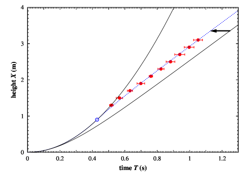
Figure 1: Falling time for different heights. The vertical error bars are negligible. The horizontal error bar displayed for each experimental point (red) is calculated from the statistics of 10 repeated time measurements. Using the Earth gravitational field $g=9.8{\rm m/s^{2}}$, the upper curve is the free fall parabola, $X=g\,T^{2}/2$, no friction at all. The other two curves correspond to an air friction force proportional to the squared speed. At the lower curve, this force acts during the whole fall, since beginning. At the intermediate, dotted curve (blue), the same friction force is turned on only after an adjusted initial transient time (open blue bullet), with no friction before that. Note that the slope of this curve has a maximum around $\approx 0.4{\rm s}$. Note also that the observed fall is in advance by more than $0.1{\rm s}$ (arrow), relative to the lower curve.

The procedure is repeated 10 times for each height, in order to determine the experimental uncertainty and the consequent error bars. The result is displayed by the bullets with horizontal error bars in figure 1.

The traditional free fall model, $X=g\,T^{2}/2$, obviously does not fit the experimental data, perhaps with the exception of the two first experimental points obtained for the smallest measured heights. Therefore, somehow the influence of the air flow around the ball should be taken into account. The two first experimental points positioned near the parabola indicate a deviation from the free fall only after a certain transient time, during which the influence of the air around the falling ball seems negligible.

Ruled out the free fall, the next simplest model one can try is the also traditional Stokes friction force, $F=3\pi D\eta V$ for a ball running with constant speed $V$ on a viscous fluid with viscosity $\eta$. This formula is valid only while the air flow around the ball is laminar, without turbulent vortices, which does not correspond to our experimental conditions. Even so, we can estimate the order of magnitude $F\approx 10^{-5}{\rm N}$ of this force by taking the maximum observed speed $V\approx 4{\rm m/s}$, and by using the air viscosity $\eta\approx 2\times 10^{-5}{\rm kg/m.s}$. It is therefore negligible, two orders of magnitude smaller than the ball weight $mg\approx 2\times 10^{-3}{\rm N}$. So, we can conclude that it is not the Stokes laminar flow friction proportional to $V$ which matters within our experiment.

Indeed, a Reynolds number ${\cal R}\approx 6\times 10^{3}$ can be estimated for $V\approx 4{\rm m/s}$. (The Reynolds number defined as ${\cal R}=\rho\,V\,D/\eta$, where $\rho\approx 1.2{\rm kg/m^{3}}$ is the air density, is the main index to evaluate the various possible regimes of the air flow around the ball, laminar, turbulent, etc.) For $10^{3}<{\cal R}<10^{5}$, the friction force is experimentally known to be proportional to the squared speed within a good accuracy, and also much larger than the Stokes laminar prediction. The experiments are performed in wind tunnels, with the ball fixed under a constant wind speed, which again are not the same conditions of our experiment.

Besides measuring the friction force, these wind tunnel experiments also allow to measure the air velocities in different points near the ball at different times. The outcome is the so-called von Kármán vortex street, a wake of successive air vortices which form behind the ball, extending for distances corresponding to hundred diameters downstream. The turbulent vortex dynamics is the following. One vortex forms near the ball and slowly goes away. When its distance from the ball reaches some few diameters, a second vortex forms near the ball, which also slowly goes away. Then, a third vortex forms again near the ball, and so on. After some time, there is a complete wake of many successive vortices behind the ball, the street.

By following the movement of one particular vortex, one notes that its speed is much smaller than the wind speed itself (far from the ball and the wake). Therefore, somehow the ball drags the vortex wake behind it. According to the third Newton’s law, the reaction force exerted by the wake on the ball substantially enhances the friction force against the movement, compared with the Stokes laminar case, which for that reason is sometimes called drag force.

An excellent description of this kind of experiments can be found in reference [1]. The knowledge about this problem is almost completely obtained from experiments, no first principle theory is available. Within the last half century, besides true experiments in wind tunnels, numerical experiments were also carried out by solving the phenomenological, non-linear Navier-Stokes dynamic equations, a very hard numerical task. For a good review in the particular case of a sphere, see [2]. Almost all human knowledge about the important field of fluid dynamics is based exclusively on these two pillars: wind tunnel experiments and numerical solution of the phenomenological Navier-Stokes equations. Thanks to both, we have flying planes, good understanding of the bloodstream, oil pipelines, and other modern technologies available to humankind.

In our particular case of the polystyrene falling ball, the only informations we need to keep in mind follow. A) The continuous production of successive vortices does not exist at the beginning, since the ball is released with initial zero speed. Therefore there is some transient time one must wait before the appearance of the turbulent wake and the consequent drag force. B) The resulting steady-state drag force is proportional to the squared speed, within the range of Reynolds numbers we are dealing with. The quoted steady-state corresponds to the turbulent wake already established. Before that, the friction is certainly smaller than its steady-state value measured in wind tunnels.

Besides the experimental data in figure 1, we have also estimated the final speed $V_{\ell}=3.3{\rm m/s}$, by measuring the time for a much larger fall height of $8.9{\rm m}$. This measurement allows us to write the (steady-state value for the) friction force as

$$F=\frac{mg}{V_{\ell}^{2}}\,V^{2}\,\,\,\,.$$

As commented before, the exponent 2 is valid within the interval $10^{3}<{\cal R}<10^{5}$. The limit ${\cal R}=10^{3}$ is soon reached by our polystyrene ball, after falling some centimetres, allowing equation (1) to be kept during the whole fall. But only as an upper limit, of course, because during the fall beginning, say the first meter, the wake-less friction force is somehow smaller than that steady-state limit. Equation (1) should be taken as the real drag force only after the vortex wake appears. Indeed, by solving Newton’s law of motion

$$\frac{{\rm d}V}{{\rm d}T}=g\,[1-(V/V_{\ell})^{2}]$$

which includes the friction term $-(V/V_{\ell})^{2}$ during all the time, one gets the lower continuous curve in figure 1. In spite of equation (1) being already calibrated by the measurement of $V_{\ell}$, this model obviously overestimates the effect of the friction force. The overestimation occurs not in the value of the force itself, but because the friction term $-(V/V_{\ell})^{2}$ was taken since $t=0$, too early. The consequence is a delay larger than $0.1{\rm s}$ which can be observed between the set of experimental points and the lower continuous curve in figure 1 (horizontal arrow). Since the delay is too large compared with the experimental accuracy, this second model should also be ruled out.

Different from previous works [3], at the beginning of the fall, we should replace equation (2) by something else. The simplest option is to drop completely the drag term $-(V/V_{\ell})^{2}$ until some arbitrarily chosen point, say the open blue bullet in figure 1, returning back to equation (2) afterwards. The result is the intermediate, dotted blue line in figure 1, which indeed fits well all the experimental data (including $V_{\ell}$).

The complete absence of friction up to some point is an extreme approach, nevertheless realistic as follows. Applying to our ball the traditionally known experimental drag coefficient as a function of the Reynolds number, we could estimate the (steady-state) friction force $F$ and compare it to the weight $mg$. A ratio $F/mg<<10^{-2}$ holds up to ${\cal R}=300$ when it reaches $10^{-2}$. For ${\cal R}=1000$ it is $10^{-1}$. For ${\cal R}=3000$ the steady-state friction $F$ starts to approach the weight $mg$. Remembering that this force is only an upper limit for the case of our falling ball, it is plausible to consider ${\cal R}=3000$ or a little bit above as the point when the turbulent wake lately appears and develops. Before that, even the upper limit of this force is negligible when compared to the ball weight.

In short, this initially naive experiment shows us a surprising effect: the falling ball indeed loses speed! The phenomenon behind this effect is much more complex than we imagined within our initial didactic purposes. Namely, there is a transient time during which the long von Kármán vortex street is still absent. During this transient, the friction force acting on the ball is substantially smaller than its steady-state value (proportional to $V^{2}$) measured in wind tunnels experiments. Consequently, also during this transient, the ball can acquire a speed larger than its final value $V_{\ell}$ imposed only after the wake is already developed.

In principle, the successive ball speeds could be obtained from the same experimental data, by dividing the difference of $\Delta X=20{\rm cm}$ between successive heights by the respective differences $\Delta T$ between the measured falling times. Indeed, this procedure indicates a maximum speed a little bit above $4{\rm m/s}$ near $t=0.5{\rm s}$, whereas the final speed $V_{\ell}=3.3{\rm m/s}$ is sensibly smaller than that. Unfortunately, by calculating differences, the accuracy in $\Delta T$ becomes very poor. Therefore, we decided to perform a more sophisticated version of this simple experiment, allowing us to measure directly the speeds, as described hereafter.

2 The Experiment

We used a digital camera storing successive snapshots every $(1/2000){\rm s}$. Among a total of 4096 snapshots for each fall, we sort only 3 of them: snapshot S0, the very first which determines the time $t=0$ when the ball was released; and snapshots S1 and S2, taken when the ball is already close to reach the floor. The camera is fixed also near the floor, horizontally directed towards the very end of the trajectory, see figure 2.

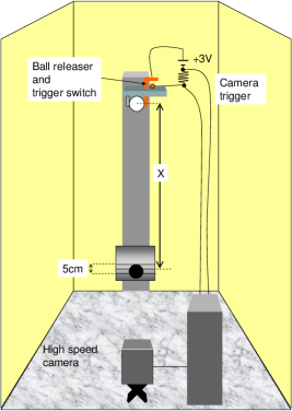
Figure 2: Experimental setup.

Snapshot S0 does not show the ball just released far above, outside the camera visual field. It is used only to determine the starting time. The whole system is triggered by a mechanic hook which simultaneously releases the ball and sends an electrical signal to the camera. Following the recorded images, one after the other on a computer screen, one sees nothing during many initial snapshots, while the ball is still above the camera visual field. However, the time is being counted every $(1/2000){\rm s}$. Suddenly, the ball appears inside the visual field, and one can observe the final part of its fall during half a hundred snapshots. Among them, snapshots S1 and S2 are chosen as described below.

Three horizontal lines were previously draw on a fixed dull glass plate illuminated from behind, in front of which the falling ball passes. Some four meters distant, the camera records the successive images. The height $X$ between the central line and the point where the ball was released is also previously determined. We used two recipes to choose snapshots S1 and S2 adopted as measures.

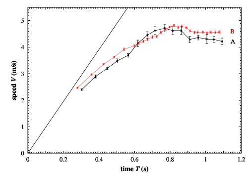
Figure 3: Directly measured speeds for a polystyrene ball with mass $m=0.22{\rm g}$ and diameter $D=2.47{\rm cm}$. Two superimposed experimental data sets were taken in different days. One with larger error bars and less points (A), converging to $V_{\ell}\approx 4{\rm m/s}$, taken during a hot Brazilian day (São Paulo), temperature around $30{\rm{}^{o}C}$. The other, with smaller error bars and more points (B), converging to a final speed close to $V_{\ell}\approx 4.5{\rm m/s}$, taken in a Brazilian normal day (São Paulo again), temperature around $25{\rm{}^{o}C}$. The previous measurements of figure 1 were made (with another ball of the same size) during a very hot Brazilian day (Rio de Janeiro), temperature $\approx 35{\rm{}^{o}C}$, $V_{\ell}=3.3{\rm m/s}$ measured in a much longer fall of $8.9{\rm m}$. The straight line corresponds to the free fall.

First, we took snapshot S1 when the ball enters into the central horizontal line, and S2 when the ball exits the same line. In this case, the distance to be divided by the time interval between snapshots S1 and S2 is the ball diameter itself. The result is one of the 5 speed measurements we repeat for each height, in order to average and to determine the error bars, figure 3, curve A.

Second, we took S1 as the snapshot when the ball exits the upper line, and S2 when it exits the bottom line. In this case, the distance to be divided by the time interval is the fixed distance between both lines, in our case $5.00{\rm cm}$. (Also in this case, the height $X$ in figure 2 is measured from the upper edge of the not-yet released ball.) For small balls ($D<5{\rm cm}$), this two-line option is more accurate than the previously described single-line approach. Also, for heights above $1.35{\rm m}$ when the turbulence effects appear, we made 10 instead of only 5 repeated measures. Furthermore, consecutive heights were taken closer, $10{\rm cm}$ instead of $20{\rm cm}$. The result is displayed in figure 3, curve B.

These experimental results agree with our preliminary conclusion concerning the ball decreasing speed after surpassing the final value $V_{\ell}$. We have done many other experiments with different balls, under the same or different weather conditions. During the same day when experiment (B) in figure 3 was performed, we have also observed the speed-decreasing behaviour for a smaller ball of diameter $D=2.02{\rm cm}$ and mass $m=0.14{\rm g}$, a little bit denser than the ball shown in figure 3. However, for a larger ball of diameter $D=3.04{\rm cm}$ and mass $m=0.35{\rm g}$ the decreasing speed effect was hardly visible. Larger yet balls of diameters $5{\rm cm}$ and $7{\rm cm}$ definitely do not show the same behaviour.

The results of another experiment with tiny balls falling in water [4] reinforce our conclusion. Although no speed above $V_{\ell}$ was observed for the glass or metallic balls used in this experiment, an oscillating speed was observed during the transient. First, the speed increases up to a certain value close to the future $V_{\ell}$, then decreases a litle bit, increases again and so on, eventually stabilising at $V_{\ell}$. The authors “expect the motion of a lighter bead to be more influenced by the eventual unsteadiness of its wake”[4]. Their interpretation for the speed oscillations is also linked to the “temporal evolution of the particle wake”. They also quote that “the oscillations disappear if the motion is averaged over several falls”, showing that “the events in the wake that are responsible for them are not coherent, in the sense that they do not occur at fixed times”. We can add that the wake formation is triggered by some minor early fluctuations occurred in the air around the ball, gradually amplified by the flow non-linear character. The triggering fluctuations naturally vary for different fall realisations.

After reaching $V_{\ell}$, the ball weight is equal to the drag force, leading to the relation $V_{\ell}^{2}=(4\,\rho_{ball}\,g\,D)/(3\,C_{D}\,\rho)$, where $C_{D}\approx 0.4$ or $0.5$ is the experimentally known drag coefficient almost constant for the range of Reynolds numbers relevant in our case. This is in perfect agreement with our final speeds $V_{\ell}\approx 4{\rm m/s}$. Moreover, by taking balls made of the same material (same $\rho_{ball}$), this relation shows that the final speed $V_{\ell}$ is smaller for smaller balls, also in agreement with our experiments. On the other hand, during the fall beginning the speed increases according to an acceleration close to $g$, independent of the ball size. Therefore, the initially increasing speed of smaller balls can surpass their small values of $V_{\ell}$. But larger balls do not, again in agreement with our experiments.

Another requirement is the ball weight (or density $\rho_{ball}$) which should be also small enough in order to allow a reasonable difference between the maximum speed and $V_{\ell}$. For another polystyrene ball with the same diameter as those in figures 1 or 3, but with a smaller mass of $0.14{\rm g}$ (the ball was cut into two hemispheres, the inner part was removed and the halves were glued again), we have observed the same decreasing speed behaviour, with both the maximum speed and $V_{\ell}$ smaller than those in figure 3. On the other hand, two other balls made of a denser polystyrene material ($D=2.02{\rm cm}$, $m=0.29{\rm g}$ and $D=1.50{\rm cm}$, $m=0.10{\rm g}$) soon reach their maximum speed ($\approx 6{\rm m/s}$ at $\approx 0.8{\rm s}$ and $\approx 5{\rm m/s}$ at $\approx 0.9{\rm s}$ respectively), but the speed decreasing after that is hardly noticeable due to the limiting height of $3.35{\rm m}$ inside the laboratory room. As $6{\rm m/s}$ and $5{\rm m/s}$ are already close to the expected values for their final speeds, probably the decreasing speed effect would not appear for these two balls. The direct measurement of $V_{\ell}$ through a much higher height, as we have done for the ball in figure 1, is impossible inside the laboratory room. Outside, on the other hand, it would be useless because the weather conditions would be modified. (All data in figure 1 as well as the value $V_{\ell}=3.3{\rm m/s}$ were obtained with a hand chronometer, instead of the sophisticated camera, at the same day and outside the laboratory room.)

A third important element is of course the weather itself. Different temperatures, atmospheric pressures, air humidity and density modify the air viscosity effects. Experiments inside the laboratory room with the air conditioner turned on (temperature $\approx 20{\rm{}^{o}C}$, air density, humidity and pressure not measured) also did not show the decreasing speed effect.

3 Phenomenological Support

Our experimental result and its interpretation can be summarised as follows. Released without initial speed, a small and light enough ball (diameter $D\approx 2.5{\rm cm}$ and mass $m\approx 0.2{\rm g}$, i.e. made of very low density material with at most $\approx 20$ times the air density) presents a maximum speed during its fall on air. Then, the speed decreases and reaches a smaller and constant value $V_{\ell}$, but only after a turbulent vortex wake is completely developed behind (above) the ball, the so-called von Kármán vortex street.

The crucial feature of our interpretation is the initial absence of the turbulent wake behind the ball, while its speed gradually increases. Can this scenario be confirmed through the solution of Navier-Stokes equations?

Some difficulties arise. The first one is a non-constant Reynolds number ${\cal R}=\rho\,V\,D/\eta$ in our case, different from traditional wind tunnel experiments where only the steady-state situation is measured with fixed $V$. Suppose we adopt a numerical approach, with $\Delta t=0.0025$ as the discrete time interval, in units of $D/V_{\ell}$: we would need some $6\times 10^{4}$ time steps in order to follow the first second of the fall. Considering one hour the processing computer time for each time step (a plausible estimate with single processors), the whole thing would spend 7 complete years.

This difficulty leads us to adopt some simplifications. First, to consider a fixed Reynolds number, say ${\cal R}=30$ or $1000$, but starting the solution at $t=0$ with the Stokes configuration of laminar air flow around the ball, previously obtained with ${\cal R}\to 0$ (or $V\to 0$). This would correspond not exactly to our experiment, but to an imaginary experiment realised in a wind tunnel initially kept off (air around the ball at rest) and suddenly turned on with a fixed wind speed. Our purpose is to observe only the first snapshots of the wake formation, far before the steady-state situation. In particular, we are interested in verifying the existence or not of some transient regime occurring before the turbulent wake with the endless formation of successive vortices appears.

Another simplification is to replace the ball by a long cylinder perpendicular to the air flow, supposing perpendicular to the cylinder all velocities in different points of the air around. This trick reduces our numerical effort from 3 to 2 dimensions. Indeed, according to many real experiments with a cylinder, the vortices are also cylindrical and parallel to it, with good accuracy, within the range of Reynolds numbers we are dealing with. Also the known experimental plots for the steady-state drag force as a function of the Reynolds number are completely equivalent, even quantitatively, for a ball or for a cylinder. All orders of magnitude are the same. In reality, reference [1] shows the experimental plots for a cylinder (see also the classical papers [5, 6]) and not for a ball, which can be found elsewhere (for instance [7, 2]).

Within the unusual but very interesting Feynman formulation, the Navier-Stokes equation reads

$$\frac{\partial{\vec{\omega}}}{\partial t}=\frac{1}{\cal R}\nabla^{2}\vec{\omega}-\vec{\nabla}\times(\vec{\omega}\times\vec{v})$$

where $\vec{v}$ are the air velocities in different positions.

The vorticities

$$\vec{\omega}=\vec{\nabla}\times\vec{v}$$

are auxiliary uni-dimensional vectors parallel to the cylinder. They are strategically located at the centres of each square plaquette of the $\vec{v}$ grid used for the numerical solution.

Moreover, air density fluctuations do not appear in our experiment because all speeds are much smaller than the sound speed ($\approx 330{\rm m/s}$). Therefore we can set

$$\vec{\nabla}\,\bullet\,\vec{v}=0\,\,\,\,.$$

The above Navier-Stokes equation is already written in an adimensional form, i.e. the cylinder diameter is $D=1$ and the wind speed (far from the cylinder and the wake) is $V=1$ pointing along the $X$ axis. In order to translate the results for normal units, one should simply adopt the real $D$ as the length unit and the real $V$ as the speed unit. Consequently, the time unit is $D/V$.

We solved this equation for the following boundary conditions. A rectangle is considered between $x=-3$ and $x=+7$, and between $y=-2.5$ and $y=2.5$, divided into $400\times 200$ pixels. Outside this rectangle, the wind speed is $V=1$ pointing along $X$. The cylinder axis coincides with $x=y=0$, and the speed is zeroed inside it, $x^{2}+y^{2}\leq(1/2)^{2}$. Between these two boundaries, two-dimensional velocities on the 80,000 grid points (the centre of each pixel) were determined numerically, through the above equations, as follows. Finite difference versions of the differential operators were used with second order accuracy, both in time and space. From one time step to the next, all $\vec{\omega}$ were relaxed in order to obey the $\nabla^{2}$ operator in the first equation, under fixed $\vec{v}$. After each (whole grid) $\vec{\omega}$ relaxation, corrected vectors $\vec{v}$ were determined from the other two equations applied to the fixed $\vec{\omega}$, by also relaxing all $\vec{v}$ some hundred times. Then, all $\vec{\omega}$ were relaxed again, and so on, until numerical convergence over the whole grid.

As far as we know, this numerical approach is new. We did not pay much attention to improve its computer time performance, a task postponed to the future. Many other methods are already adopted and optimised (mainly by engineers), including some very efficient commercial softwares [2]. Most of them are applied in order to study the steady-state regime. A few recent works treat the transient regimes [8], although all being very far from the specific case of our falling ball.

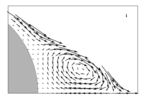
Figure 4: Successive snapshots showing the vortex formation behind a fixed cylinder (part of its grey back edge is shown on bottom left). Arrows represent local air velocities. Only a very small region behind the cylinder is shown, half a diameter downstream along the $X$ axis. Also, only points above the $X$ axis are shown, below it all velocities are mirror symmetric. Only very small speeds $V<0.007$ are represented. Downstream, much larger speeds $V\approx 1$ are omitted for clarity in the white (top right) part of the figures. The initial configuration (a) corresponds to the Stokes laminar flow ${\cal R}\to 0$ previously determined. Then, at $t=0$, the Reynolds number is suddenly turned on to ${\cal R}=30$. Time runs from figures (a) to (b), (c), etc, showing the gradual formation of the vortex we will call UP. The $X$ axis acts as a mirror, a second, symmetric vortex DOWN (not shown) spinning in the other sense is also simultaneously formed below each figure. For this small Reynolds number, these two vortices become eventually stuck at the position shown in the last figure, with negligible fluctuations around. For larger Reynolds numbers and after some time, however, each of these same two initial vortices alternately bifurcate, forming the long von Kármán vortex street (see text).

For a nice animation of the flow past a sphere, see [9]: the initial single vortex is a torus symmetric around the movement axis, which forms behind but near the ball. Afterwards, this symmetry is broken and the long turbulent wake with successive vortices develops, no longer torus-like. Returning back to the cylindrical symmetry we adopted in our numerical solution, figures 4a, 4b $\dots$ 4i show consecutive snapshots of the result for ${\cal R}=30$.

We have done the same for ${\cal R}=1000$ (not shown). The beginning is the same, two symmetric vortices, UP and DOWN, appear. The most noticeable difference is the (horizontally) stretched form of these vortices, instead of the rounded form shown in figure 4. Also, due to the stretching, they don’t remain stuck forever. After some time, one of them (UP in our computer run) bifurcates in two, forming a no longer symmetric wake with 3 vortices. Later, vortex DOWN also bifurcates, leading to 4 vortices, and so on. After some time, a very long wake of alternate vortices is dragged by the cylinder. Then, its contribution to the drag force becomes important.

In short, there are two different steady-state regimes. For small enough Reynolds numbers, only two symmetric vortices form and eventually stabilise at a fixed distance behind the cylinder. For large Reynolds numbers, instead of two vortices at rest, a many-vortices long wake is formed downstream, continuously fed with new vortices periodically appearing near the cylinder.

As a technical detail, for ${\cal R}=1000$ we have modified a little bit the boundary conditions at $x=7$. Instead of fixing $V=1$ outside, we copy the rightmost column of velocities still inside the rectangle to the next column already outside. Then, for the next time step, we fix this column with velocities which are weighted averages between this copy and $V=1$, taking the averaging weights for the copy proportional to the distance to the $X$ axis (zero weight at $y=\pm 2.5$, unit weight at $y=0$). This artificial trick allows the wake to escape through the back door, but certainly also introduces some unknown perturbation on the wake after many vortices were already escaped. Even so, we could observe the formation of many new vortices, not yet in the steady state regime within our limited computer time. This unknown influence of the boundary conditions, however, is not important here because we are interested only in the beginning of the process, with only the first two symmetric vortices, when one of them bifurcates still inside the rectangle ($x\approx 3$ for ${\cal R}=1000$).

For a would-be gradually increasing-${\cal R}$ numerical solution, we can foresee the following scenario. First, only two symmetric vortices stabilises for a while into a position initially very near the cylinder. Then, as the Reynolds number increases, these vortices become stretched, and their centres reach regions farther and farther behind the cylinder, but still symmetric and at rest (completely dragged by the cylinder). Suddenly, a rupture occurs: one of the vortices bifurcates in two, then the other, and so on, triggering the construction of a continuously-fed turbulent wake of vortices slowly moving downstream. Only after this rupture, the friction force starts to become important.

This scenario is qualitatively compatible with our polystyrene falling ball experiment. Although the many-vortices wake is already observed in our numerical solution for a fixed ${\cal R}=1000$, we could expect the triggering rupture to occur somewhat later within the (unfeasible) gradually increasing-${\cal R}$ solution, where the first two symmetric vortices would have time enough to (meta) stabilise themselves under the previously smaller Reynolds numbers. Slow, adiabatic stretching is naturally more resistant against rupture than the sudden stretching we tested by switching ${\cal R}=0$ directly to ${\cal R}=1000$ at $t=0$. So, the scenario obtained from the phenomenological Navier-Stokes equation can be also quantitatively compatible with our experiment.

4 Conclusions

By measuring the successive speeds of a polystyrene ball falling on air, initially released from a certain height, we could observe a completely unexpected behaviour: the ball reaches a maximum speed, then breaks, and finally a limit speed $V_{\ell}$ is stabilised, as expected. We found two conditions as necessary in order to observe this. First, the ball should be light enough in order to allow a small value for $V_{\ell}$ (in our case, $V_{\ell}\approx 4{\rm m/s}$). Second, the ball should be small enough (in our case, diameter $D\approx 2.5{\rm cm}$ or less).

Our interpretation is based on the transient time before the development of the so-called von Kármán vortex street of air vortices behind (above) the ball. This long wake of vortices (some hundred diameters) is the responsible for the drag force which eventually compensates the gravitational attraction exerted by Earth on the ball, providing its final constant speed $V_{\ell}$. Before the wake development, under a smaller dragg force, the ball can reach speeds larger than $V_{\ell}$, because this limit will be imposed only after the “infinite” wake is already developed.

Numerical solutions of the phenomenological Navier-Stokes equations for a cylinder give support to our interpretation. The turbulent wake consists of the periodic creation of new vortices which slowly move downstream one after the other, the same scenario observed in steady-state wind tunnel experiments. However, starting with zero speed, our numerical solutions show another transient regime holding before the wake formation. First, just two symmetric vortices form and become stuck for a while, characterising the quoted transient. Suddenly, one of them bifurcates, forming a third vortex, then the other suffers the same process, starting the formation of the eventual many-vortices wake.

For spheres instead of cylinders, a single torus-like vortex forms behind the sphere at first, and stays dragged by the sphere for a while. Suddenly, it breaks down into a sequence of successive, no-longer torus-like vortices which go away along the street. We deal with a rupture phenomenon, a transition between an initial regime where a symmetric vortex stays for a while at rest relative to the ball, towards a second regime where a sequence of successive non-symmetric vortices move away from the ball.

Besides the speed decreasing curious behaviour, maybe this naive experiment could shed light in some transient and hysteresis phenomena occurring within fluid dynamics, a subject not very well known.

References

- [1] R.P. Feynman, The Feynman Lectures on Physics, vol. II, chap. 41, Addison-Wesley, Reading, Massachusetts (1965).
-
[2]
D.A. Jones and D.B. Clarke, http://dspace.dsto.defence.gov.au
/dspace/bitstream/1947/9705/1/DSTO-TR-2232 PR.pdf. - [3] G. Feinberg, Am. J. Phys. 33, 501 (1965); C.G. Adler and B.L. Coulter, Am. J. Phys. 46, 199 (1978); B.L. Coulter and C.G. Adler, Am. J. Phys. 47, 841 (1979).
- [4] M. Mordant and J.-F. Pinton, Eur. Phys. J. B18, 343 (2000).
- [5] M. Provansal, C. Mathis and L. Boyer, J. Fluid Mech. 182, 1 (1987).
- [6] C.H.K. Williamson, Phys. Fluid 31, 3165 (1988).
- [7] I. Nakamura, Phys. Fluids 19, 5 (1976).
- [8] N. Abdessemed, A.S. Sharma, S.J. Sherwin and V. Theofilis, Phys. Fluids 21, 044103 (2009); L.Q. Wang, Z.F. Li, D.Z. Wu and Z.R. Hao, Int. J. Comp. Fluid Dyn. 21, 127 (2007); H.M. Blackburn and S.J. Sherwin, J. Fluid Mech. 573, 57 (2007); M.S. Engelman and M.-Ali Jammia Int. J. Num. Meth. Fluids 11, 985 (2005); J. Hoepffner, L. Brandt and D.S. Henningson, J. Fluid Mech. 537, 91 (2005); S.J. Sherwin and H.M. Blackburn, J. Fluid Mech. 533, 297 (2005); F. Sy, J.W. Tauton and E.N. Lightfoot, AIChE J. 16, 386 (2004); N. Kensei, K. Teruhiko, K. Mitsuo, Y. Zensaburo and T. Hirokazu, Trans. Japan Soc. Mech. Eng. B69, 53 (2003).
- [9] www3.icfd.co.jp/examples/SPHERE/SP1.HTM, and references therein by K. Kuwahara, S. Komurasaki and others.