Smoothly-Rising Star Formation Histories During the Reionization Epoch

Abstract

Cosmological hydrodynamic simulations robustly predict that high-redshift galaxy star formation histories (SFHs) are smoothly-rising and vary with mass only by a scale factor. We use our latest simulations to test whether this scenario can account for recent observations at $z\geq 6$ from WFC3/IR, NICMOS, and IRAC. Our simulations broadly reproduce the observed ultraviolet (UV) luminosity functions and stellar mass densities and their evolution at $z=6$–8, all of which are nontrivial tests of the mean SFH. In agreement with observations, simulated galaxies possess blue UV continua owing to young ages (50–150 Myr), low metallicities (0.1–0.5$Z_{\odot}$), and low dust columns ($E(B-V)\leq 0.05$). Our predicted Balmer breaks at $z=7$, while significant, are $\approx 0.5$ magnitudes weaker than observed even after accounting for nebular line emission, suggesting observational systematic errors and/or numerical resolution limitations. Observations imply a near-unity slope in the stellar mass–star formation rate relation at all $z=6$–8, confirming the prediction that SFH shapes are invariant. Dust extinction suppresses the UV luminosity density by a factor of 2–3, with suppression increasing modestly to later times owing to increasing metallicities. Current surveys detect the majority of galaxies with stellar masses exceeding $10^{9}M_{\odot}$ and few galaxies less massive than $10^{8.5}M_{\odot}$, implying that they probe no more than the brightest $\approx 30\%$ of the complete star formation and stellar mass densities at $z\geq 6$. Finally, we demonstrate that there is no conflict between smoothly-rising SFHs and recent clustering observations. This is because momentum-driven outflows suppress star formation in low-mass halos such that the fraction of halos hosting observable galaxies (the “occupancy”) is 0.2–0.4 even though the star formation duty cycle is unity. This leads to many interesting predictions at $z\geq 4$, among them that (1) optically-selected and UV-selected samples largely overlap; (2) few galaxies exhibit significantly suppressed specific star formation rates; and (3) occupancy is constant or increasing with decreasing luminosity. These predictions are in tentative agreement with current observations, but further analysis of existing and upcoming data sets is required in order to test them more thoroughly.

1 Introduction

In the era of precision cosmology, the study of galaxy evolution is an initial value problem in which the goal is to characterize the processes that connect the initial conditions at $z\approx 1090$ (for example, Komatsu et al., 2010) to galaxies, which had evidently begun forming by $z=10$ (for example, Stark et al., 2007; Bouwens et al., 2009c; Yan et al., 2009). The initial-value nature of the problem implies that detailed measurement of its earliest stages constitutes an immensely useful aid through its ability to anchor an understanding of the later stages. Gas inflows, outflows, and other feedback processes impact high-redshift star formation histories (SFHs). Hence observational inferences regarding the SFHs at high redshift constrain star formation and feedback both at early times and at subsequent epochs.

Cosmological hydrodynamic simulations robustly predict smoothly-rising SFHs (Finlator et al., 2007) with a scale-invariant shape at $z\geq 6$. Therefore, any comparison between simulation predictions and observations constitutes a (possibly indirect) test of this scenario. We have previously demonstrated considerable success in using cosmological hydrodynamic simulations to interpret observations of high-redshift galaxies. In Finlator et al. (2006), we showed that simulations of a $\Lambda$CDM universe with star formation modulated by outflows with a constant wind speed and mass loading factor broadly reproduce the observed rest-frame UV luminosity function (LF) at $z\sim 4$. We confirmed previous numerical predictions (for example, Davé et al., 2000; Weinberg et al., 2002) that stellar mass ($M_{*}$) and star formation rate (SFR) correlate, finding a small scatter and a slope near unity. A qualititatively similar correlation has now been observed at all redshifts out to $z=7$ (Brinchmann et al., 2004; Elbaz et al., 2007; Noeske et al., 2007a; Daddi et al., 2007; Salim et al., 2007; Schiminovich et al., 2007; Pannella et al., 2009; Labbé et al., 2009; Bothwell et al., 2009; Oliver et al., 2010; Magdis et al., 2010), although observations at $z<2$ tend to suggest a somewhat flatter slope of 0.7–0.9 that is associated with galaxy downsizing (Brinchmann et al., 2004; Elbaz et al., 2007; Noeske et al., 2007a; Daddi et al., 2007; Salim et al., 2007; Schiminovich et al., 2007; Bothwell et al., 2009; Magdis et al., 2010). This correlation has two implications: First, it implies that UV-selected galaxies are generically the most massive (star-forming) galaxies at a given redshift (Nagamine et al., 2004; Finlator et al., 2006) unless the scatter is quite large (Weinberg et al., 2002). Second, a slope of unity supports a scenario in which SFHs have a scale-invariant shape such that, on average, galaxies’ SFHs differ only by a scale factor. The SFR-$M_{*}$ relation therefore constitutes a key prediction of galaxy evolution models (for example, Bouché et al., 2009; Dutton et al., 2009). We additionally predicted that high-redshift galaxies should exhibit pronounced Balmer breaks because smooth SFHs naturally yield evolved stellar populations. With the arrival of rest-frame optical constraints from IRAC, this prediction has now received dramatic confirmation (for example, Bradley et al., 2008; Chary, Stern & Eisenhardt, 2005; Dow-Hygelund et al., 2005; Dunlop et al., 2007; Egami et al., 2005; Eyles et al., 2005, 2007; Labbé et al., 2006; Lai et al., 2007; Labbé et al., 2009; Stark et al., 2009; Verma et al., 2007; Yan et al., 2005; Pentericci et al., 2009; Zheng et al., 2009), although the question of whether emission lines could be mimicking the observed Balmer breaks remains unresolved (Schaerer & de Barros, 2009, 2010).

In Davé et al. (2006, hereafter DFO06), we tested a treatment for momentum-driven outflows from star-forming regions against the available constraints on the rest-frame UV and Ly$\alpha$ LFs at $z\sim 6$, finding reasonable agreement in both cases. This result was subsequently extended by Bouwens et al. (2007), who found that our simulation’s prediction for the evolution of the UV LF normalization from $z=8\rightarrow 4$ was well-matched by observations. This is a nontrivial test of our predicted SFHs because constant or decaying SFHs would predict a different evolution of the UV LF than is observed.

Finally, in Finlator et al. (2007), we showed that our simulations could account for the rest-frame UV-to-optical spectral energy distributions (SEDs) of 5 out of 6 observed galaxies between $z=5.5$–6.5. We demonstrated that smoothly-rising SFHs are equally as plausible as more popular constant or exponentially-decaying models. We then used these comparisons to explore the implied physical properties such as SFR, $M_{*}$, and age, finding good agreement with previous constraints although with significantly narrower posterior probability distributions owing to the tight priors imposed by the physical correlations that our simulations predict.

While these studies are encouraging, their support for our SFH scenario is somewhat indirect because, until recently, observations at $z\geq 6$ did not clearly imply a unique SFH. For example, any galaxy evolution model that predicted scale-invariant SFH shapes would predict an SFR-$M_{*}$ relation with a slope of unity. Similarly, any SFH shape can be tuned to reproduce the observed UV LF at one epoch, and bursty SFHs could be tuned to reproduce it at multiple epochs. The fundamental difficulty is that broadband SEDs do not contain enough information to constrain the underlying SFHs of individual objects, even when analyzed through detailed SED-fitting studies (for example, Shapley et al., 2001; Papovich et al., 2001).

Since the completion of these previous works, a number of authors have used new data from the HST WFC3/IR and NICMOS cameras as well as Spitzer/IRAC to increase the number of objects at $z\geq 6$ with published rest-frame UV to optical constraints (Bouwens et al., 2009b, 2010a; Bunker et al., 2009; Castellano et al., 2009; Finkelstein et al., 2009; Gonzalez et al., 2009; Labbé et al., 2009, 2010; McLure et al., 2010; Oesch et al., 2010a, b; Ouchi et al., 2009; Yan et al., 2009). Using these new samples, we may now ask whether the mean SFH of reionization-epoch galaxies is constrained even if individual SFHs are not. For example, Stark et al. (2009) recently pointed out that the observed lack of evolution in the specific star formation rate (SSFR) of UV-selected galaxies from $z=$4–6 (see also Overzier et al., 2009; Gonzalez et al., 2009) rules out the possibility that the majority of galaxies observed at $z=4$ have been forming stars at constant or declining rates since $z\geq 5$. This is because constant or declining SFHs would predict higher SSFRs at earlier times, in conflict with their observations. They noted that smoothly-rising SFHs could explain their observations since in this case galaxies would grow in $M_{*}$ and SFR simultaneously.  Papovich et al. (2010) studied the evolution of the UV luminosity and stellar mass at constant number density and concluded that observations require smoothly-rising SFHs and are consistent with a scale-invariant shape from $z=8\rightarrow 3$. Finally, Maraston et al. (2010) argued in favor of exponentially-rising over decaying SFHs as models for star-forming galaxies at $z\sim 2$ for two reasons. First, they found that rising SFHs provide better fits both to observations and to predictions from semi-analytic models of galaxy formation. Second, rising SFHs naturally explain higher-redshift samples as the fainter progenitors of lower-redshift samples.

These suggestions exemplify how statistical samples at multiple epochs can constrain the mean SFH even if the SFHs of individual galaxies are unconstrained. In this work, we use this idea to build upon the results of Finlator et al. (2007) by asking whether smoothly-rising SFHs can explain the observed statistical properties of galaxies at $z=6$–8. Broadly, since all of our simulated high-redshift galaxies experience smoothly-rising SFHs, any comparison with observations can be viewed as an indirect test of these models. In most cases, however, the constraining power of large samples at multiple epochs will render our comparisons direct tests of the smoothly-rising scenario.

We describe our simulations in Section 2. In Section 3, we review the rising SFH scenario and summarize its predictions. We compare our predicted UV LFs with observations in Section 4. We perform detailed comparisons between simulated and observed SEDs in Section 5. Additionally, we use our simulations to predict the completeness of current $z\geq 6$ surveys. In Section 6, we study the predicted relationships between stellar mass, star formation rate, star formation history, and metallicity, comparing with observations where possible. In Section 7, we use our predicted halo occupation distribution to argue that recent clustering observations are consistent with smooth SFHs, and we discuss further tests of our model and alternative bursty SFH scenarios. In Section 8, we comment on processes that cause SFHs to depart from our smoothly-rising, scale-invariant scenario at lower redshift. Finally, we summarize our results in Sec 9.

2 Simulations

2.1 Numerical Simulations

Table 1: Simulation parameters.

$L$	$\epsilon$	$m_{\rm SPH}$	$m_{\rm dark}$	$M_{\rm*,min}$
$12$	$0.469$	$0.235$	$1.19$	$15.0$
$24$	$0.938$	$1.87$	$9.55$	$120$
$48$	$1.88$	$15.0$	$76.4$	$962$

We ran our cosmological hydrodynamic simulations using our custom version of the parallel cosmological galaxy formation code Gadget-2 (Springel & Hernquist, 2002; Springel, 2005). This code uses an entropy-conservative formulation of smoothed particle hydrodynamics (SPH) along with a tree-particle-mesh algorithm for handling gravity. It accounts for photoionization heating starting at $z=9$ via a spatially uniform photoionizing background (Haardt & Madau, 2001). Gas particles undergo radiative cooling under the assumption of ionization equilibrium, where we account for metal-line cooling using the collisional ionization equilibrium tables of Sutherland & Dopita (1993).

The assumption of ionization equilibrium with a uniform ionizing background may become increasingly inappropriate as we push our predictions beyond $z=6$, where cosmological reionization is believed to have ended (for example, Fan et al., 2006). We argued in DFO06 that the observable galaxies at $z=6$–10 live in sufficiently biased regions that their environments were probably reionized early relative to the cosmological mean, with the implication that the Haardt & Madau (2001) ionizing background is not a strong approximation. In future work, we will relax this assumption through self-consistent radiative hydrodynamic simulations. However, we retain it in our present work for simplicity, in essence adding this to the list of approximations that our comparisons test.

We endow dense gas particles with a subgrid two-phase interstellar medium consisting of hot gas that condenses via a thermal instability into cold star-forming clouds, which are in turn evaporated back into the hot phase by supernovae (McKee & Ostriker, 1977). The model requires only one physical parameter, the star formation timescale, which we tune in such a way that it reproduces the Kennicutt (1998a) relation (Springel & Hernquist, 2003).

We have improved our treatment of the formation and transport of metals. We summarise these changes here; for details we refer the reader to Oppenheimer & Davé (2008). Star-forming gas particles self-enrich owing to Type II supernovae as before, but we now incorporate the metallicity-dependent Type II supernova yields from Chieffi & Limongi (2004) assuming a Chabrier (2003) IMF. We account for mass loss from AGB stars using the delayed feedback tables of Bruzual & Charlot (2003). We account for energy and metal feedback from Type Ia supernovae (both prompt and delayed populations). Finally, we track the enrichment rates of C, O, Si, and Fe separately rather than tracking only the total metal mass fraction. Gas particles stochastically spawn star particles via a Monte Carlo algorithm in such a way that the growth of stellar mass in star particles reflects the underlying star formation rate in the gas particles. Each star particle inherits the metallicity of its parent gas particle.

Galaxy formation models must invoke galactic-scale outflows in order to avoid the overcooling problem (White & Frenk, 1991). We have previously shown that models coupling the outflow speed and mass-loading factor (that is, the mass of material expelled per unit mass of stars formed) to the halo mass are uniquely successful in reproducing a wide variety of observations of galaxies (Davé et al., 2006; Finlator & Davé, 2008; Oppenheimer et al., 2010), and the IGM (Oppenheimer & Davé, 2006, 2008, 2009a; Oppenheimer et al., 2009b). In this work, we again use momentum-driven outflows with a normalization $\sigma_{0}=150\;{\rm km}\,{\rm s}^{-1}$. In order to improve the fidelity with which we implement momentum-driven outflow scalings, we now compute mass loading factors using the velocity dispersion of each gas particle’s host galaxy rather than the local gravitational potential. The velocity dispersion is in turn computed from the host galaxy’s baryonic mass using Mo et al. (1998). For further details on the physics treatments in the simulations, see Oppenheimer & Davé (2006, 2008); Oppenheimer et al. (2010).

Our fiducial simulation volume is a cube $24h^{-1}{\rm Mpc}$ long on each side that uses $512^{3}$ dark matter and star particles. With a mass resolution limit of 128 star particles, this implies that our fiducial volume resolves stellar populations more massive than $1.20\times 10^{8}M_{\odot}$. This mass limit translates into a limiting UV magnitude via the simulated star formation histories (SFHs) and the assumed stellar population synthesis model; we will show in Section 4 that this resolution limit is well-matched to current observational limits. Throughout this work, we will evaluate resolution convergence by comparing with results from additional simulations whose volumes span $12$ and $48h^{-1}{\rm Mpc}$ with the same number of particles, for an implied stellar mass resolution limit of $1.50\times 10^{7}M_{\odot}$ at our highest resolution (see Table 1).

We assume a cosmology where $\Omega_{M}=0.28$, $\Omega_{\Lambda}=0.72$, $H_{0}=70\;{\rm km}\,{\rm s}^{-1}\;{\rm Mpc}^{-1}$, $\sigma_{8}=0.82$, and $\Omega_{b}=0.046$. Note that we do not correct observed photometry to our assumed cosmology because the implied corrections are typically small ($\approx 0.05$ mag) compared to the uncertainty inherent in photometric redshifts ($\approx 0.2$ mag). We measure simulated UV luminosities using a narrow boxcar filter at 1350 Å that is not contaminated by Lyman-$\alpha$ emission or absorption by the intergalactic medium along the line of sight, and we do not $k$-correct observed UV luminosities to 1350 Å because these corrections are also small.

2.2 Identifying Simulated Galaxies

We identify galaxies within our simulations as gravitationally-bound lumps of star and gas particles using SKID (see Kereš et al. 2005 for a description). We sum the SFRs over each galaxy’s gas particles to obtain its instantaneous SFR. We obtain its star formation history by examining the ages of its star particles. We compute its stellar metallicity by performing a mass-weighted average over its star particles. We define its gas metallicity as the SFR-weighted mean metallicity over its gas particles in order to mimic the metallicities that would be measured from its emission lines if this were possible. In detail, our use of the mass-weighted stellar metallicity may not be completely appropriate for comparison with high-redshift observations given that the observed luminosities are dominated by the youngest stars. However, we will justify this choice in Figure 11 by showing that the SFR-weighted gas metallicity, which dictates the metallicity of the most luminous stars in each galaxy, typically exceeds the mass-weighted stellar metallicity by only 0.2 dex.

Note that we use SKID to identify the galaxies at each redshift snapshot independently. This means that our analysis does not depend on our ability to identify each galaxy’s progenitors and descendants (except for the illustrative evolutionary trends in Figures 10 and 11). Consequently, we refer the “SFH” at a given epoch to the stellar age distribution, independent of whether those stars formed in-situ or in smaller progenitors that were accreted at earlier times. While this approach prevents us from studying our simulated merger histories, Guo & White (2008) have shown that mergers are expected to be subdominant in modulating the SFHs of high-redshift galaxies (see also Cattaneo et al. 2010). The generally smooth SFHs predicted by our model support this view.

We obtain each simulated galaxy’s stellar continuum by convolving its stellar population with the Bruzual & Charlot (2003) stellar population synthesis models assuming a Chabrier (2003) initial mass function (IMF) and the ’Padova 1994’ stellar evolution models (see Bruzual & Charlot 2003 for references), interpolating within the tables to the correct metallicity and age for each star particle. We account for dust using the foreground screen model of Calzetti et al. (2000), where each galaxy’s assumed reddening $E(B-V)$ is tied to the mean stellar metallicity using a local calibration (Finlator et al., 2006). We treat the effect of absorption by the intergalactic medium (IGM) along the line of sight to each galaxy using Madau (1995). Finally, we convolve the resulting synthetic spectra with the appropriate photometric filter response curves to produce synthetic photometry. We have explicity checked that our photometry is unaffected when we use the updated population synthesis models of Charlot & Bruzual (2007) rather than Bruzual & Charlot (2003). This is expected because the observed Spitzer/IRAC [3.6] flux is not sensitive to the contribution of thermally pulsating asymptotic giant branch stars at redshifts greater than 6 (see also Stark et al., 2009; Labbé et al., 2010). Note that, throughout this work, we use $[3.6]$ and $[4.5]$ to denote Spitzer/IRAC Channels 1 and 2, respectively, and we use $Y_{105}$, $J_{125}$, and $H_{160}$ to denote the WFC3/IR F105W, F125W, and F160 bands, respectively.

In an improvement over our previous work, we now add nebular line emission to our simulated spectra before accounting for dust and the IGM opacity following Schaerer & de Barros (2009). We first compute the ionizing continuum luminosity directly from the stellar continuum, which automatically accounts correctly for the self-consistently predicted stellar population age and metallicity. We then compute the luminosity in all hydrogen recombination transitions from an upper state with $n\leq 50$ using Storey & Hummer (1995). This step involves several assumptions. First, we use Case B recombination theory and omit Lyman-$\alpha$. Second, we assume an electron density $n_{e}=100$ cm^-3 and temperature $T_{e}=10^{4}$K. This is representative because the luminosities vary by $\leq 30\%$ in the range $n_{e}=10^{2}$–$10^{4}$ cm^-3 and $T_{e}=$1000–30,000K. Finally, we follow Schaerer & de Barros (2010) in assuming that all ionizing photons are absorbed by hydrogen rather than dust. We then add the dominant allowed and forbidden metal lines using Anders & Fritze-v. Alvensleben (2003), interpolating linearly to each simulated galaxy’s metallicity. Incorporating emission lines in this way allows us to make physically-motivated predictions regarding the impact of emission lines on observable galaxies at $z\geq 6$.

The most uncertain aspect of our treatment for nebular emission involves the choice of ionizing escape fraction $f_{\mathrm{esc}}$. Optimally, one would like to constrain $f_{\mathrm{esc}}$ observationally, but current data do not permit this (Ono et al., 2010). We adopt the assumption that $f_{\mathrm{esc}}=0$ because it yields an upper bound to the effect that nebular emission can have on galaxy spectra. This is equivalent to assuming that current $z\geq 6$ samples did not bring about cosmological reionization. However, we will also argue that current samples probe only the brightest $1/3$ of all star formation at $z\geq 6$ anyway, hence this assumption is not inconsistent with the view that star formation dominated the reionization photon budget.

3 Rising Star Formation Histories

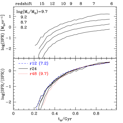
Figure 1: Simulated mean SFHs down to $z=5.5$ in four bins of stellar mass. Top: Mean star formation rates in galaxies whose stellar masses $\log(M_{*}/M_{\odot})$ at $z=5.5$ are, from bottom to top, 8.2, 8.7, 9.2, and 9.7. Bottom: The same SFHs but normalized to the respective mean SFRs. Our simulations predict that SFHs at early times are smoothly rising and vary only by a scale factor. Here we include representative normalized mean SFHs from our comparison volumes from galaxies with the indicated stellar masses. The good agreement with the SFHs from our r24 volume suggests that our mean SFH is numerically converged.

The goal of the current work is to test two fundamental predictions of our galaxy evolution model:

1. SFHs at early times are smoothly-rising (Finlator et al., 2007); and

2. SFH shapes are scale-invariant.

We illustrate these predictions in Figure 1. The top panel shows the mean simulated SFHs in four bins of stellar mass. We have generated these SFHs directly from the stellar age distributions of our simulated galaxies at $z=6$. These curves immediately demonstrate that SFHs are on average smoothly-rising prior to $z=6$. The growth timescale $t_{0}$ in an exponential fit of the form $\dot{M}_{*}\propto e^{t/t_{0}}$ evolves rapidly from 50 Myr at $z=12$ to 350 Myr by $z=6$.

The top panel strongly suggests that mean SFHs of simulated galaxies of different masses vary only by a scale factor. We demonstrate this second prediction explicitly in the bottom panel. Here, we have normalized each SFH by its mean SFR, which is just the total stellar mass formed by that SFH at $z=6$ divided by the age of the universe at $z=6$. The normalized mean simulated SFHs are nearly identical, especially after $z=12$. This implies that galaxy ages (and hence colours) should vary only weakly with luminosity, and that rest-frame optical and UV luminosities (or, equivalently, the inferred stellar mass and star formation rate) should correlate with a slope of unity.

This self-similarity may be surprising for two reasons. First, star formation is expected to be quenched at low masses owing to photoionization feedback and at high masses owing to the onset of hot-mode accretion, hence self-similarity cannot extend to arbitrarily low and high masses. Our simulations are sensitive to these effects because they include an optically-thin ionizing background and model the formation of virial shocks in halos. However, photoheating only suppresses star formation in halos less massive than $\sim 10^{8}M_{\odot}$ (Thoul & Weinberg, 1996; Okamoto et al., 2008) while virial shocks only suppress inflows in halos more massive than $10^{12}M_{\odot}$ (Kereš et al., 2005; Dekel & Birnboim, 2006; Kereš et al., 2009). The host halos of observed galaxies at $z\geq 6$ fall largely between these scales (Figure 13), hence they do not probe the processes that cause departures from self-similarity.

Second, it is surprising that galaxy age should be independent of mass because more massive dark matter halos are expected to have assembled more recently at any redshift (Lacey & Cole, 1993). This might lead one to expect more massive galaxies to be younger. However, Neistein et al. (2006) have shown that more massive dark matter halos are younger than less-massive halos only if each halo’s age refers to the epoch at which its most massive progenitor assembles half of the current mass. By contrast, if one identifies the halo age with the epoch at which more than half of the current mass has been assembled into all progenitors more massive than a given threshold, then the trend reverses and more massive halos are older. The stellar age distribution relates more closely to the latter age definition if star formation is inevitable in halos more massive than, for example, $10^{8}M_{\odot}$, hence one might equally expect galaxies in more massive halos to be older. However, the assembled mass fraction in all progenitors at a given redshift depends more weakly on mass than the mass fraction in the main progenitor (Figures 3 and 4 of Neistein et al. 2006). This means that the actual dependence of SFH on mass is likely to be driven by feedback processes such as outflows rather than reflecting underlying trends in halo assembly histories. For example, the momentum-driven wind scenario ties the outflow mass-loading factor to the circular velocity, which in turn varies as $H(z)^{1/3}$ (Mo et al., 1998); this could delay early star formation in massive halos enough to remove the downsizing trend in halo formation histories.

Numerical star formation histories suffer from resolution limitations at early times when the number of gas particles in the protogalaxies is small. Close inspection of the bottom panel of Figure 1 reveals that the normalized SFHs exhibit larger scatter at $z>12$, which probably reflects resolution effects. For this reason, it is important to test how sensitive our predicted mean SFH is to the simulation’s mass resolution. The blue dashed and red dotted curves in the bottom panel illustrate normalized SFHs drawn from our higher- and lower-resolution comparison volumes, respectively. They are in reasonable agreement with the mean SFHs predicted by our fiducial volume. This suggests that our predicted mean SFH is not strongly sensitive to numerical resolution effects. Moreover, given that the SFHs appear converged at $z<12$ and that most of the stars observed during $z=6$–8 formed after $z=12$, the early lack of convergence does not significantly affect our results. For reference, the mean SFHs in the bottom panel are well-fit by the following polynomial (where $t$ is the age of the Universe in Gyr):

$$\dot{M}_{*}\propto\left\{\begin{array}[]{ll}0&\mbox{if $t<0.27$}\\ 0.2-3.2t+10.5t^{2}-3.9t^{3}&\mbox{otherwise}\end{array}\right.$$ (1)

4 Luminosity Functions

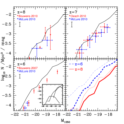
Figure 2: Observed (coloured points) and simulated (black) rest-frame UV LFs at z=6–8. The observed LFs are taken from McLure et al. (2010) and Bouwens et al. (2009b) at $z=8$; Oesch et al. (2010a) and McLure et al. (2010) at $z=7$; and Bouwens et al. (2007) and McLure et al. (2009) at $z=6$. The aggregate LFs are compiled from our three simulation volumes following DFO06; the inset panel in the bottom-left panel shows the three full LFs. Error bars show the jackknife error at $M_{\mathrm{UV}}=-19$ at each epoch; this includes Poisson uncertainty and cosmic variance. Predictions include dust extinction following Finlator et al. (2006). The simulations and observations agree to within a factor of 3 at all redshifts, suggesting that our star formation and feedback prescriptions adequately model galaxy evolution in the late reionization epoch. The lower heavy and upper light curves in the bottom-right panel show the simulated LF with and without dust reddening, respectively. The impact of dust is weak owing to low metallicities, and it grows progressively weaker with increasing redshift.

In the top-left, top-right, and bottom-left panels of Figure 2, we compare the simulated rest-frame 1350 Å LF with the observed UV LFs at redshifts 6–8. Before we discuss these comparisons, we note that our predicted LFs are uncertain owing to Poisson errors, cosmic variance, numerical resolution effects, and the choice of IMF. We estimate the contribution of Poisson errors and cosmic variance using jackknife resampling and show the resulting uncertainties at a representative absolute magnitude of $M_{1350}=-19$ in each panel; this is typically 20–30%. We estimate the impact of numerical effects by comparing the predicted LFs from our three volumes at $z=6$ in the inset panel; lower-resolution volumes typically overproduce the LF normalization by $\sim 50\%$. Finally, our choice of the Chabrier (2003) IMF yields luminosities $50\%$ brighter for the same stellar mass than we would find from the Salpeter (1955) IMF.

The normalizations of our predicted LFs agree with observations to within a factor of three at all three redshifts, which is generally within the combined theoretical and observational uncertainties. In particular, both the simulated and the predicted LFs may be regarded as brightening by 0.6–0.8 magnitudes during $z=8\rightarrow 6$. This is a nontrivial test of the smoothly-rising SFH scenario. To see this, note that, if the average star-forming galaxy at $z=6$ had been forming stars at a smoothly constant or declining rate since it formed, then the LF would be constant or grow dimmer to lower redshifts. Instead, observations strongly suggest that objects at constant number density grow brighter with time, implying that they increase their SFRs even as they increase their stellar masses (Papovich et al., 2010). This is the smoothly-rising SFH scenario. The predicted evolution probes the shape of the mean SFH, and the good agreement with observations suggests that the simulated SFH shape is realistic. Note that this interpretation depends on the assumption that SFHs are smooth rather than, for example, stochastically brightening into and then fading out of observed samples (Lee et al., 2009; Stark et al., 2009); we will argue on observational grounds that the SFHs are indeed smooth in Section 7.

While the normalization and its evolution are in reasonable agreement with observations, our simulations predict rather steep faint-end slopes $\alpha\approx-2.0$. This is similar to the slope of the halo mass function, hence our model predicts that low-mass halos possess a fairly constant star formation efficiency (defined as the ratio of the SFR to the gas mass). Observations indicate a somewhat shallower slope of $\approx-1.7$ at $z=6$ (for example, Bouwens et al., 2007), which could suggest that outflow strengths (or other feedback processes) scale more steeply with mass in reality than in our simulations. By contrast, observations at $z=$7–8 indicate a steeper faint-end slope of $\approx-2$ (Bouwens et al., 2010b), in better agreement with our predictions. If this evolution is confirmed, it could indicate that the feedback process that flattens the faint end of the LF at $z\leq 6$ is overwhelmed by the high gas inflow rate at earlier times, as expected in a scenario where the star formation and outflow rates do not “catch up” to the inflow rate until later times (Bouché et al., 2009; Papovich et al., 2010).

Figure 3: The predicted relationship at $z=7$ between dust reddening and stellar mass (top) and absolute UV luminosity including the dust (bottom). The three loci in each panel reflect our three simulation volumes. Typical colour excesses of 0.05 are predicted at all luminosities, although a fraction of galaxies more luminous than $M_{UV}<-19$ are predicted to have $E(B-V)=$0.1–0.2.

These luminosity functions include the effects of dust, which we add in post-processing via a prescription that ties the (assumed) dust to the (predicted) metallicity following a local calibration (Finlator et al., 2006). We illustrate in Figure 3 how the resulting colour excess $E(B-V)$ varies with stellar mass and absolute UV luminosity (including dust) at $z=7$. Broadly, we predict that $E(B-V)=$0–0.1 for the majority of objects at all luminosities although a substantial fraction of objects brighter than $M_{UV}=-19$ may have $E(B-V)=$0.1–0.2. The tendency for brighter objects to be dustier reflects the (predicted) luminosity-metallicity and (assumed) metallicity-dust relations.

The bottom-right panel of Figure 2 illustrates how this dust impacts the predicted UV LFs. Thick and thin curves show the predicted UV LFs with and without dust, respectively, at $z=6$ (blue dashed) and $z=8$ (solid red). Our dust model predicts that dust reddening is weak at early times owing to galaxies’ low metallicities and the strong predicted mass-metallicity relation. Additionally, the dust column at a given luminosity is predicted to decrease only modestly with increasing redshift because the mass-metallicity and stellar mass-star formation rate relations evolve weakly. For example, at a fixed magnitude of $M_{1350}=-19$, $E(B-V)$ increases from 0.04 to 0.06 during this epoch. We will return to the impact of dust reddening in Section 5.

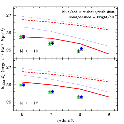
Figure 4: Observed (coloured points) and simulated (curves; from the r24 volume) rest-frame UV luminosity density at z=6–8. We obtain the observed luminosity densities by integrating published luminosity functions down to the indicated limits. The observed luminosity functions are from McLure et al. (2010) (blue) and Bouwens et al. (2009b) (green) at $z=8$; from Ouchi et al. (2009) (green) and McLure et al. (2010) (green) at $z=7$; and from Bouwens et al. (2007) (green) and McLure et al. (2009) (blue) at $z=6$. The two observed densities at each redshift are offset for clarity. Solid and dashed curves indicate the simulated luminosity density including bright galaxies (down to the indicated limits) and all simulated galaxies, respectively, while heavy red and light blue curves include and omit dust reddening, respectively. The simulations and observations are in reasonable agreement at all redshifts although the simulations slightly overproduce the luminosity density at low luminosites and high redshifts, which we ascribe to resolution effects. Broadly, we predict that observations capture less than 20% of the luminosity density at $z\geq 6$.

A key test of galaxy formation models involves the evolution of the star formation rate density. This can be inferred from the UV luminosity density ($\mathcal{L}_{\nu}$), which is simply the integral of the UV LF. In Figure 4, we show the observed (coloured points) and predicted (dark solid curve) rest-frame $\mathcal{L}_{\nu}$ down to $M_{UV}=-19$ (top) and $M_{UV}=-18$ (bottom) at $z=$6–8; see the caption for details. The simulation is in reasonable agreement with observations to $M_{UV}<=-19$ at $z=6$ while it slightly overproduces $\mathcal{L}_{\nu}$ at higher redshifts or when integrating to fainter limits. In both cases, the discrepancies were anticipated by Figure 2, where it is clear that the simulation preferentially overproduces faint ($M_{UV}>-19$) galaxies. As in Figure 2, the observed discrepancies are comparable to the uncertainty that is expected from Poisson errors, cosmic variance, the IMF, and numerical effects.

The question of whether galaxies can contribute enough ionizing photons to reionize the Universe depends sensitively on how much star formation occurs in objects that are fainter than the current observational limit of $M_{1350}<=-18$ (for example, Yan & Windhorst, 2004; Yan et al., 2006). We now estimate this contribution in two ways. First, we directly measure the total predicted $\mathcal{L}_{\nu}$ as a function of redshift within our r24 volume (still including the effects of dust). The dark, lower dashed curve in each panel indicates this total. This curve suggests that current observations do not detect more than $\leq 25$% of the total star formation at $z\geq 6$. In practice, this estimate suffers from numerical resolution uncertainty because the resolution limit of our r24 volume corresponds to a luminosity only slightly fainter than $M_{1350}<=-18$. However, the r12 volume indicates that the true LF continues smoothly to much lower luminosities (Figure 2). Hence we may obtain a second estimate for the total luminosity density as follows: If we assume that the luminosity density per unit halo mass varies slowly with halo mass, then we may compute the unresolved fraction by simply computing the ratio of collapsed matter in halos down to the typical host halo mass at $M_{1350}=-18$ ($5\times 10^{10}M_{\odot}$ at $z=6$ in our simulations) versus the amount of collapsed matter in halos more massive than the photoheating feedback scale of $3\times 10^{8}M_{\odot}$ (Okamoto et al., 2008). Using a standard Press-Schechter calculation, this ratio is 0.079. However, because our outflow model predicts that outflow strength should scale as $M_{h}^{-(1/3)}$, the specific luminosity in low-mass halos is lower, and the unresolved fraction should also be smaller. Correcting for this, we estimate that observations down to $M_{1350}=-18$ probe the brightest 37% of the total luminosity density, in reasonable agreement with our direct numerical estimate.

The lighter solid and dashed curves show how our results change if we neglect dust extinction. Dust extinction suppresses the bright luminosity density by a factor of 2–4 and the total luminosity density by $\sim 50\%$, where the bright galaxies are more extincted because they are more metal-rich and hence more dusty by assumption. The widening gap between the dusty and dust-free luminosity densities from $z=7\rightarrow 6$ tracks a moderate growth in the normalization of the mass-metallicity relation.

We now pause to present our predicted conversion between UV luminosity and star formation rate. For SFHs that are smooth on timescales longer than 10 Myr, this conversion is linear; that is, $\mathrm{SFR}=c_{\mathrm{SFR}}*L_{\mathrm{UV}}$ (Madau et al., 1998; Kennicutt, 1998b). Calculating $c_{\mathrm{SFR}}$ requires knowledge of the galaxy’s SFH, metallicity, and dust extinction. Within our simulations, the SFH and metallicity are predicted self-consistently, hence we may predict $c_{\mathrm{SFR}}$ in the absence of dust. Considering only galaxies with $M_{UV}\leq-18$ and using a narrow boxcar at 1350 Å to compute the UV luminosity, we find that $c_{\mathrm{SFR}}$ is independent of luminosity and equal to $2.0\times 10^{28}$ ergs s^-1 Hz^-1 ($M_{\odot}$ yr^-1)^-1 with a $1\sigma$ scatter of 30% throughout the interval $z=9\rightarrow 6$. This factor assumes the Chabrier (2003) IMF for consistency with our simulations. It may be compared directly with conversions that are used to derive star formation rates from observed UV luminosities at high redshift.

Returning to our predicted star formation histories, Figure 5 compares the simulated and observed stellar mass densities $\rho_{*}$ at $z\geq 6$, again integrating only over galaxies down to $M_{UV}\leq-18$. Comparing the heavy solid red curve with the coloured points reveals that the simulation is in surprisingly good agreement with observations at these epochs. The agreement in the normalizations may be fortuitous. For example, our r12 volume predicts a specific star formation rate 30% lower than the r24 volume in the range where they overlap, which implies that increasing the mass resolution of our r24 volume by a factor of eight would boost the predicted $\rho_{*}$ by roughly this factor. However, the agreement in the evolution of $\rho_{*}$ is nontrivial, and supports the smoothly-rising SFH scenario. To demonstrate this, we use a green dot-dashed curve to illustrate how $\rho_{*}$ would evolve from $z=6\rightarrow 9$ under the hypothesis of constant SFHs. In this trivial case, $\dot{\rho}_{*}(M_{UV}\leq-18)$ is constant and equal to the value at $z=6$. Adopting the observed $\rho_{*}$ and simulated $\dot{\rho}_{*}$ for galaxies with $M_{UV}\leq-18$ (including dust) at $z=6$, we find that the predicted evolution is significantly shallower than observed. The evolution is shallower because, in the realistic case of rising SFHs, galaxies become fainter and drop out of the sample at higher redshifts. This demonstration is “conservative” in two senses: First, our simulations may overproduce $\dot{\rho}_{*}$ at $z=6$ (Figure 2); repeating the exercise with a lower $\dot{\rho}_{*}$ would yield shallower evolution. Second, adopting exponentially-decaying SFHs would lead to increasing $\rho_{*}$ with increasing $z$ (because galaxies near the limit $M_{UV}=-18$ at one epoch would fade below it at later epochs), in serious conflict with observations. Hence the excellent agreement between the predicted and observed slopes is a nontrivial success of the smoothly-rising SFH scenario.

As in the case of the UV luminosity density, we estimate observational incompleteness using our direct numerical predictions. The dashed curve indicates the complete stellar mass density over all galaxies in the simulation. Comparing the heavy solid red and black dashed curves suggests that current observations do not detect more than 20–40% of the true $\rho_{*}$ at $z\geq 6$. This is similar to our estimate of the detected fraction of the UV luminosity density, as expected given that $M_{*}\propto\dot{M}_{*}$.

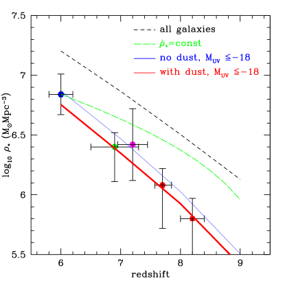
Figure 5: Observed (coloured points) and simulated rest-frame stellar mass density $\rho_{*}$ in our r24 volume at $z=$6–8. The blue hexagon is from Stark et al. (2009); the green hexagon is from Gonzalez et al. (2009); the magenta hexagon is from Labbé et al. (2009); and the red hexagon and square are from Labbé et al. (2009) and (Bouwens et al., 2009b). Observational points have been corrected to account for galaxies brighter than $M_{\mathrm{UV}}\leq-18$ following Labbé et al. (2009), and we have additionally subtracted 0.18 dex to convert to a Chabrier (2003) IMF. Thick red and thin blue solid curves show the simulated $\rho_{*}$ to $M_{UV}<=-18$ including and neglecting dust, respectively, while the dashed curve shows the full simulated $\rho_{*}$. The green dot-dashed curve extrapolates the observed $\rho_{*}$ at $z=6$ backwards assuming constant SFHs and the simulated star formation rate density at $z=6$. The simulated normalization and evolution are in good agreement with observations. Moreover, the predicted evolution is in much better agreement than non-rising SFH scenarios. Current observations probe 20–40% of the total $\rho_{*}$ at $z\geq 6$.

5 Galaxy Colors

5.1 Mean SEDs

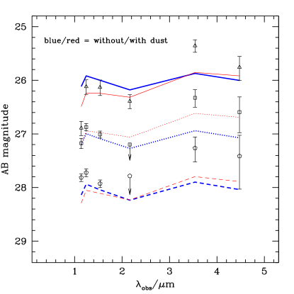
Figure 6: Predicted versus observed mean SEDs at $z=7$ in three bins of $\Delta H=1$ centered on $H_{160}=26,27,28$. Simulated SEDs are plotted with solid, dotted, and dashed curves. Heavy blue and light red curves correspond to simulations without and with dust extinction, respectively. Triangles, squares, and pentagons indicate observations from UV-selected galaxies at $z\sim 7$ (Labbé et al., 2009). Note that the set of model galaxies that falls within each bin depends on whether dust is present. This gives rise to an apparent tendency for the medium and faint bins to be brighter in the dusty models longward of $H_{160}$ owing to their redder SEDs.

In this Section, we study the mean spectral energy distributions (SEDs) of our simulated galaxies in order to gain some intuition into their intrinsic properties and their implied selection function. We begin by showing in Figure 6 the mean SEDs of our simulated galaxies at $z=7$ in three bins of $H_{160}$ (see caption for details). Examining the simulated intrinsic SEDs first (heavy blue curves), we see that both the simulations and the observations indicate SEDs that vary weakly with $H_{160}$, as expected in a scenario where the shape of a galaxy’s SFH varies weakly with its luminosity. All three bins show blue intrinsic UV continua, in good agreement with observations (Bouwens et al., 2009a, b, 2010a; Labbé et al., 2009; Finkelstein et al., 2009). By contrast, the simulated $[3.6\mu]$ fluxes are noticeably weaker than observed at all luminosities. Adding dust extinction reddens the simulated mean SEDs modestly without changing the level of agreement with observations.

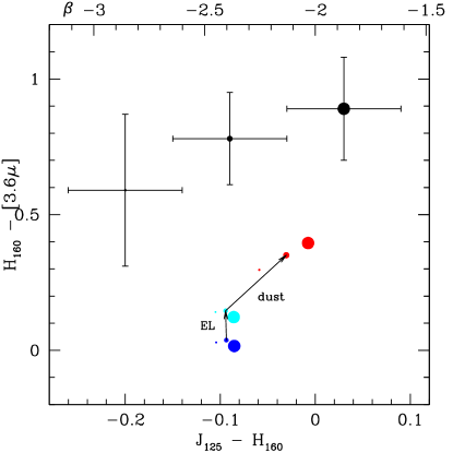
Figure 7: Observed (points with errors) versus simulated (points without errors) colours of galaxies at $z=7$. Circles indicate the mean colours in the same three bins of $H_{160}$ as in Figures 6; circle size scales linearly with $H_{160}$ flux. The effects of emission lines (EL) and dust on the predicted mean colours are shown. The top axis converts $J_{125}-H_{160}$ to UV continuum slope $\beta$ following Bouwens et al. (2010a). The predicted $J_{125}-H_{160}$ colours are quite blue as observed although the faintest bin may be too red, implying that its predicted metallicity is too high. The simulated $H_{160}-[3.6]$ is significantly bluer than observed. Nebular line emission and dust both increase the apparent Balmer break strength, but do not close the gap with observations.

In order to consider the UV continua and apparent Balmer breaks in more detail, we compare in Figure 7 the simulated $J_{125}-H_{160}$ and $H_{160}-[3.6]$ colours. This Figure may be compared with Figure 1 of Labbé et al. (2009). Once dust is included, the simulated UV continua (that is, the $J_{125}-H_{160}$ colours) in the medium and bright bins are consisent with observations owing largely to their young ages (100–150 Myr), low metallicities ($Z/Z_{\odot}<0.5$; Figure 11), and low predicted dust columns.

By contrast, the predicted UV continua in the faintest bin are too red even if dust is omitted. This suggests that their predicted ages or metallicities $Z$ are too high. It is not likely that this discrepancy can be resolved purely through younger ages. This is because the UV continua of Population II stars are too red even in the absence of nebular continuum emission for ages greater than 10 Myr (Bouwens et al., 2010a, Figure 3), and observing populations with ages younger than 10 Myr is unlikely given that these objects have dynamical times of $\sim 100$ Myr. We note that our predicted ages of $\approx 150$ Myr at $z=7$ agree with the recent simulation of Salvaterra et al. (2010), despite incorporating different treatments for both outflows and metal enrichment. A more likely possibility is that $Z$ suffers extra suppression in low-mass galaxies owing to a steeper scaling between the outflow mass loading factor $\eta_{W}$ and the galaxy mass. For example, our simulations currently assume that $\eta_{W}$ varies inversely with the velocity dispersion $\sigma$. Adopting a dependence $\eta_{W}\propto\sigma^{-\alpha}$ with $\alpha>1$ would further suppress $Z$ for faint galaxies because $Z\propto 1./(1+\eta_{W})$ (Finlator & Davé, 2008). Such a model would also bring the faint end of the UV LF into better agreement with observations (Figure 2). A final possibility, as pointed out by Bouwens et al. (2010a), is a small contribution from low-metallicity stars with a top-heavy IMF. Such a population would bluen the UV continuum as long as it did not give rise to significant nebular continuum emission, which in turn would require a high ionizing escape fraction. It would be interesting to explore this possibility within the self-consistent Population III treatment of Salvaterra et al. (2010); unfortunately, these authors did not consider their predicted photometric colours.

Our models qualitatively reproduce the observed tendency for more UV-luminous galaxies to display redder UV continua (Bouwens et al., 2009a, 2010a) owing entirely to the simulated luminosity-metallicity and (assumed) metallicity-reddening relations. Hence the reported colour-magnitude trend could imply a modest trend of increasing dust reddening at higher UV luminosity, as has previously been observed at lower redshifts (Meurer et al., 1999; Shapley et al., 2001). Note, however, that the presence of such a trend in the $z=7$ data remains unclear at present (Schaerer & de Barros, 2010).

Turning to the $H_{160}-[3.6]$ colours, we find that the simulated galaxies generically exhibit significant Balmer breaks at all luminosities, in qualitative agreement with observations. We previously predicted that significant Balmer breaks are expected in Lyman break samples at $z=4$ (Finlator et al., 2006), and Figure 7 now extends this prediction out into the reionization epoch.

In detail, however, the observed breaks are roughly 0.5 mag stronger than predicted. In combination with the blue UV continua, these colours pose a challenge for our simulations. This result is similar to the finding by Labbé et al. (2009) that linearly rising SFHs do not produce Balmer breaks stronger than $H_{160}-[3.6]=0.3$ mag whereas the observations require break strengths of 0.5 mag or stronger. One possible explanation is nebular line emission. For example, Schaerer & de Barros (2009, 2010) have used stellar population synthesis models including treatments for nebular continuum and line emission to show that the strong apparent Balmer breaks observed at $z\geq 6$ can be mimicked by nebular line emission from extremely young ($<10$ Myr), low-metallicity populations (see also Zackrisson et al., 2008; Ono et al., 2010). Our simulations provide physically-motivated priors for the typical ages and metallicities at these epochs, allowing us to predict the strength of the nebular emission lines. We find that line emission improves the agreement with the observed $H_{160}-[3.6]$ colour by $0.1$ mag. We do not find that line emission can completely explain the observed $H_{160}-[3.6]$ colours because our relatively evolved, enriched stellar populations do not yield sufficiently strong emission line equivalent widths (in contrast to the wide range of models explored by Schaerer & de Barros 2009). Note that this conclusion is conservative in the sense that, in modeling emission lines, we have assumed an ionizing escape fraction of zero. For sufficiently large ionizing escape fractions that observed galaxies could contribute significantly to reionization (10–50%), the lines would be correspondingly weaker.

Another possible explanation for the observed colours is inherently bursty SFHs. For example, Labbé et al. (2009) show that only highly bursty SFHs can simultaneously reproduce the observed $J_{125}-H_{160}$ and $H_{160}-[3.6]$ colours at low masses (and then only barely). Encouragingly, they also find that such a model would not overproduce the scatter in the observed SFR-$M_{*}$ relation. Hence it is possible that boosting our mass resolution would resolve more minor perturbations and instabilities, giving rise to more bursty SFHs and redder predicted $H_{160}-[3.6]$ colours. We can explore this possibility by appealing to the tendency for $H_{160}-[3.6]$ to vary weakly with luminosity (Figure 6) and examining the trend at lower masses in our higher-resolution volume. We find that increasing our mass resolution by a factor of eight boosts $H_{160}-[3.6]$ by 0.02 mag on average. This is quite small compared to the 0.5 mag discrepancy with observations, hence if resolution limitations are to blame then overcoming them may require “zoom-in” simulations of overdense regions given that our current simulations already probe the limits of what is computationally feasible.

It is also possible that the discrepancy owes to a patchy dust scenario in which a fraction of the lines of sight through an LBG’s interstellar medium (ISM) are optically thick to UV; this would suppress the rest-frame UV much more strongly than the optical. However, it is difficult to reconcile this scenario with the blue observed UV continua, which seem to imply that these galaxies are essentially dust-free.

Is it possible that a different treatment for galactic outflows could suppress the simulated SSFR, thereby deepening the predicted Balmer breaks? As can be seen from Figure 2 of Davé (2008), the predicted SSFR is relatively insensitive to the details of the outflow treatment. This is because changing the outflow strength broadly increases or decreases $M_{*}$ and SFR together, without substantially changing their ratio (see also Dutton et al., 2009; Bouché et al., 2009). Hence it is unlikely that the predicted $H_{160}-[3.6]$ colours could be made redder by modifying our outflow treatment.

Finally, it cannot be ruled out that the photometric uncertainties reported by Labbé et al. (2009) underestimate the true errors because the stacked fluxes could be biased by the presence of bright outliers. For example, if (despite their careful analysis) the rest-frame optical flux of a fraction of the sources in each bin were contaminated by incompletely-subtracted neighboring objects, the resulting error in the stacked SED would be difficult to detect given the small number of sources in each bin. This reinforces the need for larger samples both in order to reduce errors and in order to allow for more accurate uncertainty estimates.

In summary, our simulations produce blue UV continua and significant Balmer breaks at all luminosities, in qualitative agreement with observations. The faintest observed galaxies are 0.1 mag bluer than predicted, which may suggest that our feedback model insufficiently suppresses the metallicities of low-mass galaxies. Our predicted UV continua qualitatively reproduce the reported colour-magnitude trend as long as we include our metallicity-dependent dust reddening prescription. The simulations produce apparent Balmer breaks that are weaker than observed, even if we correct for resolution effects and account for nebular line emission. This is the most dramatic discrepancy that we have found, and it emphasizes the need for a better observational understanding of the nature of the observed apparent Balmer breaks at $z\geq 6$ through $K$-band imaging, mid-infrared spectroscopy, or mid-infrared imaging with improved spatial resolution.

5.2 Direct Spectral Energy Distribution Fitting

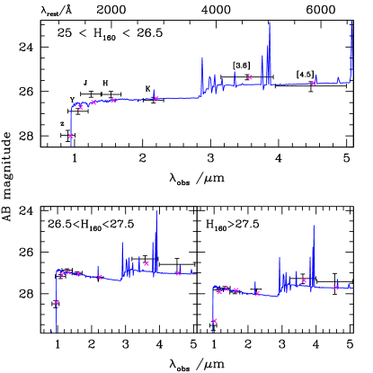
Figure 8: Black points with errors denote the stacked SEDs of $z\sim 7$ LBGs from Labbé et al. (2009); the $H_{160}$ magnitude ranges for each bin are indicated. The blue curve indicates the spectrum of the best-fit numerically-simulated galaxy. Magenta crosses indicate synthetic photometry of that spectrum, offset slightly in wavelength for clarity. The simulated spectra yield reasonable agreement at all wavelengths, although the WFC3/IR measurements in the brightest bin are not well-fit. Optical emission lines readily explain the observed $[3.6]-[4.5]$ colours.

In Section 5.1, we compared the predicted and observed colours of galaxies at $z\sim 7$ without allowing the redshift or the amount of dust extinction to vary. This approach is justified if the photometric redshifts are accurate and the dust extinction is negligible. On the other hand, given that we do not model the dust extinction self-consistently and that the redshift is not well-constrained, a complementary approach is to allow these parameters to vary freely and ask how well the simulations can account for observations in principle. In this Section, we use our Bayesian SED-fitter spoc (Finlator et al., 2007) to determine how well the smoothly-rising SFHs fit observed SEDs at $z\sim 7$ and discuss the implied physical properties.

Here we briefly review spoc; for details and tests see Finlator et al. (2007). spoc operates similarly to other SED-fitters. Starting with a set of model SFHs, it generates a library of SEDs by resampling the SFHs over a grid of redshift $z$ and dust column $A_{V}$. Note that, in an improvement over our previous work, we include optical emission lines as described in Section 2.2. After comparing the library SEDs with the measurements, it uses a Bayesian analysis to derive the posterior probability for the various physical parameters from the likelihoods ($\exp(-\chi^{2}/2)$) and any priors. The novelty of this approach is that we directly adopt numerically simulated SFHs and metallicities rather than assuming toy-model SFHs (for example, constant or declining). This imposes physically-motivated priors on the results because the prior probability of a given combination of age, metallicity, $M_{*}$, and SFR is proportional to the number of model galaxies that form with these parameters. It is for this reason that, in contrast to conventional SED-fitting studies, spoc only resamples the model SFHs in $z$ and $A_{V}$. The number of free parameters is difficult to define given that the simulations do not sample parameter space uniformly. However, given that metallicity and SFR correlate tightly with $M_{*}$ whereas age varies only with redshift, there are effectively only three, namely $M_{*}$, $z$, and $A_{V}$. The resulting likelihoods are equally as interesting as the constraints because they quantify how well numerical SFHs can account for the full SEDs of individual objects, automatically identifying observed colours that challenge the models.

As a test of how well our numerical simulations can account for the full SEDs of reionization-epoch galaxies, we apply spoc to the three binned SEDs at $z\sim 7$ from Labbé et al. (2009) in order to take advantage of their high signal-to-noise. We derive our model SFHs from snapshots of our 24 $h^{-1}{\rm Mpc}$ volume at a number of discrete redshifts between $z=6$–8. We do not consider low-redshift solutions (see McLure et al., 2009). Perturbing each model galaxy in redshift and sampling 100 different values of $A_{V}$ between 0–1.5, we generate a library of 5 million model SEDs for comparison. We treat detections with less than $2\sigma$ significance as $2\sigma$ upper limits and adopt the reported measurements and errors in the other bands. We adopt the WFC3/IR $Y_{105}$ and VLT/ISAAC $K_{s}$ bands to compute simulated $Y$ and $K$ fluxes, respectively.

In Figure 8, we compare the observations (black points) with the spectrum of the best-fit combination of model SFH, redshift, and $A_{V}$ (blue curve) and its associated photometry (magenta crosses). Examining the brightest bin first (top panel), we find that our best-fit SED matches the observed fluxes in all bands other than $J_{125}$ and $H_{160}$, both of which it underproduces by $\approx 2\sigma$. Intriguingly, we find that optical emission lines completely explain the observed $K-[3.6]$ and $[3.6]-[4.5]$ colours. Many reionization-epoch SEDs show evidence for a blue optical continuum suggestive of optical emission lines (Labbé et al., 2009; Gonzalez et al., 2009). Our modeling suggests that these colours are real rather than reflecting observational uncertainty (for example, in the IRAC measurements), with several implications. First, it reinforces the need for SED-fitting studies to account for nebular emission (Schaerer & de Barros, 2009, 2010). Second, it surprisingly suggests that the difficulty with the observed $H_{160}-[3.6]$ colours (Figure 7), if observational in origin, may owe as much to the WFC3/IR as to the IRAC bands given that the $K-[3.6]$ and $[3.6]-[4.5]$ colours are not difficult to reproduce. Finally, it reinforces the need for deep $K$-band imaging in order to constrain the strength of the Balmer Break.

We may derive constraints from our posterior probability distributions by marginalizing over all but one parameter at a time and determining the resulting 68% confidence intervals. This method generally suffers from significant degeneracies between the derived age, metallicity, and dust extinction (for example, Shapley et al., 2001; Papovich et al., 2001). However, restricting our attention to the SFHs that arise within our simulations partially breaks these degeneracies because the predicted range of SFHs is narrow, effectively introducing tight priors (for details, see Finlator et al. 2007). We find $z=6.7\pm 0.1$, $A_{V}=0.6\pm 0.1$, $\log(M_{*}/M_{\odot})=9.6\pm 0.1$, $\dot{M}_{*}=16.0\pm 3.8M_{\odot}\mbox{yr}^{-1}$, and $Z=0.007\pm 0.0009$. The inferred SFR is 60% larger than inferred by Labbé et al. (2009), and the inferred stellar mass is 10% lower (both numbers are corrected for the different assumed IMFs). Meanwhile, the inferred dust column is much larger than would be expected from the blue $J_{125}-H_{160}$ colour. This explains why the model SED is too red in $H_{160}-[3.6]$ whereas, with our fiducial dust prescription, it was too blue (Figure 7). Not surprisingly, the associated $J_{125}-H_{160}$ colour is now also too red whereas it was in good agreement with the observed colour in Figure 7. These constraints are driven largely by the $K$–$[4.5]$ bands, and the lower stellar mass is permitted in part by the inclusion of nebular emission lines (for example, Schaerer & de Barros, 2010; Ono et al., 2010).

In the bottom panels, we compare the stacked SEDs from the medium and faint bins of Labbé et al. (2009) with the best-fit model SEDs. These bins yield generally better fits to our models than the brighter bin. As before, the simulated SEDs readily reproduce the observed $[3.6]-[4.5]$ colours owing to the presence of optical emission lines. The medium stack implies the physical parameters $z=6.8\pm 0.1$, $A_{V}=0.08\pm 0.08$, $\log(M_{*}/M_{\odot})=8.8\pm 0.1$, SFR=$3.1\pm 0.4M_{\odot}\mbox{yr}^{-1}$, and $Z=0.0040\pm 0.0006$, while the faint stack corresponds to $z=6.9\pm 0.1$, $A_{V}=0.09\pm 0.08$, $\log(M_{*}/M_{\odot})=8.5\pm 0.1$, $\dot{M}_{*}=1.5\pm 0.3M_{\odot}\mbox{yr}^{-1}$, and $Z=0.0032\pm 0.0007$. As before, the stellar masses are lower than would be inferred without emission lines. Meanwhile, the inferred SFRs are 10–30% lower than inferred by Labbé et al. (2009) (after accounting for the different IMFs) owing to the low predicted metallicities. The inferred dust columns are significantly lower than in the bright bin. Note, however, that deeper observations in $K$ may eventually demand higher dust columns in the faint bins as well.

5.3 Survey Completeness

We may use our simulated SEDs to predict the completeness of current surveys. In detail, of course, completeness varies with the selection strategy. However, a tight correlation between stellar mass and SFR implies that the completeness of UV-selected samples is dominated by the detection limit rather than by colour cuts (Finlator et al., 2006). This is especially true when the dust column is low. For example, the colour cuts in Oesch et al. (2010a) do not eliminate any of our simulated galaxies at $z=7$.

In Figure 9, we plot using heavy curves the number fraction of galaxies that are selected by the $5\sigma$ detection limits in $J_{125}$ and $H_{160}$ of Bouwens et al. (2010a) versus stellar mass both with and without dust. Galaxies with $M_{*}\geq 10^{9}M_{\odot}$ are selected efficiently assuming that dust reddening is small ($E(B-V)\leq 0.05$) owing to their high star formation rates. Dust increases the 50% completeness limit from $10^{8.7}M_{\odot}$ to $10^{8.9}M_{\odot}$ by extincting galaxies whose UV luminosities are already near the detection limits. Galaxies with stellar masses less than $10^{8.5}M_{\odot}$ are not selected efficiently regardless of dust because their star formation rates are too low. The $5\sigma$ detection limit for a $10^{4}$ second exposure through the JWST/NIRCAM F200W filter will be $K=29.72$; we show how this improves the mass completeness using light curves. Clearly, a relatively shallow JWST exposure will readily detect objects that are 10% as massive as the least massive objects detected in the WFC3/IR ERS fields. The impact of dust extinction will be weak owing to the low metallicity (Figure 11).

These results are robust to our choice of input physics or mass resolution. This is because the mass completeness is mostly sensitive to the specific star formation rate, which in turn is relatively insensitive both to our choice of outflow strength and mass resolution.

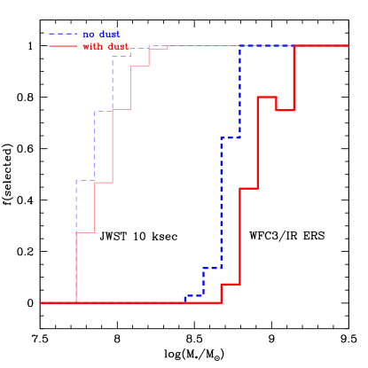
Figure 9: Completeness versus stellar mass at $z=7$. Curves show how the number fraction of galaxies that are selected by two different criteria varies with stellar mass in simulated catalogs with (solid red) and without (dashed blue) dust reddening. Heavy curves correspond to the current $5\sigma$ limiting magnitude in the WFC3/IR ERS fields of $J\leq 27.7\wedge H\leq 27.4$ (Bouwens et al., 2010a). Light curves correspond to the $5\sigma$ detection limit for a 10,000 second exposure in the JWST/NIRCAM F200W band. Current surveys detect most galaxies more massive than $10^{9}M_{\odot}$ and few that are below $10^{8.5}M_{\odot}$, while JWST will easily detect objects that are 10% as massive.

6 Physical Properties

In this section, we summarize the predicted physical properties of our simulated galaxies at $z\geq 6$, where possible comparing with observational inferences. The most important physical process impacting these predictions is our simulation’s implementation of momentum-drive outflows, and we have previously explored the effects at $z=6$ of varying our outflow treatment in DFO06.

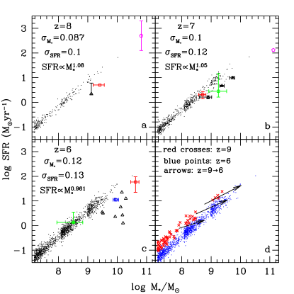
Figure 10: Panels a–c show simulated (black points) and observed (coloured shapes) SFR-$M_{*}$ relationships. The three simulated loci correspond to our three volumes, and their good agreement suggests that numerical errors are weak. We include the slope and dispersion about the best-fit linear relation from the r24 volume at each redshift. Panel d shows the simulated relationships at $z=9$ (red crosses) and $z=6$ (blue points) as well as typical evolution of individual galaxies from $z=9\rightarrow 6$ (arrows). The red square at $z=8$ is from Bradley et al. (2008), where we assume constant star formation and $Z_{*}=0.0004$; the black triangle corresponds to the best-fit SFH to the $z=7.7$ stack of Labbé et al. (2009); and the magenta hexagon is Object 1 from Capak et al. (2009). At $z=7$, black triangles are the stacked results from Labbé et al. (2009); the red square is from Egami et al. (2005), where the point represents the average of the inferences assuming a 100 Myr exponentially decaying SFH over the different assumed metallicities, and the errors reflect this error added in quadrature to assumed photometric errors of (5%, 20%) in the (SFR, mass); the magenta hexagon is Object 3 from Capak et al. (2009); and the green square is the $z=6.6$ LAE stack of Ono et al. (2010), where we plot result from the “pure stellar” model with $Z/Z_{\odot}=0.2$. At $z=6$, the blue pentagon is LA34 from Lai et al. (2007); the red square is from Dow-Hygelund et al. (2005); the black triangles are from Eyles et al. (2007); and the green square is from the stacked SED at $z=5.7$ of Ono et al. (2010) assuming “pure stellar” models with $Z/Z_{\odot}=0.2$. We have subtracted 0.18 dex from all observationally inferred SFR and $M_{*}$ to adjust from the Salpeter to the Chabrier IMF. Our simulations predict that SFR $\propto M_{*}$, with tight scatter and a weakly-evolving normalization. The slope and evolution of the simulated trend are in good agreement with observations, but the normalization may be offset by a factor of 2–3.

6.1 Star Formation Rates

We show in Figure 10 how SFR relates to $M_{*}$ in our simulated catalogs (black points) at four different redshifts. Broadly, we predict SFR$\propto M_{*}^{\mbox{0.95--1.05}}$ at all redshifts, confirming our previous results (DFO06). The predicted slope at $z=7$ of 1.05 is in excellent agreement with the reported slope of $1.06\pm 0.1$ (Labbé et al., 2009), and the agreement is good at the other epochs as well. This comparison is a nontrivial test of our model, and given that our simulations were not tuned to reproduce such a trend—in fact, this class of simulations predicted it (Davé et al., 2000; Weinberg et al., 2002)—the level of agreement is remarkable.

There are two possible interpretations for a near-unity slope. One possibility is that galaxies begin forming stars at different epochs, but once they begin, their growth is exponential with a timescale $M_{*}/\dot{M}_{*}$. This timescale is observed to be $\approx 500$ Myr at $z=6$ (Stark et al., 2009), although our simulations indicate somewhat shorter timescales of 200–350 Myr (note that accounting for optical emission lines will bring observations into closer agreement with our predictions; Section 5.2). The short growth timescales could then imply a bursty star formation scenario in which galaxies “turn on” at different times, form stars with a short duty cycle and a constant exponential growth timescale, and then fade into a quiescent state (Stark et al., 2009). There are two difficulties with this picture. One is that it is not obvious why galaxies that begin forming at very different times should nonetheless obey the same exponential growth timescale with negligible scatter. The other is that bursty models predict a large population of quiescent galaxies at $z\geq 4$ that has not been observed (Brammer & van Dokkum, 2007). We will return to these points in Section 7.

A second interpretation of the near-unity slope is that SFHs at $z\geq 6$ have a scale-invariant shape. This is because, if all galaxies begin forming stars at the same time and with the same SFH shape, then the SFR and the $M_{*}$ both vary linearly with an overall scale factor. Consequently, the slope remains near unity until a mass-dependent process such as hot-mode accretion or AGN feedback breaks the scale-invariance and flattens the slope (Davé, 2008). In this smoothly-rising SFH scenario, the growth timescale is dominated by smooth inflows, which in turn are regulated by the competition between the growth of halo potential wells and the decrease in the cosmic density (Bouché et al., 2009; Dutton et al., 2009). It is not easy to distinguish observationally between the bursty and the smoothly-rising scenarios using UV-selected samples, although our models (and, for that matter, all hydrodynamical simulations) support the latter view. However, we will discuss other observational probes in Section 7.

The predicted normalization may be slightly offset from observations. This offset could have two possible implications. First, it suggests that observationally inferred stellar masses are too high because they do not include the effect of optical emission lines. Accounting for this would likely reduce observationally inferred stellar masses by 0.1–0.3 dex (Figures 7 and 8), improving the agreement with predictions. In support of this view, Labbé et al. (2009) have found that applying an observationally-motivated estimate for the strength of the OII emission line lowers the typical inferred $M_{*}$ at $z=7$ by 0.17 dex. The second implication is that our simulated SFRs are slightly too high, which we previously noticed evidence for in Figure 2. It is tempting to suppose that strengthening our outflows would solve this problem. Unfortunately, as noted in Section 5, this would not suppress the predicted SSFR because increasing the outflow mass-loading factors reduces $M_{*}$ and $\dot{M}_{*}$ together without changing their ratio (see also Dutton et al., 2009). Hence it is not simple to understand how the bulk of the offset could be attributed to our input physics.

The predicted dispersion about the mean trend is $\approx 0.1$ dex at all redshifts. This tight scatter reflects the tendency for star formation to be driven by smooth gas accretion rather than by interactions (Kereš et al., 2005; Birnboim et al., 2007). It is somewhat less than the reported scatter of 0.25–0.3 dex at $z\sim 7$ (Labbé et al., 2009). Given that observational uncertainties boost the observed scatter, it is possible that the true scatter is consistent with our predictions. It is also possible that our limited numerical resolution does not account fully for the minor interactions or discrete infalling clouds that perturb galaxies away from their equilibrium SFR. We evaluate this possibility by plotting the predicted SFR-$M_{*}$ trend from all three of our simulation volumes at each redshift (hence the three separate “clumps” in the simulated locus). These three volumes span a factor of 64 in mass resolution and should immediately reveal which predictions are strongly sensitive to numerical effects. The offsets in the trends are small compared to the scatter, and the scatter does not vary with resolution. This indicates that the predicted trends are numerically converged. Moreover, it is interesting to note that the mass resolution of our $12h^{-1}{\rm Mpc}$ simulation is 50% higher than the gas-phase mass resolution with which Mihos & Hernquist (1996) demonstrated that mergers can boost SFRs of MW-scale galaxies by factors of 10–100. The fact that our predicted SFR-$M_{*}$ scatter remains small despite our resolving power supports the view that the predicted scatter is robust to resolution limitations, and that dramatic merger-driven starbursts are indeed uncommon at high redshift.

Dutton et al. (2009) use a semi-analytic model for the growth of disk galaxies within a smoothly-accreting halo to predict a scatter of $\sim 0.1$ dex at all redshifts. They attribute this to scatter in the mass accretion histories of the host halos. They then speculate that the larger observed scatter could owe to scatter in the gas accretion rate at fixed halo mass, which their model does not account for. Our simulations account for this effect self-consistently, hence the fact that our predicted scatter agrees with theirs argues that the observed scatter is not dominated by scatter in the gas accretion rate at fixed halo mass.

In the bottom-right panel, we show how galaxies’ masses and SFRs evolve from $z=9\rightarrow 6$ in each of our simulation volumes. Red crosses and blue points show the simulated loci at $z=9$ and 6, respectively. Comparing these loci reveals that the SFR at a given $M_{*}$ (that is, the normalization of the $M_{*}$-$\dot{M}_{*}$ relation) is predicted to decline by $\approx 0.3$ dex from $z=9\rightarrow 6$. As we have already seen, observations also indicate that this normalization evolves weakly out to at least $z=8$, qualitatively supporting this picture (Gonzalez et al., 2009; Stark et al., 2009). This slow evolution indicates that galaxies grow roughly exponentially during this epoch, as can also be seen from the shallow evolution of the slope of the mean SFH after $z=9$ in Figure 1. As pointed out by Stark et al. (2009), the only smooth SFH that is consistent with these trends is a rising one.

In order to illustrate how this works, we have added arrows indicating the typical evolution of individual galaxies during this epoch. We trace this evolution by looping through the 10 most massive galaxies identified in each simulation at $z=6$ and searching for their most massive progenitors at $z=7$–9. We then average the masses and SFRs of these 10 galaxies at $z=6$ and their most massive progenitors at $z=9$; the resulting average evolution is representative of how all galaxies are predicted to evolve. Galaxies evolve in a direction that is slightly shallower than the mean trend at a given redshift. The tendency to evolve nearly parallel to the observed trend indicates smoothly-rising, nearly exponential growth while the slightly shallower slope reflects a slow decline in gas accretion rates owing to cosmological expansion (Bouché et al., 2009).

Observational inferences suffer from two systematic biases, either of which could introduce artificial offsets or scatter at each redshift. First, the relevant data were measured by many different groups (see the caption), each of which introduces slightly different photometric techniques and selection biases. The reported errors may be underestimated (Schaerer & de Barros, 2010) although side-by-side comparisons suggest that this problem is not large (Finkelstein et al., 2009). Second, different groups used different assumptions in SED-fitting. This introduces scatter because the choice of SFH and stellar metallicity biases the inferred stellar mass by 10–30% on average, with biases of up to a factor of 10 possible for certain model SFHs (for example, Shapley et al., 2001; Papovich et al., 2001; Finlator et al., 2007; Maraston et al., 2010). It would be of interest to reproduce these observational constraints using unified modeling assumptions at all epochs in order to minimize these effects (for example, Schaerer & de Barros, 2010). Viewed differently, however, it is intriguing that, despite the variety of observational and modeling techniques that underlie these observations, the resulting constraints tell a consistent story: The observed SFR-$M_{*}$ trend obeys a near-unity slope, its normalization evolves slowly, and it may be slightly offset to lower SFR or higher $M_{*}$ than predicted by our model. It is not unreasonable to suppose that applying a consistent set of modeling assumptions to these data would only tighten and reinforce the inferred trends.

In summary, current observations indicate that our simulations reproduce the observed slope and evolution of the SFR-$M_{*}$ trend at $z\geq 6$, while the normalization may be somewhat offset and the scatter is 50% lower than observed. The near-unity slope supports the view that observed reionization-epoch galaxies began forming stars at similar epochs and possess SFHs that differ from one another only by a scale factor. The offset in the normalization, if confirmed, indicates that the inferred stellar masses are too high because they do not correct for optical emission lines. The weak observed evolution in the normalization is inconsistent with any smooth SFH other than a rising one. The small predicted and observed scatters are broadly consistent with the view that high-redshift star formation is driven predominantly by gas inflows rather than mergers, while the fact that the observed scatter is larger may reflect observational uncertainties.

6.2 Metallicities

Direct observations of gas-phase abundances now indicate that galaxies exhibit progressively lower metallicities at higher redshifts (Erb et al., 2006; Maiolino et al., 2008). In DFO06, we showed that this occurs naturally in the hierarchical growth scenario and predicted that observable galaxies at $z\sim 6$ should exhibit metallicities less than one tenth solar. Since then, a number of works have lent qualitative support to this prediction by noting that subsolar metallicities yield better fits to observed SEDs at $z\geq 6$ than solar metallicities (for example, Eyles et al., 2007; Stark et al., 2009; Bouwens et al., 2010a; Labbé et al., 2010).

On the other hand, an important result from DFO06 was the prediction that very little of the observable star formation at $z\sim 6$ should result in primordial-metallicity “Population III” stars because metal enrichment occurs so quickly. Given that our updated simulations incorporate significantly more realistic treatments for metal enrichment (Section 2), it is of interest to determine whether these results have changed. To this end, we use this section to update our predicted mass-metallicity relation at $z\geq 6$ and show that improving our treatments for metal enrichment revises our predicted metallicities up rather than down, supporting our view that reionization-epoch galaxies should not exhibit a significant contribution from Population III stars.

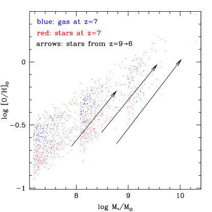
Figure 11: Simulated SFR-weighted gas metallicity (blue top locus) and mass-weighted mean stellar metallicity (red bottom locus) versus stellar mass at $z=7$. We assume a solar photospheric oxygen mass fraction of 0.00574 (Asplund et al., 2009). The three “clumps” indicate our three simulation volumes. The arrows indicate the mean evolution in stellar mass and stellar metallicity of the 10 most massive galaxies in each simulation volume from $z=9\rightarrow 6$. Observable galaxies are already enriched above $0.1Z_{\odot}$ by $z=7$. Their evolution is slightly steeper than the mean trend at a given epoch owing to weak evolution in the normalization of the mass-metallicity relation.

In Figure 11, we show with red points (bottom locus) the mass-weighted mean stellar oxygen metallicities of our simulated galaxies at $z=7$, normalized to the solar photospheric oxygen mass fraction. Broadly, we predict that observed reionization-epoch galaxies possess metallicities greater than $0.1Z_{\odot}$. We also predict a tight trend with $\approx 0.1$ dex of scatter in the residuals, similar to our previous finding at $z=2$ (Finlator & Davé, 2008). Note that the predicted relation for the iron mass fraction is similar but shifted down by 0.2 dex, reflecting the weak contribution of prompt Type Ia supernovae at early times.

The upper, blue locus shows the SFR-weighted mean gas-phase oxygen metallicities for the same galaxies. These points predict that gas metallicities follow the same trends as the stellar metallicities but boosted by $\approx 0.2$ dex becase stellar metallicities reflect the lower metallicities that characterized each galaxy’s progenitors. This figure may be compared to Figure 5 of DFO06, where we used a similar set of simulations to predict that the gas-phase metallicities at $z=$6–8 were generally larger than 1/30$Z_{\odot}$. Our current simulations track metal enrichment significantly more realistically, as summarized in Section 2. Given this abundant increase in realism, the fact that our newer simulations predict higher metallicities than our previous work underscores the conclusion that observable stellar populations at $z=$6–9 should not contain a significant stellar mass fraction below the Population III threshold of $[O/H]<-3$ (Bromm & Larson, 2004).

We use arrows to indicate how galaxies evolve in stellar mass and stellar metallicity from $z=9\rightarrow 6$ in each of our three simulation volumes (the gas-phase metallicity is similar, but shifted up by 0.2 dex). We compute this mean evolution using the 10 most massive galaxies in each volume at $z=6$ as described in Section 6.1. Galaxies evolve along a direction that is slightly steeper than the mean trend at $z=7$. This can be understood as follows (see also Finlator & Davé, 2008): In the presence of strong outflows, galaxy metallicities closely track the equilibrium metallicity $Z=y/(1+\eta_{W})$, where $y$ is the metal yield and $\eta_{W}$ is the mass-loading factor, or the rate at which material enters the outflow divided by the SFR. This equilibrium metallicity owes to strong coupling between the inflow, star formation, and outflow rates. In the momentum-driven wind scenario, $\eta_{W}$ shrinks with increasing mass, hence the equilibrium metallicity grows with increasing mass. The tendency for galaxies to evolve slightly more steeply than the mean trend at a given epoch reflects the prediction that the normalization of the mass-metallicity relation grows by 0.2 dex from $z=9\rightarrow 6$.

To understand the increase in our predicted metallicities with respect to DFO06, note that, at a fiducial stellar mass of $10^{9}M_{\odot}$ and redshift $z=6$, DFO06 predicted a gas-phase metal mass fraction of 0.002, whereas our current simulations predict a mass fraction of 0.006 overall, with 0.005 of this in oxygen alone. This increase owes to the various improvements within both our simulations and our analysis: The newer code predicts noticeable $\alpha$ enhancements at $z=6$; the adopted mass-loading factors were twice as large at a given halo mass in our previous simulations; and our adoption of a Chabrier (2003) IMF when computing the yields significantly boosts the enrichment rates. Each of these effects boosts the predicted gas-phase metallicities by 0.1–0.3 dex, hence an overall factor of three increase is not surprising. This difference may be regarded as an estimate in the uncertainty owing to our imperfect understanding of how metals are created and transported (although we believe that our current simulations are the more realistic). For example, if we were to re-run our simulations with higher mass loading factors in order to improve the agreement between the simulated and observed UV LFs (Figure 2), our predicted metallicities would shrink by 0.1–0.3 dex. Broadly, however, this uncertainty is far too small to change the fundamental conclusion from Figure 5 of DFO06: Observable stellar populations at $z=$6–9 are robustly predicted to have metallicities that are well in excess of 0.01$Z_{\odot}$, hence it should be possible to understand their SEDs without reference to the predicted SEDs of Population III stars.

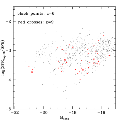
Figure 12: The fraction of star formation occurring in gas with oxygen mass fraction less than $10^{-3}Z_{\odot}$ as a function of absolute magnitude at $z=9$ (red crosses) and $z=6$ (black points). A residual fraction of Population III star formation is predicted to persist even in bright galaxies at $z=6$.

Despite the fact that star formation at $z\geq 6$ is dominated by metal-enriched gas, a residual fraction of metal-poor star formation is predicted to persist even in observable galaxies. To estimate this, we have computed for each simulated galaxy the fraction of star formation occurring in gas whose oxygen mass fraction falls below $10^{-3}Z_{\odot}$. In Figure 12, we show how this fraction varies with absolute magnitude at $z=6$ (points) and $z=9$ (red crosses). At both redshifts, we predict that roughly $10^{-3}$ of all star formation occurs in metal-poor gas, fairly independent of luminosity. Hence it is entirely possible that the observed reionization-epoch samples contain a tiny fraction of Population III star formation although the impact on the total SEDs is negligible. In detail, comparison of the three simulated loci suggests that our simulations do not completely resolve the metal-mixing processes that determine the Population III fraction. Extrapolating the trend from the highest-resolution simulation, we find that galaxies with $M_{UV}=-17$ may have a Population III fraction as high as 1%. This population may eventually be detectable through its enhanced rate of pair production SNe or GRBs. Note that these results are in qualitative agreement with previous suggestions that a residual level of Population III star formation persists after $z=6$ (Tornatore et al., 2007; Johnson, 2010; Maio et al., 2010; Trenti et al., 2009).

Salvaterra et al. (2010) have recently used observed samples at $z=5$–10 to test the predictions of a cosmological hydrodynamic simulation that differs from ours in three major respects: First, they incorporate an explicit treatment for the transition from Population III to Population II star formation whereas our simulations do not treat Population III. Second, they treat the formation, destruction, and dispersal of dust grains in detail in order to predict the dust reddening whereas our model ties the normalization of a foreground dust screen to local observations. Finally, their simulations model galactic outflows under the assumption that the mass-loading factor and wind speeds do not vary (Springel & Hernquist, 2003) while our simulations assume momentum-driven winds (Murray et al., 2005). Despite these differences, their finding that the impact of Population III stars on observable $z=6$–8 galaxies is slight ($\leq 1\%$ of the UV luminosity for $M_{UV}<-18$) is qualitatively consistent with our own results, and justifies our decision to neglect the associated processes in our simulations.

7 Interpreting the Observed Halo Occupancy

Figure 13: top The simulated LBG HOD at $z=5.5$ for samples brighter than $M_{1350}\leq-18$ (solid blue) and -19 (dashed red). The arrows indicate the hypothetical minimum halo mass for each sample (see text). The simulated HOD lies well below unity for low-mass halos $\log(M_{h}/M_{\odot})<11$ owing to strong outflows, and it climbs gradually owing to significant scatter in the relationship between halo mass and $M_{1350}$. bottom The cumulative occupancy for samples satisfying the same luminosity cuts as in the top panel. Thick and thin curves show the cumulative halo occupancy with and without additional galaxies in halos that host more than one galaxy satisfying the luminosity cut. The predicted occupancies lie within the observationally inferred range of 0.15–0.6 (Lee et al., 2009), but they reflect a suppressed HOD owing to outflows rather than a star formation duty cycle.

Up until this point, we have used a variety of arguments to demonstrate that, if Lyman Break galaxy (LBG) SFHs are smooth, then observations indicate that they must be rising rather than constant or declining. We have not yet considered the possibility that LBG SFHs are highly bursty. For example, Lee et al. (2009) recently used accurate clustering observations at $z=4$–6 to show that the fraction of massive halos that host LBGs (hereafter, the “occupancy”) is likely less than unity, and interpreted this as evidence that LBGs have short star formation duty cycles. Subsequently, Stark et al. (2009) built upon this idea to speculate that the progenitors of LBGs observed at one epoch may not be observable at earlier epochs since the progenitors’ SSFRs would violate the observed non-evolving SSFR. This interpretation echoes Ferguson et al. (2002), who used rest-frame UV-optical measurements combined with toy-model SFHs to demonstrate that the progenitors of LBGs at $z=3$ cannot dominate the observed star formation rate density at $z=4$ if SFHs are smooth. In this Section, we explore how our simulations populate dark matter halos with LBGs and argue that outflows naturally give rise to the observed occupancy, with the implication that there is no conflict between clustering observations and the smoothly-rising SFH scenario. We defer a more direct comparison of our predicted clustering properties with observations to future work.

7.1 Halo Occupation Distribution

For reference, we begin by reviewing how an observed sample’s occupancy may be inferred from its LF and clustering behavior. The connection is made by modeling the underlying galaxy population’s halo occupation distribution (HOD; Berlind & Weinberg 2002; Bullock et al. 2002), or the mean number of observable galaxies as a function of halo mass. This in turn derives from the survey selection probability, the LF of isolated halos, and the subhalo mass function (Yang et al., 2003; Lee et al., 2009). To be explicit, let us define the isolated halo LF $dN_{g}/dL(M)$ as the intrinsic number of galaxies with luminosity between $L$ and $L+dL$ in a halo of mass $M$; the selection probability for galaxies of luminosity $L$ as $p(L)$; and the number of subhalos with mass between $m$ and $m+dm$ contained within a halo of mass $M$ as $dN_{\mathrm{sh}}/dm(M)$. Then the mean number of observable galaxies as a function of halo mass $\langle N_{g}\rangle_{M}$ is (dropping the $L$ and $M$ dependencies for clarity):

$$\langle N_{g}\rangle_{M}=\int_{0}^{\infty}\frac{dN_{g}}{dL}pdL+\int_{0}^{\infty}pdL\int_{0}^{M}dm\frac{dN_{\mathrm{sh}}}{dm}\frac{dN_{g}}{dL}$$ (2)

The first and second terms in Equation 2 describe the contributions of central and satellite galaxies, respectively. Generally, one assumes that $p(L)$ can be modeled and that the halo and subhalo mass functions are known. In this case, HOD modeling consists of devising a functional form for the isolated halo LF and then constraining its parameters to reproduce the observed luminosity function and clustering properties. For reference, we refer to the intrinsic LF of individual halos including the subhalo contribution as the conditional luminosity function (CLF).

After constraining the HOD, it is straightforward to inquire what fraction of the halos that are eligible to host an observable galaxy actually do so. If it is assumed that all halos more massive than the lowest-mass halo that contributes to the sample $M_{\mathrm{min}}$ are eligible, then this occupancy is given by

$$\frac{N_{g}}{N_{h}}=\frac{\int_{M_{\mathrm{min}}}^{\infty}\frac{dN_{h}}{dM}\langle N_{g}\rangle_{M}dM}{\int_{M_{\mathrm{min}}}^{\infty}\frac{dN_{h}}{dM}dM},$$ (3)

where $dN_{h}/dM$ is the (parent) halo mass function. Note that, throughout this discussion, we use “occupancy” to denote the mean number of observable galaxies hosted by halos within a certain mass range, including the contribution of their subhalos. By contrast, the “duty cycle” of Lee et al. (2009) refers to the integral of the LF over luminosity for a single halo, neglecting subhalos. For sufficiently small assumed scatter in the luminosity–halo mass relation, these quantities are the same.

Observationally, the mean occupancy turns out to be robustly less than unity at $z=$4–5 (Lee et al., 2009). Unfortunately, the physical implication of this result is unclear because the nature of the galaxies that inhabit “dark” halos is unconstrained. One possibility is that all halos above $M_{\mathrm{min}}$ do, in fact, host a star-forming galaxy and that a fraction $1-N_{g}/N_{h}$ are in a temporarily quiescent state. In this case, the occupancy $N_{g}/N_{h}$ constrains the star formation duty cycle (Giavalisco & Dickinson, 2001; Lee et al., 2009; Trenti et al., 2010). Another possibility is that the galaxies in the “dark” halos are actively star-forming but are too dusty to satisfy LBG colour selections. In this case, the occupancy constrains the scatter in the dust column distribution. To see this, note that randomly rendering half of all actively star-forming galaxies too dusty to satisfy LBG selection criteria would shift the inferred HOD down by 50%. For sufficiently steep low-mass cutoffs, this would not change $M_{\mathrm{min}}$, hence the ratio $N_{g}/N_{h}$ would also decrease by 50%. It is also possible that not all halos above $M_{\mathrm{min}}$ host galaxies whose masses are comparable to those of LBGs (LBG “cousins”). In this case, $\langle N_{g}\rangle_{M}$ constrains the CLF and a low observed occupancy has two possible interpretations: Either the CLF has a low normalization and many halos do not host galaxies at all, or it has a steep faint end and “dark” halos host low-mass galaxies that are too faint to be observed. We will now demonstrate that our simulations naturally yield this last scenario, and that there is therefore no conflict between a low observed occupancy and a smoothly-rising SFH scenario.

In order to illustrate this possibility, we shall consider our simulated LBG HOD at $z=5.5$. To derive it, we identify dark matter halos using the friends-of-friends group finder fof with a linking length tied to the virial overdensity at $z=5.5$. We then match the halo and galaxy catalogs and assign galaxies to parent halos. Finally, we count the number of simulated galaxies brighter than absolute magnitude cuts of -18 and -19 that live within each halo. This simple approach does not isolate subhalos from parent halos, hence it only allows us to compute the sum of the two terms in Equation 2. However, this is sufficient for our present purposes; we leave a more detailed analysis of our simulated HOD for future work.

In the top panel of Figure 13, we show the resulting predicted HODs. Broadly, the simulated LBGs live in halos with masses in the range $\log(M_{h}/M_{\odot})=$10–12. Brighter galaxies live preferentially in more massive halos as observationally inferred (for example, Giavalisco & Dickinson, 2001). Both HODs rise steeply from a luminosity-dependent minimum halo mass $M_{\mathrm{min}}$, then turn over by $\log(M_{h}/M_{\odot})=11$, then rise as a power law to higher masses. $M_{\mathrm{min}}$, which we define as the mass of the least massive halo that hosts at least one galaxy satisfying the luminosity threshold, is $\log(M_{\mathrm{min}}/M_{\odot})=$10.0 and 10.5 for $M_{1350}<-18$ and $-19$, respectively, and the corresponding power law slopes are $0.8\pm 0.1$ and $1.0\pm 0.2$.

The fact that our HOD lies well below unity at low masses has two important implications. First, our simulated HOD does not resemble conventional “central-satellite” models in which nearly all halos more massive than $M_{\mathrm{min}}$ host $\geq 1$ galaxy (for example, Berlind et al., 2003; Kravtsov et al., 2004; Zheng et al., 2005) because roughly half of the simulated LBGs satisfying current detection limits live in halos less massive than the mass scale at which the HOD crosses unity. Second, it implies that the mean occupancy (Equation 3) is also less than unity. We confirm this in the bottom panel, which gives the cumulative occupancy at each halo mass for all halos between $M_{\mathrm{min}}$ and that mass. Our predicted occupancies of 0.15–0.3 are consistent with the observationally inferred range at $z=4$–5 of 0.15–0.60 (Lee et al., 2009). However, they do not correspond to a star formation duty cycle because our simulated duty cycle is essentially unity (Figures 9 and 10). Instead, they indicate that our simulated CLF does not assign an observable galaxy to each halo above $M_{\mathrm{min}}$. This possibility reconciles the smoothly-rising SFH scenario with the observed clustering behavior of LBGs, but it raises the question of why our predicted HODs climb so much more slowly than would be expected in conventional central-satellite scenarios.

The answer lies in the impact of outflows. DFO06 showed that, in the absence of outflows, halos at $z=6$ are expected to contain roughly their global fraction of baryons. These baryons invariably collapse into galaxies on a dynamical timescale, leading to the conventional HOD picture such as the SPH model of Berlind et al. (2003). By contrast, momentum-driven winds evacuate an increasing fraction of the baryons at lower halo masses because the mass-loading factor $\eta_{W}$ scales inversely with the velocity dispersion. This mass dependence boosts the scatter in the relationship between baryonic mass and halo mass because the instantaneous outflow strength depends on both the galaxy mass and the redshift, with the result that a galaxy’s time-averaged outflow strength depends on its entire growth history. Consequently, a significant fraction of isolated central galaxies that would be observable in the absence of outflows are suppressed below observational limits, rounding off the low-mass end of the HOD and suppressing the predicted occupancy. Broadly, these effects are expected to be significant if the outflow mass-loading factor $\eta_{W}>1$. For galaxies brighter than $M_{\mathrm{UV}}=-18$, our simulation assigns mass-loading factors of 3–7, hence this condition is satisfied for all observable galaxies at $z=5.5$. Note that the possibility that feedback could dramatically alter the predicted HOD was also raised by Berlind et al. (2003) and Zheng et al. (2005).

While we have argued that scatter in halo formation histories dominates the halo occupancy at low halo masses, two other processes could scatter galaxies below $M_{1350}=-18$. First, Yoshida et al. (2002) have shown that, in the absence of outflows, halos consisting of fewer than 75 dark matter particles show significant scatter in their gas fractions owing to numerical effects. Such an effect would suppress the predicted occupancy at low halo masses. This effect should be negligible in our simulations because the smallest halo that hosts an observable galaxy contains roughly 1000 dark matter particles, indicating that our resolution cut is conservative. Second, intrinsic scatter in the relationship between dust column and halo mass has a similar effect because it selectively suppresses the luminosities of the central galaxies of some low-mass halos below detection thresholds. Our dust prescription does contain intrinsic scatter, and the HODs in Figure 13 include this effect. Neglecting dust extinction boosts the predicted occupancies for the fainter sample from 0.3 up to 0.4. Hence the predominant factor suppressing the predicted occupancy of low-mass halos is outflows rather than numerical effects or dust extinction.

7.2 Conditional Luminosity Function

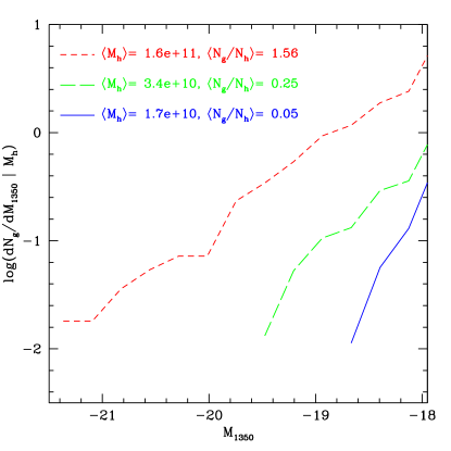
Figure 14: The simulated CLF at $z=5.5$ in three bins of halo mass; mean halo masses and occupancies within these bins are indicated. The CLF is well-approximated by a power law whose slope steepens and normalization decreases to lower masses. The mean occupancy increases with increasing halo mass as observed, but in our simulations this reflects the mass-dependence of the CLF rather than a star formation duty cycle.

If “dark” halos do not host LBGs that are experiencing a temporarily quiescent phase, then what sort of galaxies do they host? We propose that halos that are more massive than $M_{\mathrm{min}}$ but that do not host an observable galaxy preferentially host galaxies that are simply faint. In Figure 14, we illustrate this possibility through the predicted CLF at $z=5.5$ in three bins of halo mass. The halo mass bins are $1.26<M_{h}<2.5$, $2.5<M_{h}<5$, and $5<M_{h}$ in units of $10^{10}M_{\odot}$; the corresponding mean halo masses are indicated in the Figure. For each bin, we compute the predicted CLF by counting the number of galaxies as a function of absolute UV magnitude (including dust) whose host halo mass falls within that mass bin and then dividing by the number of simulated halos in that bin. Our CLF is well-approximated by a power law whose slope flattens and normalization increases with increasing halo mass. Unlike the wind-free models of Zheng et al. (2005), it does not show a bump at high luminosities corresponding to the central galaxy contribution because the scatter in the relation between halo mass and UV luminosity smooths this feature out. These CLFs have several interesting implications. First, their steep slopes imply that most halos above $10^{10}M_{\odot}$ host galaxies whose luminosities fall below current detection limits. Second, the presence of faint galaxies in massive halos (largely as satellites) explains the observation of enhanced substructure around bright galaxies at $z=4$ (Lee et al., 2006, Figure 5). Finally, integrating these functions down to the current observational limit of $M_{1350}<=-18.0$ yields the mean observable occupancy in bins of halo mass, which we find grows from 0.05 to 1.56 as the halo mass increases by a factor of 10. This finding supports the assumption of HODs that predict a lower LBG occupancy at lower halo masses (Lee et al., 2006), but within our simulations it reflects the mass dependence of the CLF rather than a halo mass-dependent star formation duty cycle.

In summary, Figures 13 and 14 show that our simulations are consistent with observed LBG occupancies of less than unity, but—given our near-unity star formation duty cycles—they predict that the “dark” halos preferentially host galaxies that are simply too faint to be observed rather than galaxies that are temporarily dusty or quiescent. Of course, scatter in the dust column and SFR at a given halo mass must contribute to the observed occupancy at some level, but our simulations suggest that these effects are not dominant. It is possible that other feedback processes such as local ionizing backgrounds (Cantalupo, 2010; Gnedin, 2010) or energy-driven outflows may be similarly successful in reproducing the observed occupancy, although momentum-driven outflows are attractive because they have already been shown to reproduce a wide variety of complementary constraints (Section 2). The important point is that there is no conflict between the observed low occupancies and the smoothly-rising SFH scenario. This interpretation makes several predictions, which we discuss in the next section.

7.3 Predictions

First, invoking strong outflows in order to explain the suppressed observed occupancy predicts that the minimum mass halo that can contribute to the observed sample $M_{\mathrm{min}}$ is larger than would be expected given the galaxy’s baryonic mass and the global baryon fraction. To illustrate this, we have determined the predicted relationship between $M_{1350}$ and baryonic mass at $z=5.5$, multiplied by $\Omega_{M}/\Omega_{b}$ to obtain the minimum mass halo that could host a galaxy with $M_{1350}$=-18 and -19, and marked these minimum halo masses with arrows in the top panel Figure 13. The actual minimum halo mass is roughly twice as large as would be expected without strong feedback (for example, Berlind et al., 2003; Zheng et al., 2005). Note that increasing our outflow strengths in order to improve the agreement with the observed colours and UV LF (Figures2 and 7) would widen this gap.

Second, mass-dependent outflows that “round off” the HOD at low masses tend to increase the minimum mass halo that hosts an average of one satellite galaxy, $M_{1}$, even more than they increase $M_{\mathrm{min}}$. Consequently, we find that the ratio $M_{1}/M_{\mathrm{min}}$ is 17–18 for both simulated LBG samples.   Zheng et al. (2005) noted that simulations that do not treat outflows predict a ratio of 14 whereas a SAM that did predicted ratios of roughly 18. By contrast, low redshift observations indicate a ratio of 18 (Zehavi et al., 2005; Zheng et al., 2007), in excellent agreement with our outflow model. These considerations suggest that galaxy clustering measurements are sensitive to the effects of galactic outflows, although further inquiry is required in order to understand how constraining these measurements are.

Third, if the galaxies living in “dark” halos are LBG “cousins” that happen to be quiescent or dusty, then the complementary galaxy fraction should be visible in optically-selected samples. Hence the smoothly-rising SFH scenario predicts that UV-selected and optically-selected samples should largely overlap. Brammer & van Dokkum (2007) used a Balmer break selection to identify samples of galaxies at $z\sim 2.4$ and 3.7 that directly test this idea. They found that, while some of their $z\sim 2.4$ sample possess red UV continua indicative of significant dust or a less active star formation phase, the majority of their $z\sim 3.7$ sample possess blue continua and would satisfy LBG colour cuts even though they were selected on the basis of their Balmer breaks. This finding argues against the existence of a significant population of quiescent or dusty B-dropout “cousins” (see also Overzier et al. 2009). Note that this conclusion is not in conflict with the observation that $\geq 80\%$ of massive ($M_{*}>5\times 10^{10}M_{\odot}$) galaxies at $z\geq 3.5$ may be too red for LBG selections (Mancini et al., 2009) because the majority of star-forming galaxies at $z\geq 4$ are not expected to be this massive–indeed, observations suggest that galaxies become increasingly low-mass and dust-free at redshifts above 3 (for example, Brammer & van Dokkum, 2007; Verma et al., 2007; Bouwens et al., 2009a, 2010a). Further exploration of optically-selected samples at $z\geq 4$ would be useful in confirming the results of Brammer & van Dokkum (2007) as their samples were rather small (23 candidates at $z\sim 4$) and lacked spectroscopic redshifts.

Fourth, the scatter in the SFR-$M_{*}$ relation should be small since short duty cycles would give rise to a significant number of galaxies that were transitioning between active and quiescent states. For example, assuming that galaxies transition between active and quiescent states on a halo dynamical time of $\approx 100$ Myr and that the active star-formation period lasts 400 Myr (Lee et al., 2009), roughly half the number of actively star-forming LBGs should be observable in a transition state below the star-forming “main sequence”. Labbé et al. (2009) measure a small scatter of $0.25$ dex at $z=7$ and do not observe a transition population even though their observations are sensitive to galaxies well below the star-forming main sequence (for example, see the inset panel in their Figure 2). These observations are difficult to reconcile with short star formation duty cycles.

Finally, we predict that the observed occupancy should not be lower for fainter samples than for brighter ones because a larger fraction of halos host faint galaxies than bright galaxies (Figure 14). This is visible in the bottom panel of Figure 13, where thin and thick curves indicate the cumulative occupancy without and with the contribution of satellite galaxies. If satellite galaxies are ignored then the occupancy, defined in this case as the fraction of halos above $M_{\mathrm{min}}$ that host at least one observable galaxy, is roughly the same for fainter and brighter samples. If satellite galaxies are included then the occupancy, now defined as $N_{g}/N_{h}(M_{h}>M_{\mathrm{min}})$, increases for fainter samples owing to the contribution of satellites. Note that this prediction is in direct conflict with a scenario in which low-mass galaxies at high redshift possess bursty SFHs reminiscent of local dwarf galaxies. Unfortunately, Lee et al. (2009) assumed a single duty cycle and did not explore this question in detail. Intriguingly, however, their brightest subsample at $z\sim 4$ prefers duty cycles of 10–50% whereas their full sample—whose clustering properties are presumably dominated by the more numerous faint galaxies—prefers longer duty cycles of 25–100% (their Figure 9), in qualitative agreement with our prediction. More detailed exploration of the luminosity dependence of the occupancy should be possible with current and upcoming data sets and would constitute a useful test of our predicted SFHs.

8 Trends at Lower Redshifts

Observations at $z<6$ indicate that galaxies eventually depart from the smoothly-rising, scale-invariant SFHs that are observed at earlier epochs. In this Section, we comment on these observations and discuss relevant physical processes that could emerge at $z<6$.

We begin by considering whether star formation is a steady-state process at all masses. The SFHs of actively star-forming galaxies more massive than $10^{9}M_{\odot}$ are likely to be predominantly smooth at all redshifts. Observations in support of this view include the tight observed scatter in the SFR-$M_{*}$ relation ($<0.3$ dex) down to $z=0$ (Noeske et al., 2007a; Brinchmann et al., 2004) and the fact that visibly merging galaxies account for less than $30\%$ of all star formation during $z\sim$0.24–0.80 (Jogee et al. 2009; see also Wolf et al. 2005).

At lower masses, evidence that dwarf galaxies experience short-lived starbursts has historically prompted many to favor generally bursty SFHs for dwarfs (Searle & Sargent, 1972). Starbursts could owe to interactions or to an irregular gas inflow rate. However, more recent studies employing larger samples have thrown the significance of starbursts in dwarfs’ SFHs into doubt. For example, Lee et al. (2009) found that dwarfs whose emission lines possess high equivalent widths live preferentially in underdense regions. This is inconsistent with the view that interaction-induced starbursts dominate dwarfs’ SFHs because interactions are more frequent in overdense regions. It suggests instead that star formation is suppressed in dwarfs that become satellite galaxies. This is expected if inflows drive star formation because inflows funnel gas preferentially onto the central galaxy. Note that we expect inflows to be smooth at $z>6$ because most observed galaxies are central galaxies (compare thin and thick curves from the bottom panel of Figure 13).

More recently, Lee et al. (2009) found that only 6% of a volume-complete sample of $\approx 300$ local dwarf galaxies are currently undergoing starbursts. Further, bursts accounted for at most one quarter of the total current star formation in their sample. Together with Jogee et al. (2009), these results indicate that star formation in the central galaxies of halos below $10^{12}M_{\odot}$ is a predominantly smooth process at all redshifts, which is a prediction of our model as well as others (for example, Guo & White, 2008; Cattaneo et al., 2010).

Departures from rising SFHs are observed after $z=2$ in two senses. First, the emergence of a bimodality in galaxy colours as early as $z=2$ (Giallongo et al., 2005) reflects the fact that many galaxies eventually cease forming stars. These “quenched” galaxies live preferentially in overdense regions (Hogg et al., 2004; Cooper et al., 2010), which supports the view that quenching owes to the onset of hot-mode accretion in halos more massive than $\approx 10^{12}M_{\odot}$ (Kereš et al., 2005, 2009), possibly coupled with extra heating from a central source (Croton et al., 2006; Cattaneo et al., 2006). These effects should be weak in current $z>6$ samples because their host halos are generally less massive than $10^{12}M_{\odot}$ (Figure 13).

Second, observations indicate that the SFRs of galaxies whose SFHs are not yet quenched decrease for $z<1$ (Noeske et al., 2007a; Pérez-González et al., 2008). This cannot be attributed to evolution in the interaction rates because observations indicate that the merger rate evolves either mildly (Cassata et al., 2005) or not at all (Lotz et al., 2008) out to $z\sim 1$. On the other hand, it occurs naturally if the gas accretion rate is assumed to trace the host halo’s growth rate because halo growth rates fall off at late times owing to cosmological expansion. Models that incorporate this effect readily yield rising SFHs at early times and decaying SFHs at late times (Davé, 2008; Bouché et al., 2009; Dutton et al., 2009).

Finally, observations indicate that the slope of the SFR-$M_{*}$ relation flattens from $\sim$unity at $z=6$ to 0.7–0.9 at $z<2$ (for example, Brinchmann et al., 2004). This departure from scale-invariance is equivalent to downsizing (Cowie et al., 1996). Our simulations predict a slope of $\approx 0.9$ at $z\leq 2$ (Davé, 2008), hence they qualitatively reproduce the observed evolution. Two effects contribute. First, the fraction of galaxies living in massive ($>10^{12}M_{\odot}$) halos increases with time and mass. If the early stages of quenching (see above) involve suppressed inflow rates and a gradual exhaustion of available gas reservoirs, then the amount of suppression should increase with time and mass. This should manifest both as an overall flattening of the SFR-$M_{*}$ relation (Davé, 2008), and as a dependence of the slope on environment. Second, feedback processes that delay gas accretion or star formation in low-mass halos flatten the predicted slope (Noeske et al., 2007b; Bouché et al., 2009). Momentum-driven outflows are a natural candidate because the mass-loading factors scale inversely with the velocity dispersion. This in turn causes gas in low-mass halos to spend most of its time suspended above the galaxy’s ISM. Outflows are also appealing because they reconcile our simulations with a wide range of complementary observations (Section 1).  Dutton et al. (2009) argued that outflows cannot change the slope of the predicted SSFR trend, but their model did not treat the possibility of outflows that do not escape from the halo.

While our simulations qualitatively reproduce the observed flattening trend, in detail they predict slightly less flattening than is observed. This could suggest either that inflows in massive halos are undersuppressed (Gabor et al., 2010), or that star formation in low-mass halos is delayed by other processes in addition to outflows. One possibility is heating by the local ionizing background within each galaxy (Cantalupo, 2010; Gnedin, 2010). Our model does not treat the local background, but it would be interesting to explore in future work.

In summary, star formation in halos below $10^{12}M_{\odot}$ is likely to be a smooth process at all redshifts, but below $z\approx$2–3 the SFRs begin to decline and the SFR-$M_{*}$ trend flattens. The emergence of declining SFRs following $z\approx 2$ owes to the decline in halo growth rates, which in turn owes to cosmological expansion. Meanwhile, the departure from scale-invariance owes to at least two effects. In massive halos, accretion shocks and AGN feedback likely suppress inflows. In low-mass halos, outflows expel cold, star-forming gas while ionizing backgrounds heat it more rapidly than it can be replaced by fresh inflows.

9 Summary

We have conducted a detailed comparison between the predictions of state-of-the-art cosmological hydrodynamic simulations including momentum-driven outflows and recent observations of reionization-epoch galaxies in order test two fundamental predictions regarding high-redshift SFHs:

1. SFHs at early times are smoothly-rising; and

2. SFH shapes are scale-invariant.

Our findings are as follows:

1. Our simulations reproduce the observed rest-frame UV luminosity function as well as its integral to current limits to within a factor of 2–3 during the epoch $z=$6–8. They also reproduce the observed stellar mass density to current limits. Either of these constraints could in principle be matched by any SFH at a single epoch, but the only smooth SFH that can account for their evolution is a rising one. This suggests that our prescriptions for star formation and feedback yield SFHs in reasonable agreement with current constraints. In detail, we find that increasing the assumed outflow mass-loading factors by $\approx$50% could bring the predicted and observed UV luminosity densities into better agreement without compromising the good agreement with the observed stellar mass density (to within the reported errors). Integrating below current detection limits, we estimate that current observations probe the brightest 30% of the total star formation and stellar mass densities at $z\geq 6$.

2. We reproduce the observed blue UV continua at $z=7$ for all but the faintest galaxies and marginally reproduce the observed bluening to lower luminosities. The UV continua of the faintest galaxies may suggest lower metallicities and a nonzero ionizing escape fraction (Bouwens et al., 2010a). We attribute the observed colour-magnitude trend to a modest level of dust reddening that increases with luminosity as seen at lower redshifts (Meurer et al., 1999; Shapley et al., 2001). This suggests that exotic stellar populations are not required in order to explain observations of galaxies brighter than $H_{160}=27.5$ at $z=7$ (Finkelstein et al., 2009; Bouwens et al., 2010a).

3. Our simulations’ relatively evolved stellar populations predict red $H_{160}-[3.6]$ colours at $z\geq 6$, augmented by dust and optical emission lines. However, the predicted colours are $\approx 0.5$ mag bluer than reported by Labbé et al. (2009). It is not clear whether resolving this discrepancy requires significantly higher mass resolution or improved observations. For the brightest galaxies, allowing the redshift and extinction to vary freely enables our models to reproduce the observed $K$–$[4.5]$ fluxes while underproducing the observed $J_{125}$ and $H_{160}$ fluxes. This suggests that the red observed $H_{160}-[3.6]$ colours may be as likely to owe to systematic error in the WFC3 as in the IRAC observations.

4. We reproduce the near-unity slope of the observed SFR-$M_{*}$ relation at all redshifts. This agreement supports a scenario in which observed reionization-epoch galaxies began forming stars at similar epochs and possess SFHs that vary only by a scale factor, which is a robust prediction of hydrodynamic simulations. We also reproduce the observed slow evolution of the SSFR, which is incompatible with constant or smoothly declining SFHs while supporting smoothly-rising SFHs (Stark et al., 2009). The predicted scatter is $\approx 0.1$dex, less than the (still remarkably tight) reported scatter of 0.25 dex. The larger observed scatter may imply a need for higher mass resolution in order to resolve the impact of minor mergers, but it may also be boosted by observational uncertainties. An offset of a factor of 2–3 between observations and predictions suggests that observationally-inferred stellar masses should be corrected for the likely impact of optical emission lines.

5. Our significantly improved treatment for the production and transport of metals predicts that observable galaxies at $z\geq 6$ possess metallicities in excess of 0.1$Z_{\odot}$. This is several times larger than our previous prediction. Increasing the assumed outflow mass-loading factors to improve the agreement between the predicted and observed UV LFs would lower these predictions by $\sim 0.1$ dex, but it would not change the fundamental result that galaxies self-enrich quite quickly. Hence we confirm that it should be possible to understand current samples without reference to Population III stars. Nevertheless, a residual fraction $10^{-3}$ of all star formation at $z=6$–8 may occur below the Population III metallicity threshold, which may eventually be visible as pair-production supernovae or GRBs.

6. There is no conflict between observations suggesting that many massive halos do not contribute to the observed samples at $z=4$–5 and the smoothly-rising SFH scenario. This is because clustering observations constrain the halo occupancy rather than the star formation duty cycle. The latter is only one of several possible interpretations of an overall occupancy that is less than unity, and our simulations disfavor it. Instead, we favor the interpretation that it reflects the scatter in the luminosity-halo mass relation. This is because strong outflows boost the scatter in the SFRs of low-mass halos, suppressing the UV luminosities of many isolated central galaxies that would be visible in the absence of outflows. Consequently, more than half of observed galaxies live in halos whose mean (observable) occupancy is less than one and the overall fraction of halos above $M_{\mathrm{min}}$ that host an observable galaxy is 0.2–0.3 as observed even though the predicted star formation duty cycle is unity. A halo occupancy in this range should thus be regarded as indicative of a high star formation duty cycle rather than a low one. This interpretation makes a number of predictions:

   1. The minimum mass for hosting an observed galaxy $M_{\mathrm{min}}$ is at least twice as large as would be expected given galaxies’ baryonic masses and the global baryon mass fraction;

   2. The minimum mass for hosting an average of two galaxies is larger than $M_{\mathrm{min}}$ by a factor of 17–18;

   3. Optically-selected and UV-selected samples should largely overlap at $z\geq 4$;

   4. The scatter in the SFR-$M_{*}$ relationship should be small, and few galaxies should be observed with suppressed SSFRs indicative of a transition between active and quiescent states;

   5. The overall occupancy for faint samples should be greater than or equal to the overall occupancy for brighter samples, in direct conflict with a picture in which lower-mass galaxies possess burstier SFHs in analogy with local dwarf galaxies.

   Each of these predictions is in tentative agreement with current observations, but we expect that more detailed analyses of current and upcoming samples will test them more thoroughly.

Further progress in understanding high-redshift SFHs will occur on both theoretical and observational fronts. On the theoretical side, it would be interesting to increase our mass resolution significantly while relaxing the assumption that wind particles temporarily decouple hydrodynamically in order to resolve feedback on small scales. Simulations of dwarf galaxy formation at low redshift tend to find burstier SFHs as the mass resolution is increased (for example, Valcke et al., 2008) owing to stochastic processes (Gerola et al., 1980), hence it is natural to suppose that similarly low-mass objects at $z\geq 6$ would also be bursty. On the other hand, dwarf galaxy SFRs are generally $<0.5M_{\odot}\mbox{yr}^{-1}$ whereas even the faintest $z=7$ galaxies indicate SFRs of $>2M_{\odot}\mbox{yr}^{-1}$; whether bursty SFRs are expected in the presence of efficient gas inflows is unclear. If so, this may improve the agreement with the observed scatter in the SFR-$M_{*}$ relation as well as the colours of low-mass galaxies (Labbé et al., 2009). Unfortunately, increasing our mass resolution is not trivial because our present simulations already probe current computational limitations. Further progress will require resimulations of a statistical sample of high-redshift galaxies (for example, Brooks et al., 2007). By contrast, incorporating stronger outflows in order to improve the agreement with the observed UV luminosity function would be trivial (aside from the computational expense), although it remains to be seen whether this would also preserve the agreement with the observed density of metals in the intergalactic medium (Oppenheimer et al., 2009b).

The impact of an inhomogeneous ionizing background warrants closer scrutiny. Our current work does not indicate that our assumption of a uniform Haardt & Madau (2001) ionizing background produces large errors in our predictions (DFO06). Nonetheless, it would be useful to study the relative roles of photoionization heating versus outflows in suppressing star formation in faint galaxies using simulations that treat the nascent ionizing background self-consistently. Preliminary work suggests that interesting nonlinear interactions exist between outflows and the ionizing background; these warrant more detailed study (Pawlik & Schaye, 2009).

A closer inquiry into the nature of our predicted HOD and its ability to reproduce clustering constraints at $z=4$–5 is in order. We have not delved into a full clustering analysis because our goal has been to demonstrate that clustering properties in the presence of mass-dependent outflows are qualitatively different than the conventional central-satellite HOD picture and have the potential to reconcile the observed duty cycle with smoothly-rising SFHs. To this end, we have already demonstrated encouraging agreement between our predictions and the observed occupancy and $M_{1}/M_{\mathrm{min}}$. A more detailed study of the CLF and its associated HOD in simulations with and without outflows would bring the impact of outflows on the HOD into sharper relief while providing a new class of template HODs for interpreting observations. Such a study would involve using our predicted HOD to populate halos from a larger-volume N-body simulation in order to provide good statistics, a task that is well beyond the scope of our current work.

On the observational side, further progress will follow from a more systematic reconstruction of the high-redshift SFR-$M_{*}$ correlation and its evolution, which are the most important observational probes of the “typical” SFH in an epoch where the SFHs of individual galaxies remain unconstrained. This involves work on three fronts: First, deeper rest-frame optical constraints on larger samples of galaxies are required in order to leverage existing UV-selected samples. Second, progress requires improved SED modeling that invokes physically-motivated SFHs (rather than, for example, instantaneous bursts) and accounts for nebular emission in order to reduce systematic errors. Third, uniform SED-fitting studies incorporating common modeling assumptions (for example, Schaerer & de Barros, 2010) will reduce artificial scatter owing to differing modeling assumptions. Because of the importance of the SFR-$M_{*}$ plot, we heartily encourage the publication of inferred physical properties order to facilitate further theoretical comparisons.

In order to gain a better understanding of the scatter in the SFR-$M_{*}$ relation as well as the implications of the low observed halo occupancy, we encourage further inquiry into the overlap between UV-selected and optically-selected samples at $z\geq 4$, following the example of Brammer & van Dokkum (2007). These studies are a strong test of our prediction that SFHs are predominantly smooth rather than bursty.

With the growing body of observational evidence that high-redshift SFHs are smooth rather than bursty and the implication that the progenitors of $V$-dropouts, for example, are visible as $i$-dropouts, it is important that SED-fitting studies account for galaxies’ hypothetical progenitors at earlier epochs in addition to their observed fluxes. For example, exponentially decaying SFHs with a decay time of 300 Myr applied to $V$-dropouts predict bright progenitor $i$-dropouts whose colours/SSFRs are observationally ruled out (unless they are very dusty, which again reinforces the need for study of optically-selected samples). For the same reason, it is now becoming possible to constrain high-redshift galaxy SFHs using statistical methods applied at multiple epochs (see, for example, Conroy & Wechsler, 2009; Maraston et al., 2010; Papovich et al., 2010). Such studies provide complementary tests of our predicted SFHs.

Finally, we have outlined a number of predictions regarding the clustering properties of faint ($M_{1350}>-20$) high-redshift galaxies that may be amenable to study using current samples (for example, from GOODS) and that should be considered in the design of upcoming Hubble and Spitzer programs to study the distant universe.

References

- Anders & Fritze-v. Alvensleben (2003) Anders, P., & Fritze-v. Alvensleben, U. 2003, A&A, 401, 1063
- Asplund et al. (2009) Asplund, M., Grevesse, N., Sauval, A. J., & Scott, P. 2009, ARA&A, 47, 481
- Berlind & Weinberg (2002) Berlind, A. A., & Weinberg, D. H. 2002, ApJ, 575, 587
- Berlind et al. (2003) Berlind, A. A., et al. 2003, ApJ, 593, 1
- Birnboim et al. (2007) Birnboim, Y., Dekel, A., & Neistein, E. 2007, MNRAS, 380, 339
- Bothwell et al. (2009) Bothwell, M. S., Kennicutt, R. C., & Lee, J. C. 2009, MNRAS, 400, 154
- Bouché et al. (2009) Bouché, N., et al. 2009, arXiv:0912.1858
- Bouwens et al. (2007) Bouwens, R. J., Illingworth, G. D., Franx, M., & Ford, H. 2007, ApJ, 670, 928
- Bouwens et al. (2009a) Bouwens, R. J., et al. 2009, ApJ, 705, 936
- Bouwens et al. (2009b) Bouwens, R. J., et al. 2009, arXiv:0909.1803
- Bouwens et al. (2009c) Bouwens, R. J., et al. 2009, arXiv:0912.4263
- Bouwens et al. (2010a) Bouwens, R. J., et al. 2010, ApJL, 708, L69
- Bouwens et al. (2010b) Bouwens, R. J., et al. 2010, arXiv:1006.4360
- Bradley et al. (2008) Bradley, L. D., et al. 2008, ApJ, 678, 647
- Brammer & van Dokkum (2007) Brammer, G. B., & van Dokkum, P. G. 2007, ApJL, 654, L107
- Brinchmann et al. (2004) Brinchmann, J., Charlot, S., White, S. D. M., Tremonti, C., Kauffmann, G., Heckman, T., & Brinkmann, J. 2004, MNRAS, 351, 1151
- Bromm & Larson (2004) Bromm, V., & Larson, R. B. 2004, ARA&A, 42, 79
- Brooks et al. (2007) Brooks, A. M., Governato, F., Booth, C. M., Willman, B., Gardner, J. P., Wadsley, J., Stinson, G., & Quinn, T. 2007, ApJL, 655, L17
- Bruzual & Charlot (2003) Bruzual, G. & Charlot, S. 2003, MNRAS, 344, 1000
- Bullock et al. (2002) Bullock, J. S., Wechsler, R. H., & Somerville, R. S. 2002, MNRAS, 329, 246
- Bunker et al. (2009) Bunker, A., et al. 2009, arXiv:0909.2255
- Calzetti et al. (2000) Calzetti, D., Armus, L., Bohlin, R. C., Kinney, A. L., Koornneef, J., & Storchi-Bergmann, T. 2000, ApJ, 533, 682
- Cantalupo (2010) Cantalupo, S. 2010, MNRAS, 403, L16
- Capak et al. (2009) Capak, P., et al. 2009, arXiv:0910.0444
- Cassata et al. (2005) Cassata, P., et al. 2005, MNRAS, 357, 903
- Castellano et al. (2009) Castellano, M., et al. 2009, arXiv:0909.2853
- Cattaneo et al. (2006) Cattaneo, A., Dekel, A., Devriendt, J., Guiderdoni, B., & Blaizot, J. 2006, MNRAS, 370, 1651
- Cattaneo et al. (2010) Cattaneo, A., Mamon, G. A., Warnick, K., & Knebe, A. 2010, arXiv:1002.3257
- Chabrier (2003) Chabrier, G. 2003, PASP, 115, 763
- Charlot & Bruzual (2007) Charlot, S. & Bruzual A., G. 2007, MNRAS, in preparation
- Chary, Stern & Eisenhardt (2005) Chary, R.-R., Stern, D., & Eisenhardt, P. 2005, ApJL, 635, L5
- Chieffi & Limongi (2004) Chieffi, A., & Limongi, M. 2004, ApJ,608, 405
- Conroy & Wechsler (2009) Conroy, C., & Wechsler, R. H. 2009, ApJ, 696, 620
- Cooper et al. (2010) Cooper, M. C., et al. 2010, arXiv:1007.1967
- Cowie et al. (1996) Cowie, L. L., Songaila, A., Hu, E. M., & Cohen, J. G. 1996, AJ, 112, 839
- Croton et al. (2006) Croton, D. J., et al. 2006, MNRAS, 365, 11
- Daddi et al. (2007) Daddi, E., et al. 2007, ApJ, 670, 156
- Davé et al. (2000) Davé, R., Gardner, J., Hernquist, L., Katz, N., & Weinberg, D. 2000, Clustering at High Redshift, 200, 173
- Davé et al. (2006) Davé, R., Finlator, K., & Oppenheimer, B. D. 2006, MNRAS, 370, 273 (DFO06)
- Davé (2008) Davé, R. 2008, MNRAS, 385, 147
- Dekel & Birnboim (2006) Dekel, A., & Birnboim, Y. 2006, MNRAS, 368, 2
- Dow-Hygelund et al. (2005) Dow-Hygelund, C. C., et al. 2005, ApJL, 630, L137
- Dunlop et al. (2007) Dunlop, J. S., Cirasuolo, M., & McLure, R. J. 2007, MNRAS, 376, 1054
- Dutton et al. (2009) Dutton, A. A., van den Bosch, F. C., & Dekel, A. 2009, arXiv:0912.2169
- Egami et al. (2005) Egami, E., et al. 2005, ApJL, 618, L5
- Elbaz et al. (2007) Elbaz, D., et al. 2007, A&A, 468, 33
- Erb et al. (2006) Erb, D. K., Shapley, A. E., Pettini, M., Steidel, C. C., Reddy, N. A., & Adelberger, K. L. 2006, ApJ, 644, 813
- Eyles et al. (2005) Eyles, L. P., Bunker, A. J., Stanway, E. R., Lacy, M., Ellis, R. S., & Doherty, M. 2005, MNRAS, 364, 443
- Eyles et al. (2007) Eyles, L. P., Bunker, A. J., Ellis, R. S., Lacy, M., Stanway, E. R., Stark, D. P., & Chiu, K. 2007, MNRAS, 374, 910
- Fan et al. (2001) Fan, X., et al. 2001, AJ, 121, 54
- Fan et al. (2006) Fan, X., Carilli, C. L., & Keating, B. 2006, ARA&A, 44, 415
- Ferguson et al. (2002) Ferguson, H. C., Dickinson, M., & Papovich, C. 2002, ApJL, 569, L65
- Finlator et al. (2006) Finlator, K., Davé, R., Papovich, C., & Hernquist, L. 2006, ApJ, 639, 672
- Finlator et al. (2007) Finlator, K., Davé, R., & Oppenheimer, B. D. 2007, MNRAS, 376, 1861
- Finlator & Davé (2008) Finlator, K., & Davé, R. 2008, MNRAS, 385, 2181
- Finkelstein et al. (2009) Finkelstein, S. L., Papovich, C., Giavalisco, M., Reddy, N. A., Ferguson, H. C., Koekemoer, A. M., & Dickinson, M. 2009, arXiv:0912.1338
- Gabor et al. (2010) Gabor, J. M., Davé, R., Finlator, K., & Oppenheimer, B. D. 2010, MNRAS, 939
- Gerola et al. (1980) Gerola, H., Seiden, P. E., & Schulman, L. S. 1980, ApJ, 242, 517
- Giallongo et al. (2005) Giallongo, E., Salimbeni, S., Menci, N., Zamorani, G., Fontana, A., Dickinson, M., Cristiani, S., & Pozzetti, L. 2005, ApJ, 622, 116
- Giavalisco & Dickinson (2001) Giavalisco, M., & Dickinson, M. 2001, ApJ, 550, 177
- Gnedin (2010) Gnedin, N. Y. 2010, arXiv:1006.1903
- Gonzalez et al. (2009) Gonzalez, V., Labbé, I., Bouwens, R. J., Illingworth, G., Franx, M., Kriek, M., & Brammer, G. B. 2009, arXiv:0909.3517
- Guo & White (2008) Guo, Q., & White, S. D. M. 2008, MNRAS, 384, 2
- Haardt & Madau (2001) Haardt, F. & Madau, P. 2001, in proc. XXXVIth Rencontres de Moriond, eds. D.M. Neumann & J.T.T. Van.
- Hogg et al. (2004) Hogg, D. W., et al. 2004, ApJL, 601, L29
- Jogee et al. (2009) Jogee, S., et al. 2009, ApJ, 697, 1971
- Johnson (2010) Johnson, J. L. 2010, MNRAS, 292
- Kennicutt (1998a) Kennicutt, R. C. 1998, ApJ, 498, 541
- Kennicutt (1998b) Kennicutt, R. C., Jr. 1998, ARA&A, 36, 189
- Kereš et al. (2005) Kereš, D., Katz, N., Weinberg, D. H., & Davé, R. 2005, MNRAS, 363, 2
- Kereš et al. (2009) Kereš, D., Katz, N., Fardal, M., Davé, R., & Weinberg, D. H. 2009, MNRAS, 395, 160
- Komatsu et al. (2010) Komatsu, E., et al. 2010, arXiv:1001.4538
- Kravtsov et al. (2004) Kravtsov, A. V., Berlind, A. A., Wechsler, R. H., Klypin, A. A., Gottlöber, S., Allgood, B., & Primack, J. R. 2004, ApJ, 609, 35
- Labbé et al. (2006) Labbé, I., Bouwens, R., Illingworth, G. D., & Franx, M. 2006, ApJL, 649, L67
- Labbé et al. (2009) Labbé, I., et al. 2009, arXiv:0911.1356
- Labbé et al. (2010) Labbé, I., et al. 2010, ApJL, 708, L26
- Lacey & Cole (1993) Lacey, C., & Cole, S. 1993, MNRAS, 262, 627
- Lai et al. (2007) Lai, K., Huang, J.-S., Fazio, G., Cowie, L. L., Hu, E. M., & Kakazu, Y. 2007, ApJ, 655, 704
- Larson (1998) Larson, R. B. 1998, MNRAS, 301, 569
- Lee et al. (2000) Lee, J. C., Salzer, J. J., Law, D. A., & Rosenberg, J. L. 2000, ApJ, 536, 606
- Lee et al. (2006) Lee, K.-S., Giavalisco, M., Gnedin, O. Y., Somerville, R. S., Ferguson, H. C., Dickinson, M., & Ouchi, M. 2006, ApJ, 642, 63
- Lee et al. (2009) Lee, K.-S., Giavalisco, M., Conroy, C., Wechsler, R. H., Ferguson, H. C., Somerville, R. S., Dickinson,
- Lee et al. (2009) Lee, J. C., Kennicutt, R. C., José G. Funes, S. J., Sakai, S., & Akiyama, S. 2009, ApJ, 692, 1305 M. E., & Urry, C. M. 2009, ApJ, 695, 368
- Lotz et al. (2008) Lotz, J. M., et al. 2008, ApJ, 672, 177
- Madau et al. (1998) Madau, P., Pozzetti, L., & Dickinson, M. 1998, ApJ, 498, 106
- Madau (1995) Madau, P. ApJ, 441, 18
- Magdis et al. (2010) Magdis, G. E., Rigopoulou, D., Huang, J.-S., & Fazio, G. G. 2010, MNRAS, 401, 1521
- Maio et al. (2010) Maio, U., Ciardi, B., Dolag, K., Tornatore, L., & Khochfar, S. 2010, arXiv:1003.4992
- Maiolino et al. (2008) Maiolino, R., et al. 2008, A&A, 488, 463
- Maraston et al. (2010) Maraston, C., Pforr, J., Renzini, A., Daddi, E., Dickinson, M., Cimatti, A., & Tonini, C. 2010, arXiv:1004.4546
- Mancini et al. (2009) Mancini, C., Matute, I., Cimatti, A., Daddi, E., Dickinson, M., Rodighiero, G., Bolzonella, M., & Pozzetti, L. 2009, A&A, 500, 705
- McKee & Ostriker (1977) McKee, C. F. & Ostriker, J. P. 1977, ApJ, 218, 148
- McLure et al. (2009) McLure, R. J., Cirasuolo, M., Dunlop, J. S., Foucaud, S., & Almaini, O. 2009, MNRAS, 395, 2196
- McLure et al. (2010) McLure, R. J., Dunlop, J. S., Cirasuolo, M., Koekemoer, A. M., Sabbi, E., Stark, D. P., Targett, T. A., & Ellis, R. S. 2010, MNRAS, 403, 960
- Meurer et al. (1999) Meurer, G. R., Heckman, T. M., & Calzetti, D. 1999, ApJ, 521, 64
- Mihos & Hernquist (1996) Mihos, J. C., & Hernquist, L. 1996, ApJ, 464, 641
- Mo et al. (1998) Mo, H. J., Mao, S., & White, S. D. M. 1998, MNRAS, 295, 319
- Murray et al. (2005) Murray, N., Quataert, E., & Thompson, T. A. 2005, ApJ, 618, 569
- Nagamine et al. (2004) Nagamine, K., Springel, V., Hernquist, L., & Machacek, M. 2004, MNRAS, 350, 385
- Neistein et al. (2006) Neistein, E., van den Bosch, F. C., & Dekel, A. 2006, MNRAS, 372, 933
- Noeske et al. (2007a) Noeske, K. G., et al. 2007, ApJL, 660, L43
- Noeske et al. (2007b) Noeske, K. G., et al. 2007, ApJL, 660, L47
- Oesch et al. (2010a) Oesch, P. A., et al. 2010, ApJL, 709, L16
- Oesch et al. (2010b) Oesch, P. A., et al. 2010, ApJL, 709, L21
- Okamoto et al. (2008) Okamoto, T., Gao, L., & Theuns, T. 2008, MNRAS, 390, 920
- Oliver et al. (2010) Oliver, S., et al. 2010, arXiv:1003.2446
- Ono et al. (2010) Ono, Y., Ouchi, M., Shimasaku, K., Dunlop, J., Farrah, D., McLure, R., & Okamura, S. 2010, arXiv:1004.0963
- Oppenheimer & Davé (2006) Oppenheimer, B. D., & Davé, R. 2006, MNRAS, 373, 1265
- Oppenheimer & Davé (2008) Oppenheimer, B. D., & Davé, R. 2008, MNRAS, 387, 577
- Oppenheimer & Davé (2009a) Oppenheimer, B. D., & Davé, R. 2009, MNRAS, 395, 1875
- Oppenheimer et al. (2009b) Oppenheimer, B. D., Davé, R., & Finlator, K. 2009, MNRAS, 396, 729
- Oppenheimer et al. (2010) Oppenheimer, B. D., Davé, R., Kereš, D., Fardal, M., Katz, N., Kollmeier, J. A., & Weinberg, D. H. 2010, MNRAS, 860
- Overzier et al. (2009) Overzier, R. A., et al. 2009, ApJ, 704, 548
- Ouchi et al. (2009) Ouchi, M., et al. 2009, ApJ, 706, 1136
- Pannella et al. (2009) Pannella, M., et al. 2009, ApJL, 698, L116
- Papovich et al. (2001) Papovich, C., Dickinson, M., & Ferguson, H. C. 2001, ApJ, 559, 620
- Papovich et al. (2010) Papovich, C., Finkelstein, S. L., Ferguson, H. C., Lotz, J. M., & Giavalisco, M. 2010, arXiv:1007.4554
- Pawlik & Schaye (2009) Pawlik, A. H., & Schaye, J. 2009, MNRAS, 396, L46
- Pentericci et al. (2009) Pentericci, L., Grazian, A., Fontana, A., Castellano, M., Giallongo, E., Salimbeni, S., & Santini, P. 2009, A&A, 494, 553
- Pérez-González et al. (2008) Pérez-González, P. G., et al. 2008, ApJ, 675, 234
- Salim et al. (2007) Salim, S., et al. 2007, ApJS, 173, 267
- Salvaterra et al. (2010) Salvaterra, R., Ferrara, A., & Dayal, P. 2010, arXiv:1003.3873
- Salpeter (1955) Salpeter, E. E. 1955, ApJ, 121, 161
- Schaerer & de Barros (2009) Schaerer, D., & de Barros, S. 2009, A&A, 502, 423
- Schaerer & de Barros (2010) Schaerer, D., & de Barros, S. 2010, arXiv:1002.1090
- Schiminovich et al. (2007) Schiminovich, D., et al. 2007, ApJS, 173, 315
- Searle & Sargent (1972) Searle, L., & Sargent, W. L. W. 1972, ApJ, 173, 25
- Shapley et al. (2001) Shapley, A. E., Steidel, C. C., Adelberger, K. L., Dickinson, M., Giavalisco, M., & Pettini, M. 2001, ApJ, 562, 95
- Springel & Hernquist (2002) Springel, V. & Hernquist, L. 2002, MNRAS, 333, 649
- Springel & Hernquist (2003) Springel, V. & Hernquist, L. 2003a, MNRAS, 339, 289
- Springel (2005) Springel, V. 2005, MNRAS, 364, 1105
- Stark et al. (2007) Stark, D. P., Ellis, R. S., Richard, J., Kneib, J.-P., Smith, G. P., & Santos, M. R. 2007, ApJ, 663, 10
- Stark et al. (2009) Stark, D. P., Ellis, R. S., Bunker, A., Bundy, K., Targett, T., Benson, A., & Lacy, M. 2009, ApJ, 697, 1493
- Storey & Hummer (1995) Storey, P. J., & Hummer, D. G. 1995,MNRAS, 272, 41
- Sutherland & Dopita (1993) Sutherland, R. S. & Dopita, M. A. 1993, ApJS, 88, 253
- Thoul & Weinberg (1996) Thoul, A. A., & Weinberg, D. H. 1996, ApJ, 465, 608
- Tornatore et al. (2007) Tornatore, L., Ferrara, A., & Schneider, R. 2007, MNRAS, 382, 945
- Trenti et al. (2009) Trenti, M., Stiavelli, M., & Michael Shull, J. 2009, ApJ, 700, 1672
- Trenti et al. (2010) Trenti, M., Stiavelli, M., Bouwens, R. J., Oesch, P., Shull, J. M., Illingworth, G. D., Bradley, L. D., & Carollo, C. M. 2010, arXiv:1004.0384
- Valcke et al. (2008) Valcke, S., de Rijcke, S., & Dejonghe, H. 2008, MNRAS, 389, 1111
- van Dokkum (2008) van Dokkum, P. G. 2008, ApJ, 674, 29 & Douglas, L. 2007, MNRAS, 377, 1024
- Verma et al. (2007) Verma, A., Lehnert, M. D., Förster Schreiber, N. M., Bremer, M. N., & Douglas, L. 2007, MNRAS, 377, 1024
- Weinberg et al. (2002) Weinberg, D. H., Hernquist, L., & Katz, N. 2002, ApJ, 571, 15
- White & Frenk (1991) White, S. D. M., & Frenk, C. S. 1991, ApJ, 379, 52
- Wolf et al. (2005) Wolf, C., et al. 2005, ApJ, 630, 771
- Yan et al. (2009) Yan, H., Windhorst, R., Hathi, N., Cohen, S., Ryan, R., O’Connell, R., & McCarthy, P. 2009, arXiv:0910.0077
- Yang et al. (2003) Yang, X., Mo, H. J., & van den Bosch, F. C. 2003, MNRAS, 339, 1057
- Yan & Windhorst (2004) Yan, H., & Windhorst, R. A. 2004, ApJL, 600, L1
- Yan et al. (2005) Yan, H., et al. 2005, ApJ, 634, 109
- Yan et al. (2006) Yan, H., Dickinson, M., Giavalisco, M., Stern, D., Eisenhardt, P. R. M., & Ferguson, H. C. 2006, ApJ, 651, 24
- Yoshida et al. (2002) Yoshida, N., Stoehr, F., Springel, V., & White, S. D. M. 2002, MNRAS, 335, 762
- Zackrisson et al. (2008) Zackrisson, E., Bergvall, N., & Leitet, E. 2008, ApJL, 676, L9
- Zheng et al. (2005) Zheng, Z., et al. 2005, ApJ, 633, 791
- Zheng et al. (2007) Zheng, Z., Coil, A. L., & Zehavi, I. 2007, ApJ, 667, 760
- Zheng et al. (2009) Zheng, W., et al. 2009, ApJ, 697, 1907
- Zehavi et al. (2005) Zehavi, I., et al. 2005, ApJ, 630, 1