A simple analytical approach to describe disease spread on a network

Abstract

We investigate the time evolution of disease spread on a network by using the concept of generations. We derive a set of equations, which can be used to determine the average epidemic size. We find a very good agreement between the analytical and simulation results. The details of approximations and the possibility of generalization or improvement are discussed.

1 Introduction

The spread of disease in a population has been the subject of extensive studies recently. This is an important field of investigation as it allows us to plan a better strategy for intervention in order to reduce the burden of an epidemic. This is, of course, an important issue with regard to the health of the populations of humans and other species.

Disease spread has been studied by a variety of different models and approaches. There are three basic types of model, namely, compartmental models [1, 2, 3, 4], network models [5, 6, 7, 8, 9, 10], and agent-based models [11, 12, 13]. Each type of model approaches the problem from a different angle and has its own level of simplifications or complexities, advantages or disadvantages. There has been a long debate on the question of which type of model can be considered as a parsimonious model to address the spread of disease (or a class of diseases) in an adequate manner. Among the above models, the compartmental model makes a full mixing assumption for the contact between individuals. The full-mixing assumption, which states that an infected individual is equally likely to spread the disease to any susceptible individual, is the basic assumption for the compartmental model, although it is possible to consider compartments with different activity levels. However, compartmental models may not be suitable for describing the initial phase of a disease outbreak when the number of infectious individuals is small and the progression of an outbreak is dominated by stochastic fluctuations. In network models, each infected individuals can transmit the disease to those individuals to which they are connected. A connection (also known as edge or link) between two individuals exists if disease transmission between them is possible. The edge is a static object in a static network model and a dynamic object in a dynamic network model or an agent-based model. To address several public health questions of import, static network models seem to be appropriate candidates to represent human interactions so long as the exact timing of transmission between two individuals is not known and that every individual’s connections over the period of one disease generation time is well represented in the network. A disease generation time is roughly equal to the incubation period plus the infectivity period of that disease. This, in fact, is the basis of contact tracing approaches in public health outbreak management in which all contacts within one disease generation are identified and tested for potential transmission. In should be noted that disease generation time is different from the generation interval, the latter being the time between when an individual is infected and the time that he/she infects someone else.

Disease spread on a network has been studied by several approaches, including the mean value reaction equation [14, 15, 16, 17, 18], the generating function formalism [19, 20], the time evolution of the generating function [21, 22], and computer simulations [23, 24]. Among these, the second approach focuses on only the final size value of an epidemic while the others study the time evolution of the disease spread.

In the following section we first present the theory behind the current calculation. This requires a short introduction to networks, the concept of generations and then the definition of different types of links and vertices. We next obtain a set of equations allowing us to find the number of different links and vertices in a given generation. We present the numerical result of this approach in the subsequent section in order to validate the approximations used in our calculations as well as to study other aspects of the disease spread on the network. Finally, we summarize the results and provide our overview on the subject, including the possibility of extensions and improvements.

2 Theory

We study the evolution of the disease spread on a network by using the notion of the generation. A network is built of vertices (nodes) representing individuals and links (edges) representing contacts between them that could potentially lead to disease transmission. We call two vertices “neighbors” if they are connected by a link. The degree of a vertex is defined as the number of links connecting the vertex to its neighbors, and the probability distribution of these degrees over the whole network is called the network’s degree distribution. A network is completely defined when we know the number of vertices and the way in which they are connected to one another. In most practical situations however, for instance, when the population is large, it is hard and not even necessary to keep track of the connectivity of vertices. One can create a network which is suitable for studying many aspect of the disease spread by respecting a minimum of requirements. The minimal requirement is to create a network that satisfies the desired degree distribution. The degree of each vertex can be assigned randomly and the vertices can be connected randomly as well provided that this minimum requirement is met; the connections in the real population can differ from this otherwise completely random network due to potential correlations between individuals, such as partnerships, friendships, etc. This is measured by the clustering coefficient and can be included in the network [25, 26].

We divide the vertices into three classes, namely susceptible, infectious, and removed classes (where removed means infectious in the past but are no longer infectious). Such models are called SIR models to indicate the three classes. An infectious vertex could infect each of its neighbors, with a probability $T$ during the entire period $\tau$ of its infectivity. In reality the infectivity is a complex function of time, depending on the type of infection, and the infectivity and susceptibility could also depend on the individuals. Here we model the infectivity by $T(t)=T\delta\left(t-\tau\right)$, which means that total force of infection is applied at time $\tau$, and we then remove the infective vertex. Normally one or more initially infected individual brings an infection to a population but here for the sake of simplicity we start our calculation with one initial infection. The first infected individual can transmit the disease to a fraction of its neighbors at time $\tau$ (the first generation). The first infected individual then belongs to the removed class and the new infective individuals are in the infective class. These new infective individuals could transmit the infection to their neighbors after a passage of time $\tau$ (the second generation). It is easy now to recognize that the spread of the infection in the network follows the concept of the generations. We have a number of infective individuals at each given generation (period of $\tau$) and these individuals are the carriers of the disease in the network in that generation. The rate of new infections at each given generation for a random network depends on the transmissibility T, the degree distribution within each class, the number of links that connect vertices in different classes and the relative populations of vertices in each classes. In the following we assume that the rate of new infections depends on the average degree of each class rather than their degree distributions and this leads to a significant simplification (we explicitly assume that all vertices within each class in a given generation have the same degree). Other generalizations will be discussed later.

We define $N_{r}^{g}$, $N_{i}^{g}$, $N_{s}^{g}$ as the number of removed, infective and susceptible individuals in a given generation $g$, respectively, and $z_{r}^{g}$, $z_{i}^{g}$, $z_{s}^{g}$ as their average degrees. Each vertex in a given class is connected to another vertex in the same or different class by an intra-link or inter-link, respectively. The total number of intra-link connections are specified as $L_{s}^{g}$, $L_{i}^{g}$, $L_{r}^{g}$ for links within the susceptible, infectious and removed classes, respectively; while the total number of inter-link connections between classes x and y are shown as $L_{xy}^{g}$, where x and y stand for the indices s, i and r, representing the three classes described earlier. Note that since $L_{xy}^{g}$ is the total number of links between classes x and y, then $L_{xy}^{g}=L_{yx}^{g}$. Finally, $N$, $z$ and $L$ are the total number of vertices, the average degree and the total number of links of the whole network, respectively. Also, we will use the subscript $\alpha$ as a generic index for r, i, s.

Because we are assuming that infectious individuals are removed in each generation, the number of infectious individuals in a generation is exactly the number of new infections in that generation, and this depends on the number of links between infectious and susceptible individuals. Each link between two vertices can be constructed from two stubs associated to the two vertices. A stub can be thought of the segment of a link emanating from each vertex; therefore, the number of stubs at a vertex is the degree of that vertex. The total number of stubs in a given compartment $\alpha$ is given by $N_{\alpha}^{g}z_{\alpha}^{g}$ of which $2L_{\alpha}^{g}$ contribute to intra-links and the rest contribute to the inter-links. It is then straightforward to establish these identities:

$$\begin{array}[]{l}{z_{r}^{g}N_{r}^{g}=2L_{r}^{g}+L_{rs}^{g}+L_{ri}^{g}}\\ {z_{i}^{g}N_{i}^{g}=2L_{i}^{g}+L_{is}^{g}+L_{ri}^{g}}\\ {z_{s}^{g}N_{s}^{g}=2L_{s}^{g}+L_{rs}^{g}+L_{is}^{g}}\end{array}$$ (1)

The above set of equations imposes a strong constraint on the number of intra- and inter-links. This set of equations allows us to find the number of inter-links in terms of the number of intra-links, the class average degree and the number of vertices in each class. The number of inter-links is important for measuring the spread of the disease in the network because an inter-link between the susceptible and infective classes may lead to a new case of infection.

The average number of intra-links for each class can be estimated in terms of $\{N_{\alpha}^{g},z_{\alpha}^{g}\}$ as follows. We consider a stub of a specific vertex in a compartment $\alpha$ and calculate the probability that this stub attaches to a stub corresponding to another vertex within the same class. The total number of stubs to which it could attach is

$$Nz-z_{\alpha}^{g}.$$ (2)

This means that this stub could in principle attach to any other stubs in the whole network except the ones belonging to the same vertex, i.e., self-loops are not allowed. The total number of stubs to which this stub could attach in its own class is

$$(N_{\alpha}^{g}-1)z_{\alpha}^{g},$$ (3)

excluding self-loops thus the probability that we searched for is given by

$$\frac{(N_{\alpha}^{g}-1)z_{\alpha}^{g}}{Nz-z_{\alpha}^{g}}.$$ (4)

This probability is in fact the average number of stubs attaching to a stub in the same class. The probability that the second stub of the given vertex attaches a stub of another vertex (excluding the stubs of the last two vertices) is then given by

$$\frac{(N_{\alpha}^{g}-2)z_{\alpha}^{g}}{Nz-2z_{\alpha}^{g}}$$ (5)

and for the $j$th stub by

$$\frac{(N_{\alpha}^{g}-j)z_{\alpha}^{g}}{Nz-jz_{\alpha}^{g}}.$$ (6)

This process can be continued until all stubs of the given vertex are exhausted or until all other vertices within the same class are chosen, or more precisely while

$$j\leq\gamma_{\alpha}^{g}=\min(N_{\alpha}^{g},z_{\alpha}^{g}).$$ (7)

The average number of intra-links associated to the given vertex is the sum over all of the above terms. The average number of intra-links is then given by

$$\bar{L}_{\alpha}^{g}=\frac{N_{\alpha}^{g}}{2}\left[\gamma_{\alpha}^{g}-\left(\frac{Nz}{z_{\alpha}^{g}}-N_{\alpha}^{g}\right)\left(\psi^{(1)}\left(\frac{Nz}{z_{\alpha}^{g}}\right)-\psi^{(1)}\left(\frac{Nz}{z_{\alpha}^{g}}-\gamma_{\alpha}^{g}\right)\right)\right]$$ (8)

where $\psi^{(1)}(x)$ is the first polygamma function defined as

$$\psi^{(n)}(x)=(-1)^{n+1}n!\sum_{j=0}^{\infty}\frac{1}{(x+j)^{n+1}}.$$ (9)

Equation (8) leads to $\bar{L}_{\alpha}^{g}\approx\frac{z_{\alpha}^{g}(N_{\alpha}^{g})^{2}}{2Nz}$ in the limit $N\gg\gamma_{\alpha}^{g}$ and when $N_{\alpha}^{g}>z_{\alpha}^{g}$.

We define $\tilde{N}_{\alpha}^{g}$ to be the number of vertices in the complement of the $\alpha$ class and $\tilde{z}_{\alpha}^{g}$ as their average degree. The average number of intra-links for the $\alpha$ class can also be calculated by the total average number of its inter-links (the second term in the following equation) as

$$\bar{L}_{\alpha}^{g}=\frac{1}{2}\left[N_{\alpha}^{g}z_{\alpha}^{g}-N_{\alpha}^{g}\left[\tilde{\gamma}_{\alpha}^{g}-\left(\frac{Nz}{\tilde{z}_{\alpha}^{g}}-\tilde{N}_{\alpha}^{g}-1\right)\left(\psi^{(1)}\left(\frac{Nz}{\tilde{z}_{\alpha}^{g}}\right)-\psi^{(1)}\left(\frac{Nz}{\tilde{z}_{\alpha}^{g}}-\tilde{\gamma}_{\alpha}^{g}\right)\right)\right]\right],$$ (10)

where $\tilde{\gamma}_{\alpha}^{g}=\min(\tilde{N}_{\alpha}^{g},\tilde{z}_{\alpha}^{g})$. The average number of intra-links can be evaluated by using (1) and (8) [or (10)].

Using $\bar{L}_{is}^{g}$and $\bar{L}_{rs}^{g}$ we can obtain the average number of new infections in each generation. However, we must take into account the finite size effect, because in a network of finite size we must take account of the possibility that two infectious individuals may be linked to the same susceptible individual. In fact, the number of new infections in the simplest scenario depends on $\bar{L}_{is}^{g}$. We define the average number of transmitting and non-transmitting links from the infectious compartment to be $\bar{\lambda}^{g}=T\bar{L}_{is}^{g}$ and $\bar{\lambdabar}^{g}=(1-T)\bar{L}_{is}^{g}$, respectively. The number of new infections can be obtained by assigning the transmitting links to the susceptible vertices. The first link makes a contribution of one to the new infections. The probability that the second link is attached to another vertex is roughly proportional to

$$\frac{(N_{s}^{g}-1)z_{s}^{g}}{N_{s}^{g}z_{s}^{g}}=\frac{N_{s}^{g}-1}{N_{s}^{g}},$$ (11)

and this in fact is the contribution of the second link to the average number of new infections. We assume that all susceptible vertices have the same degree, which is a good approximation when the degree distribution is narrow; we discuss the more general case later. The contribution of the $j$th link is then given by

$$\frac{N_{s}^{g}-\bar{n}_{j-1}}{N_{s}^{g}},$$ (12)

where $\bar{n}_{j-1}$ is the average number of new infections after assigning $(j-1)$ links. The average number of the new infections after assigning the $j$th links is

$$\bar{n}_{j}=\bar{n}_{j-1}+\frac{N_{s}^{g}-\bar{n}_{j-1}}{N_{s}^{g}}.$$ (13)

The number of new infections after assigning all transmitting links is then given by

$$\bar{N}_{i}^{g+1}=\frac{1-\beta_{g}^{\bar{\lambda}^{g}}}{1-\beta_{g}},$$ (14)

where $\beta_{g}=1-\frac{1}{N_{s}^{g}}$. It is straightforward to show that

$$\bar{N}_{i}^{g+1}=\bar{\lambda}^{g}-\frac{\bar{\lambda}^{g}\left(\bar{\lambda}^{g}-1\right)}{2N_{s}^{g}}$$ (15)

where $N_{s}^{g}\gg\bar{\lambda}^{g}$, which means that the average number of new infections is approximately equal to the number of transmitting links in such a situation and the correction to this is given by $\frac{(\bar{\lambda}^{g})^{2}}{2N_{s}^{g}}.$ We point out that in deriving the above equation we ignore the requirement that the infectious links emitted from one specific vertex cannot connect to the same susceptible vertex (repeated links). We may take this effect into account but the resulting formula does not show any significant difference.

It is possible to extend the above equation to the case that the degree distribution is very asymmetric with respect to the average degree

$$\bar{N}_{i}^{g+1}=\sum_{k}\bar{N}_{i}^{g+1}(k),$$ (16)

where

$$\bar{N}_{i}^{g+1}(k)=\left\{\begin{array}[]{ccc}{\frac{1-\beta_{g}(k)^{\bar{\lambda}^{g}(k)}}{1-\beta_{g}(k)}}&{,}&{\bar{\lambda}^{g}(k)>1}\\ {\bar{\lambda}^{g}(k)}&{,}&{\bar{\lambda}^{g}(k)<1}\end{array}\right\},$$ (17)

$\beta_{g}(k)=1-\frac{1}{N_{s}^{g}p_{s}^{g}(k)}$ and $\bar{\lambda}^{g}(k)=\frac{\bar{\lambda}^{g}kp_{s}^{g}(k)}{z_{s}^{g}}$.

An estimate for the average degree of each class completes the set of equations which are required for the time evolution of the disease on the network. This is similar to our earlier calculations presented in Noel et al. [18]. Because vertices with high degree are more likely to receive infection during an epidemic process, we would expect the average degree of the susceptible class to be less than the average degree of the infective and removed class, and this is of importance in describing the time evolution of the disease.

The first infection is chosen randomly so that the probability that it has degree $k$ is given by $\Delta\tilde{p}_{1}(k)=p(k)$ where $p(k)$ is the degree distribution of the network. We consider the first chosen vertex as being removed. The new degree distribution of the network remaining after removing the first vertex is $p_{1}(k)=p(k)$ because of the choice made for the first vertex. Now we pick the second vertex by choosing a random stub. The new vertex could be one of the neighbors of the first vertex in one of the networks, which is constructed by knowing the degree distribution. The probability that the second vertex has degree $k$ is given by $\Delta\tilde{p}_{2}(k)=\frac{p_{1}(k)k}{z_{1}}$. This means that the degree distribution of removed vertices is $\tilde{p}_{2}(k)=\frac{\Delta\tilde{p}_{1}(k)+\Delta\tilde{p}_{2}(k)}{2}$ and so the degree distribution of the remaining vertices can be written as $(N-2)p_{2}(k)=Np(k)-2\tilde{p}_{2}(k)$. The degree distribution of the $j$th chosen vertex is $\Delta\tilde{p}_{j}(k)=\frac{p_{j}(k)k}{z_{j}}$ and in the same manner, the degree distribution of the removed and remaining vertices are given by

$$\begin{array}[]{l}{\tilde{p}_{j}(k)=\frac{\sum_{l=1}^{j}\Delta\tilde{p}_{l}(k)}{j}}\\ {p_{j}(k)=\frac{Np(k)-j\tilde{p}_{j}(k)}{N-j}}.\end{array}$$ (18)

The average degree of the removed class is $\bar{z}_{r}^{g}=\tilde{z}_{j}=\sum_{k}\tilde{p}_{j}(k)k$ when $j=\bar{N}_{r}^{g}$. The average degree of the infective class is $\bar{z}_{i}^{g}=\frac{\left[(j+j^{\prime})\tilde{z}_{j+j^{\prime}}-j\tilde{z}_{j}\right]}{j^{\prime}}$ when $j=\bar{N}_{r}^{g}$and $j^{\prime}=\bar{N}_{i}^{g}$. Finally the average degree of the susceptible class is $\bar{z}_{s}^{g}=z_{j}=\sum_{k}p_{j}(k)k$ when $j=\bar{N}_{s}^{g}$. We point out that in the derivation of the above result, we assume that all vertices are connected to each other and this might not be true for a general network.

Now we are in a position to estimate the effect of non-transmitting links on the reduction of $N_{s}^{g}$. We call the total number of non-transmitting links $\Lambda^{g}=\bar{\lambdabar}^{g}+L_{rs}^{g}$ and the degree distribution of susceptible $P_{0}^{g}(k)=p_{s}^{g}(k)$. Assigning the first non-transmitting link without removing the vertex changes the degree distribution to

$$N_{s}^{g}P_{1}^{g}(k)=N_{s}^{g}P_{0}^{g}(k)+\frac{P_{0}^{g}(k+1)(k+1)}{Z_{0}^{g}}-\frac{P_{0}^{g}(k)k}{Z_{0}^{g}}.$$ (19)

The second and third terms in the above equation are the contribution of moving a vertex from $k+1\to k$ and $k\to k-1$ because of removing one stub. It is straightforward to show that after assigning all links,

$$N_{s}^{g}P_{\Lambda^{g}}^{g}(k)=N_{s}^{g}P_{0}^{g}(k)+\sum_{j=0}^{\Lambda^{g}-1}\frac{P_{j}^{g}(k+1)(k+1)}{Z_{j}^{g}}-\frac{P_{j}^{g}(k)k}{Z_{j}^{g}}$$ (20)

is the effective degree distribution of the susceptible class after assigning all non-transmitting links. The total number of degree zero vertices is then simply given by $N_{s}^{g}P_{\Lambda^{g}}^{g}(0)$, which should be subtracted from $N_{s}^{g}$ in (14). One can either use the effective degree distribution in (16) to take the effect of non-transmissible links into account. Note that the total number of degree zero vertices is not the only contribution to the reduction of the number of susceptible vertices, which can be reached by transmitting links. Small components make a very important contribution especially if the average degree is low or if the degree distribution has significant value in the low degree region.

3 Numerical results

Here we present our numerical results, which are mainly the solution of (1) - (20) together with the equations for the average degree of the classes. The first part of our numerical results focuses on the justification of the approximations introduced in the previous sections. We compare our analytical results against simulations for different types of networks to ensure their validity. We examine our analytical results for two distributions, namely Poisson $p(k)=\frac{z^{k}e^{-z}}{k!}$, and exponential $p(k)\propto e^{\kappa k}$ (with $z=10$ and $\kappa=10$ for all figures).

The Poisson distribution corresponds to homogeneous mixing and is in a sense the easiest example because the network is connected and the probability of a small outbreak is small. In an exponential distribution, there are many vertices of small degree and there is a higher probability that the graph will include small components which would lead to small disease outbreaks. Since we wish to describe the evolution of disease spread for large epidemics, we should discard the simulations that produce only small outbreaks. Keeping the small outbreak simulations would lower the disease curve later in the progress of the epidemic. In the figures of this section, we have incorporated the correction of discarding the simulations giving only small outbreaks.

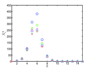
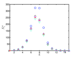
Figure 1 shows the average number of intra-links for the removed (left panel) and infectious (right panel) classes in terms of generations. The results are for the Poisson distribution, $T=0.3$ and $N=1000$. The plus signs show the direct outcome of simulation. The circles and triangles are the outputs of (8) and (10) respectively, using the number of vertices and average degree as simulation inputs. The diamonds are the result of (8) using only the number of vertices given by simulation as input. The average degree is calculated by the analytical formula of the previous section.

Figure 1: The average number of intra-link for the removed (left panel) and infectious (right panel) classes in terms of generations. The results are for the Poisson distribution, $T=0.3$ and $N=1000$.

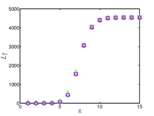
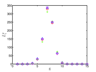
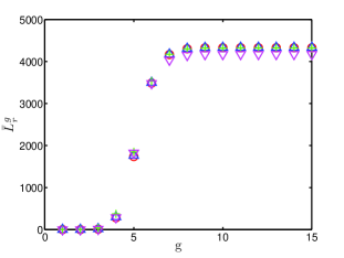
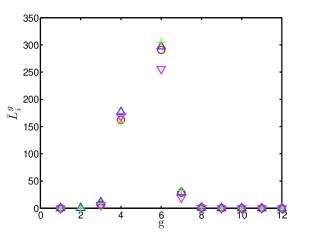
Figure 2 shows the same result for an exponential network. The main difference between the diamonds and the other results comes from the average degree given by the analytical formula (see Figure 3 and the related discussion). In fact the good agreement between plus signs, triangles and circles confirms the validity of equations (8) and (10).

Figure 2: The average number of intra-link for the removed (left panel) and infectious (right panel) classes in terms of generations. The results are for the exponential distribution, $T=0.3$ and $N=1000$.

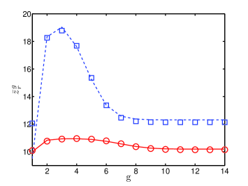
We depict the average degree of the removed class in terms of generations in Figure 3. The solid (Poisson) and dashed (exponential) lines present the analytical results and the circles (Poisson) and squares (exponential) present the simulation results. It is interesting to note the significant variation of average degree for the exponential degree distribution. This is mainly due to the width of the degree distribution. Moreover, the significant difference between the analytical and simulation results for the exponential degree distribution during the first generation is due to the exclusion of small outbreaks.

Figure 3: The average degree of the removed class in terms of generations. The solid (Poisson) and dashed (exponential) lines represent the analytical results and the circles (Poisson) and squares ( exponential) represent the simulation results.

We depict in Figure 4 the number of new infections and the average number of transmitting links for exponential (left panel) and Poisson (right panel) degree distributions for the same parameters as in previous figures. The circles present the average number of transmitting links, the squares and plus signs are the number of new infections calculated by the analytical formula (14) and obtained by simulations, respectively, before implementing the corrections that were derived analytically in equations (16) and (20). The disagreement between the simulation and the analytical results for the exponential graph is partly due to the presence of vertices of very high degree in the network or, more precisely, the asymmetry of the degree distribution with respect to the mean degree. It is straightforward to show that the majority of the stubs for an exponential graph belong to vertices with degree equal to or higher than the average degree (35% percent of vertices have 70% of the stubs for the current exponential graph). This means that the chance of multi-targeting a high degree vertex is larger compared to other vertices and this effect can reduce the average number of new infections compared to what our analytical formula (14) predicts. This is taken care of by the equation (16) and the result is shown by the triangles. The change is very small for the Poisson network because of the symmetry of the degree distribution about the average degree and also because of the small width of the degree distribution. The inclusion of the non-transmitting links ($L_{rs}^{g}$ and $\bar{\lambdabar}_{g}$) can be important when the average degree is low or when the degree distribution has a heavy tail near the origin. These links in fact can exclude many vertices by targeting their stubs and reduce the effective $N_{s}^{g}$ that the transmitting links can target. Our calculations based on equations (16) and (20) are depicted by diamonds. The effect of equation (20) might be more important for lower values of transmissibility when the number of consumed susceptible vertices due to non-transmitting links is large.

Figure 4: The number of new infections and the average number of transmitting links for exponential (left panel) and Poisson (right panel) for the same parameters as previous figures. The circles represent the average number of the transmitting links. The squares, triangles and diamonds are the number of the new infections calculated by analytical formulas. The plus signs correspond to simulation results.

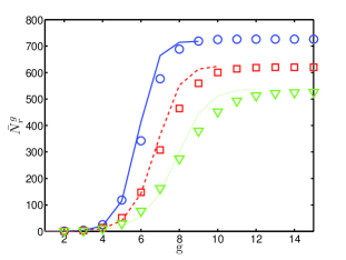
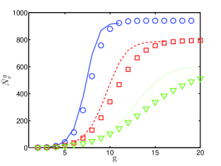
Now that we have confirmed the validity of the equations introduced earlier, we can begin solving them together to obtain the average epidemic size as a function of the generation. We start with one infection which means, $N_{r}^{0}=0$, $N_{i}^{0}=1$, $N_{s}^{0}=N-1$ and $\bar{L}_{is}^{0}=z$. Using these initial conditions we can calculate the number of transmitting links $\bar{\lambda}^{0}$and then $N_{i}^{1}$. The procedure can easily be continued to the end of the epidemic. In Figure 5 we show the average number of removed vertices as a function of generation for the exponential (left panel) and Poisson (right panel) at $T=0.15$, 0.2 and 0.3. The contribution of the small components is removed from the simulation results as they shift the mean number of removed vertices to a lower value. This size can be found simply by looking at the spectrum of component size. The difference between the analytical and simulation results is partly due to the initial stage of the simulated epidemics during which the stochastic behaviour of the outbreaks in different computer runs before entering to the large-scale epidemic have different time lengths.

Figure 5: The average number of removed vertices as a function of generation for the exponential (left panel) and Poisson (right panel) at $T=0.15$, 0.2 and 0.3. The lines and points are the analytical and simulation results respectively.

4 Conclusions and Discussion

We have presented a new approach, which describe the time evolution of the disease spread on a network. We obtain a set of equations, which determine the number of different links in each generation. This step is very important because different links have their own roles in disease spread. Different types of approximation are discussed and their validity is tested by simulation.

This approach can be extended easily to continuous time. Finding the appropriate dimension of a finite size network, which defines the number of nth neighbors, is a crucial step in this regard. One can also extend the approach to evaluate the probability of different outbreak sizes instead of the average outbreak size. The time evolution of the degree distribution for different compartments needs more attention. This requires a serious analysis of the effect of small components in the network. Knowing the relation between the average degree and the size of a component is a crucial element of this task.

References

- [1] N. T. J Bailey, The Mathematical Theory of Infection Disease and its applications (Hafner Press, New York, 1975).
- [2] R. M. Anderson and R. M. May, Infectious Disease of Humans (Oxford University Press, Oxford, 1991).
- [3] F. Brauer, P. van den Driessche and J. Wu (editors), Mathematical Epidemiology (Lecture Notes in Mathematics, Mathematical Biosciences subseries 1945, Springer, 2008).
- [4] H. W. Hethcote, SIAM Rev. 42, 599 (2000).
- [5] C. Moore and M.E.J. Newman, Phys. Rev. E 61, 5678 (2000).
- [6] M. Kuperman and G. Abramson, Phys. Rev. Lett. 86, 2909 (2001).
- [7] R. Pastor-Satorras and A. Vespignani, Phys. Rev. Lett. 86, 3200 (2001).
- [8] Y. Moreno, R. Pastor-Satorras, and A. Vespignani, Euro. Phys. Jour. B , 26, 521 (2002).
- [9] C.P. Warren, L.M. Sander, and I. Sokolov, Physica A: Stat. Mech. and its App. 325, Pages 1 (2003).
- [10] C. P. Warren, L. M. Sander, I. Sokolov, C. Simon, and J. Koopman, Math. Bioscie. 208, 205 (2007).
- [11] T.C. Schelling, Micromotives and macrobehavior (New York, Norton 1978).
- [12] G. Hartvigsen, J. M. Dresch, A. L. Zielinsk, A. J. Macla and C. C. Leary, J. Theor. Biol. 246, 205 (2007).
- [13] T. Gross, G. J. Dommar D
- [14] G. Szabó, Phys. Rev. E 62, 7474, (2000).
- [15] R. Pastor-Satorras and A. Vespignani, Phys. Rev. Lett. 86, 3200 (2001).
- [16] R. Pastor-Satorras and A. Vespignani, Phys. Rev. E 63, 066117-1 (2001).
- [17] M. Barthélemy , et al, J. Theor. Biol. 235, 275 (2005).
- [18] E. Volz, Journal of Mathematical Biology, 56 3 2008; E. Volz and L. A. Meyers, Proceedings of the Royal Society, Series B. 274 1628, 2007.
- [19] M. E. J. Newman, Phys. Rev. E 66, 016128-1 (2002).
- [20] L. A. Meyers, M. E. J. Newman and B. Pourbohloul, J. Theor. Biol. 240, 400 (2006).
- [21] M. Marder, Phys. Rev. E 75, 066103 (2007).
- [22] P.-A. Nöel, B. Davoudi, L. J. Dubé and B. Pourbohloul, Phys. Rev. E 79, 026101 (2008).
- [23] Marcelo Kupermanand Guillermo Abramson, Phys. Rev. Lett. 86, 2909 (2001).
- [24] L. K. Gallos and P. Argyrakis, Physica A 330, 117 (2003).
- [25] M. E. J. Newman, Phys. Rev. E 68, 026121 (2003).
- [26] D. J. Watts and S. H. Strogatz, Nature 393, 440 (1998).