Temporal Link Prediction using Matrix and Tensor Factorizations

Abstract

The data in many disciplines such as social networks, web analysis, etc. is link-based, and the link structure can be exploited for many different data mining tasks. In this paper, we consider the problem of temporal link prediction: Given link data for times 1 through $T$, can we predict the links at time $T+1$? If our data has underlying periodic structure, can we predict out even further in time, i.e., links at time $T+2$, $T+3$, etc.? In this paper, we consider bipartite graphs that evolve over time and consider matrix- and tensor-based methods for predicting future links. We present a weight-based method for collapsing multi-year data into a single matrix. We show how the well-known Katz method for link prediction can be extended to bipartite graphs and, moreover, approximated in a scalable way using a truncated singular value decomposition. Using a CANDECOMP/PARAFAC tensor decomposition of the data, we illustrate the usefulness of exploiting the natural three-dimensional structure of temporal link data. Through several numerical experiments, we demonstrate that both matrix- and tensor-based techniques are effective for temporal link prediction despite the inherent difficulty of the problem. Additionally, we show that tensor-based techniques are particularly effective for temporal data with varying periodic patterns.

Author Addresses: D. Dunlavy, Sandia National Laboratories, Albuquerque, NM 87123-1318, dmdunla@sandia.gov. T. Kolda, Sandia National Laboratories, Livermore, CA 94551-9159, tgkolda@sandia.gov. E. Acar, TUBITAK-UEKAE, Gebze, Turkey evrim.acar@bte.tubitak.gov.tr.

1 Introduction

The data in different analysis applications such as social networks, communication networks, web analysis, and collaborative filtering consists of relationships, which can be considered as links, between objects. For instance, two people may be linked to each other if they exchange emails or phone calls. These relationships can be modeled as a graph, where nodes correspond to the data objects (e.g., people) and edges correspond to the links (e.g., a phone call was made between two people). The link structure of the resulting graph can be exploited to detect underlying groups of objects, predict missing links, rank objects, and handle many other tasks [Getoor and Diehl (2005)].

Dynamic interactions over time introduce another dimension to the challenge of mining and predicting link structure. Here we consider the task of link prediction in time. Given link data for $T$ time steps, can we predict the relationships at time $T+1$? This problem has been considered in a variety of contexts [Hasan et al. (2006), Liben-Nowell and Kleinberg (2007), Sarkar et al. (2007)]. Collaborative filtering is also a related task, where the objective is to predict interest of users to objects (movies, books, music) based on the interests of similar users [Liu and Kou (2007), Koren et al. (2009)]. The temporal link prediction problem is different from missing link prediction, which has no temporal aspect and where the goal is to predict missing connections in order to describe a more complete picture of the overall link structure in the data [Clauset et al. (2008)].

We extend the problem of temporal link prediction stated above to the problem of periodic temporal link prediction. For such problems, given link data for $T$ time steps, can we predict the relationships at times $T+1,T+2,\dots,T+L$, where $L$ is the length of the periodic pattern? Such problems often arise in communication networks, such as e-mail and network traffic data, where weekly or monthly interaction patterns abound. If we can discover a temporal pattern in the data, temporal forecasting methods such as Holt-Winters [Chatfield and Yar (1988)] can be used to make predictions further out in time.

Time-evolving link data can be organized as a third-order tensor, or multi-dimensional array. In the simplest case, we can define a tensor $\bm{\mathscr{{Z}}}$ of size $M\times N\times T$ such that

$$\bm{\mathscr{{Z}}}(i,j,t)=\begin{cases}1&\text{if object $i$ links to object $j$ at time $t$},\\ 0&\text{otherwise}.\end{cases}$$

It is also possible to use weights to indicate the strength of the links. The goal is to predict the links at time $T+1$ or for a period time $T+1,\dots,T+L$ by analyzing the link structure of $\bm{\mathscr{{Z}}}$.

Figure 1 presents an illustration of such temporal link data for the 1991–2000 DBLP bibliometric data set, which contains publication data for a large number of professional conferences in areas related to computer science (described in more detail in §4). The plot depicts the patterns of links between authors and conferences over time, with blue dots denoting the links (i.e., values of 1 as defined above).

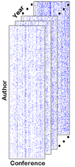
Figure 1: DBLP Data for 1991–2000.

We consider both matrix- and tensor-based methods for link prediction. For the matrix-based methods, we collapse the data into a single matrix by summing (with and without weights) the matrices corresponding to the time slices. As a baseline, we consider a low-rank approximation as produced by a truncated singular value decomposition (TSVD). Next, we consider the Katz method [Katz (1953)] (extended to bipartite graphs), which has proven to be highly accurate in previous work on link prediction [Huang et al. (2005), Liben-Nowell and Kleinberg (2007), Huang and Lin (2009)]; however, it is not always clear how to make the method scalable. Therefore, we present a novel scalable technique for computing approximate Katz scores based on a truncated spectral decomposition (TKatz). For the tensor-based methods, we consider the CANDECOMP/PARAFAC (CP) tensor decomposition [Carroll and Chang (1970), Harshman (1970)], which does not collapse the data but instead retains its natural three-dimensional structure. Tensor factorizations are higher-order extensions of matrix factorizations that capture the underlying patterns in multi-way data sets and have proved to be successful in diverse disciplines including chemometrics, neuroscience and social network analysis [Acar and Yener (2009), Kolda and Bader (2009)]. Moreover, CP yields a highly interpretable factorization that includes a time dimension. In terms of prediction, the matrix-based methods are limited to temporal prediction for a single time step, whereas CP can be used in solving both single step and periodic temporal link prediction problems.

There are many possible applications for link prediction, such as predicting the web pages a web surfer may visit on a given day based on past browsing history, the places that a traveler may fly to in a given month, or the patterns of computer network traffic. We consider two applications for link prediction. First, we consider computer science conference publication data with a goal of predicting which authors will publish at which conferences in year $T+1$ given the publication data for the previous $T$ years. In this case, we assume we have $M$ authors and $N$ conferences. All of the methods produce scores for each $(i,j)$ author-conference pair for a total of $MN$ prediction scores for year $T+1$. For large values of $M$ or $N$, computing all possible scores is impractical due to the large memory requirements of storing all $MN$ scores. However, we note that it is possible to easily compute subsets of the scores. For example, these methods can answer specific questions such as “Who is most likely to publish at the KDD conference next year?” or “Where is Christos Faloutsos most likely to publish next year?” using only $O(M+N)$ memory. This is how we envision link prediction methods being used in practice. Second, we consider the problem of how to predict links when periodic patterns exist in the data. For example, we consider a simulated example where data is taken daily over ten weeks. We should be able to recognize, for example, weekday versus weekend patterns and use those in making predictions. If we consider a scenario of users accessing various online services, we should be able to differentiate between services that are heavily accessed on weekdays (e.g., corporate email) versus those that are used mostly on weekends (e.g., entertainment services).

1.1 Our Contributions

The main contributions of this paper can be summarized as follows:

• Weighted methods for collapsing temporal data into a matrix are shown to outperform straight summation (inspired by the results in [Sharan and Neville (2008)]) in the case of single step temporal link prediction.

• The Katz method is extended to the case of bipartite graphs and its relationship to the matrix SVD is derived. Additionally, using the truncated SVD, we devise a scalable method for calculating a “truncated” Katz score.

• The CP tensor decomposition is applied to temporal data. We provide both heuristic- and forecasting-based prediction methods that use the temporal information extracted by CP.

• Matrix- and tensor-based methods are compared on DBLP bibliometric data in terms of link prediction performance and relative expense.

• Tensor-based methods are applied to periodic temporal data with multiple period patterns. Using a forecasting-based prediction method, it is shown how the method can be used to predict forward in time.

1.2 Notation

Scalars are denoted by lowercase letters, e.g., $a$. Vectors are denoted by boldface lowercase letters, e.g., ${\bm{\mathbf{{a}}}}$. Matrices are denoted by boldface capital letters, e.g., ${\bm{\mathbf{{A}}}}$. The $r$th column of a matrix ${\bm{\mathbf{{A}}}}$ is denoted by ${\bm{\mathbf{{a}}}}_{r}$. Higher-order tensors are denoted by boldface Euler script letters, e.g., $\bm{\mathscr{{Z}}}$. The $t$th frontal slice of a tensor $\bm{\mathscr{{Z}}}$ is denoted ${\bm{\mathbf{{Z}}}}_{{t}}$. The $i$th entry of a vector ${\bm{\mathbf{{a}}}}$ is denoted by ${\bm{\mathbf{{a}}}}({i})$, element $(i,j)$ of a matrix ${\bm{\mathbf{{A}}}}$ is denoted by ${\bm{\mathbf{{A}}}}(i,j)$, and element $(i,j,k)$ of a third-order tensor $\bm{\mathscr{{Z}}}$ is denoted by $\bm{\mathscr{{Z}}}(i,j,k)$.

1.3 Organization

The organization of this paper is as follows. Matrix techniques are presented in §2, including a weighted method for collapsing the tensor into matrix in §2.1, the TSVD method in §2.2, and the Katz and TKatz methods in §2.3. The CP tensor technique is presented in §3. Numerical results on the DBLP data set are discussed in §4 and on simulated periodic data in §5. We discuss related work in §6. Conclusions and future work are discussed in §7.

2 Matrix Techniques

We consider different matrix techniques by collapsing the matrices over time into a single matrix. In §2.1, we present two techniques (unweighted and weighted) for combining the multi-year data into a single matrix. In §2.2, we present the technique of using a truncated SVD to generate link scores. In §2.3, we extend the Katz method to bipartite graphs and show how it can be computed efficiently using a low-rank approximation.

2.1 Collapsing the data

Suppose that our data set consists of matrices ${\bm{\mathbf{{Z}}}}_{{1}}$ through ${\bm{\mathbf{{Z}}}}_{{T}}$ of size $M\times N$ and the goal is to predict ${\bm{\mathbf{{Z}}}}_{{T+1}}$. The most straightforward way to collapse that data into a single $M\times N$ matrix ${\bm{\mathbf{{X}}}}$ is to sum all the entries across time, i.e.,

$${\bm{\mathbf{{X}}}}(i,j)=\sum_{t=1}^{T}{\bm{\mathbf{{Z}}}}_{{t}}(i,j).$$ (1)

We call this the collapsed tensor (CT) because it collapses (via a sum) the entries of the tensor $\bm{\mathscr{{Z}}}$ along the time mode. This is similar to the approach in [Liben-Nowell and Kleinberg (2007)].

We propose an alternative approach to collapsing the tensor data, motivated by [Sharan and Neville (2008)], where the link structure is damped backward in time according to the following formula:

$${\bm{\mathbf{{X}}}}(i,j)=\sum_{t=1}^{T}(1-\theta)^{T-t}\;{\bm{\mathbf{{Z}}}}_{{t}}(i,j).$$ (2)

The parameter $\theta\in(0,1)$ can be chosen by the user or according to experiments on various training data sets. We call this the collapsed weighted tensor (CWT) because the slices in the time mode are weighted in the sum. This gives greater weight to more recent links. See Figure 2 for a plot of $f(t)=(1-\theta)^{T-t}$ for $\theta=0.2$ and $T=10$.

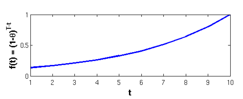
Figure 2: Plot of the decay function $f(t)=(1-\theta)^{T-t}$ for $\theta=0.2$ and $T=10$.

The numerical results in §4 demonstrate improved performance using CWT versus CT.

2.2 Truncated SVD

One of the methods compared in this paper is a low-rank approximation of the matrix ${\bm{\mathbf{{X}}}}$ produced by (1) or (2). Specifically, suppose that the compact SVD of ${\bm{\mathbf{{X}}}}$ is given by

$${\bm{\mathbf{{X}}}}={\bm{\mathbf{{U}}}}\bm{\Sigma}{\bm{\mathbf{{V}}}}^{{\sf T}},$$ (3)

where $R$ is the rank of ${\bm{\mathbf{{X}}}}$, ${\bm{\mathbf{{U}}}}$ and ${\bm{\mathbf{{V}}}}$ are orthogonal matrices of sizes $M\times R$ and $N\times R$, respectively, and $\bm{\Sigma}$ is a diagonal matrix of singular values $\sigma_{1}>\sigma_{2}>\cdots>\sigma_{R}>0$. It is well known that the best rank-$K$ approximation of ${\bm{\mathbf{{X}}}}$ is then given by the truncated SVD

$${\bm{\mathbf{{X}}}}\approx{\bm{\mathbf{{U}}}}_{K}\bm{\Sigma}_{K}{\bm{\mathbf{{V}}}}_{K},$$ (4)

where ${\bm{\mathbf{{U}}}}_{K}$ and ${\bm{\mathbf{{V}}}}_{K}$ comprise the first $K$ columns of ${\bm{\mathbf{{U}}}}$ and ${\bm{\mathbf{{V}}}}$ and $\bm{\Sigma}_{K}$ is the $K\times K$ principal submatrix of $\bm{\Sigma}$. We can write (4) as a sum of $K$ rank-1 matrices:

$${\bm{\mathbf{{X}}}}\approx\sum_{k=1}^{K}\sigma_{k}{\bm{\mathbf{{u}}}}_{k}{\bm{\mathbf{{v}}}}_{k}^{{\sf T}},$$

where ${\bm{\mathbf{{u}}}}_{k}$ and ${\bm{\mathbf{{v}}}}_{k}$ are the $k$th columns of ${\bm{\mathbf{{U}}}}$ and ${\bm{\mathbf{{V}}}}$ respectively. The TSVD is visualized in Figure 3.

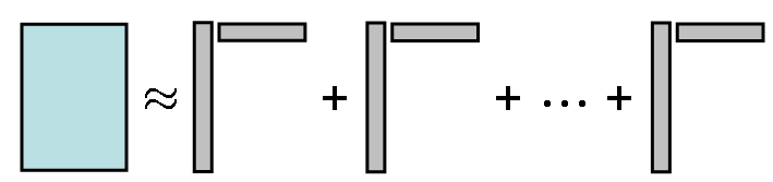
Figure 3: Illustration of the matrix TSVD.

A matrix of scores for predicting future links can then be calculated as

$${\bm{\mathbf{{S}}}}={\bm{\mathbf{{U}}}}_{K}\bm{\Sigma}_{K}{\bm{\mathbf{{V}}}}_{K}.$$ (5)

We call these the Truncated SVD (TSVD) scores. Low-rank approximations based on the matrix SVD have proven to be an effective technique in many data applications; latent semantic indexing [Dumais et al. (1988)] is one such example. This technique is called “low-rank approximation: matrix entry” in [Liben-Nowell and Kleinberg (2007)].

2.3 Katz

The Katz measure [Katz (1953)] is arguably one of the best link predictors available because it has been shown to outperform many other methods [Liben-Nowell and Kleinberg (2007)]. Suppose that we have an undirected graph $G(V,E)$ on $P=|V|$ nodes. Then the Katz score of a potential link between nodes $i$ and $j$ is given by

$${\bm{\hat{\mathbf{{S}}}}}(i,j)=\sum_{\ell=1}^{+\infty}\beta^{\ell}|\text{path}^{(\ell)}_{i,j}|,$$ (6)

where $|\text{path}^{(\ell)}_{i,j}|$ is the number of paths of length $\ell$ between nodes $i$ and $j$, and $\beta\in(0,1)$ is a user-defined parameter controlling the extent to which longer paths are penalized.

The Katz scores for all pairs of nodes can be expressed in matrix terms as follows. Let ${\bm{\hat{\mathbf{{X}}}}}$ be the $P\times P$ symmetric adjacency matrix of the graph. Then the scores are given by

$${\bm{\hat{\mathbf{{S}}}}}=\sum_{\ell=1}^{+\infty}\beta^{\ell}{\bm{\hat{\mathbf{{X}}}}}^{\ell}=({\bm{\mathbf{{I}}}}-\beta{\bm{\hat{\mathbf{{X}}}}})^{-1}-{\bm{\mathbf{{I}}}}.$$ (7)

Here ${\bm{\mathbf{{I}}}}$ is the $P\times P$ identity matrix. If the graph under consideration has weighted edges, ${\bm{\hat{\mathbf{{X}}}}}$ is replaced by a weighted adjacency matrix.

We address two problems with the formulation of the Katz measure. First, the method is not scalable because it requires the inversion of a $P\times P$ matrix at a cost of $O(P^{3})$ operations. We shall see that we can replace ${\bm{\hat{\mathbf{{X}}}}}$ by a low-rank approximation in order to compute the Katz scores more efficiently. Second, the method is only applicable to square symmetric matrices representing undirected graphs. We show that it can also be applied to our situation: a rectangular matrix representing a bipartite graph.

2.3.1 Truncated Katz

Assume ${\bm{\hat{\mathbf{{X}}}}}$ has rank $R\leq P$. Let the eigendecomposition of ${\bm{\hat{\mathbf{{X}}}}}$ be given by

$${\bm{\hat{\mathbf{{X}}}}}={\bm{\hat{\mathbf{{W}}}}}\bm{\hat{\Lambda}}{\bm{\hat{\mathbf{{W}}}}}^{{\sf T}},$$ (8)

where ${\bm{\hat{\mathbf{{W}}}}}$ is a $P\times P$ orthogonal matrix and $\bm{\hat{\Lambda}}$ is a diagonal matrix with $|\hat{\lambda}_{1}|\geq|\hat{\lambda}_{2}|\geq\cdots\geq|\hat{\lambda}_{R}|>\hat{\lambda}_{R+1}=\cdots=\hat{\lambda}_{P}=0$. Then the Katz scores in (7) become

$${\bm{\hat{\mathbf{{S}}}}} =({\bm{\mathbf{{I}}}}-\beta{\bm{\hat{\mathbf{{W}}}}}\bm{\hat{\Lambda}}{\bm{\hat{\mathbf{{W}}}}}^{{\sf T}})^{-1}-{\bm{\mathbf{{I}}}}$$

$$={\bm{\hat{\mathbf{{W}}}}}\left[({\bm{\mathbf{{I}}}}-\beta\bm{\hat{\Lambda}})^{-1}-{\bm{\mathbf{{I}}}}\right]{\bm{\hat{\mathbf{{W}}}}}^{{\sf T}}={\bm{\hat{\mathbf{{W}}}}}\bm{\hat{\Gamma}}{\bm{\hat{\mathbf{{W}}}}}^{{\sf T}},$$

where $\bm{\hat{\Gamma}}$ is a $P\times P$ diagonal matrix with diagonal entries

$$\hat{\gamma}_{p}=\frac{1}{1-\beta\hat{\lambda}_{p}}-1\quad\text{for}\quad p=1,\dots,P.$$ (9)

Observe that $\hat{\gamma}_{p}=0$ for $p>R$. Therefore, without loss of generality, we can assume that ${\bm{\hat{\mathbf{{W}}}}}$ and $\bm{\hat{\Gamma}}$ are given in compact form, i.e., $\bm{\hat{\Gamma}}$ is just an $R\times R$ diagonal matrix and ${\bm{\hat{\mathbf{{W}}}}}$ is a $P\times R$ orthogonal matrix.

This shows a close relationship between the Katz measure and the eigendecomposition and gives some hint as to how to incorporate a low-rank approximation. The best rank-$L$ approximation of ${\bm{\hat{\mathbf{{X}}}}}$ is given by replacing $\bm{\hat{\Lambda}}$ in (8) with a matrix $\bm{\hat{\Lambda}}_{L}$ where all but the $L$ largest magnitude diagonal entries are set to zero. The mathematics carries through as above, and the end result is that the Katz scores based on the rank-$L$ approximation are

$${\bm{\hat{\mathbf{{S}}}}}={\bm{\hat{\mathbf{{W}}}}}_{L}\bm{\hat{\Gamma}}_{L}{\bm{\hat{\mathbf{{W}}}}}_{L}^{{\sf T}}$$

where $\bm{\hat{\Gamma}}_{L}$ is the $L\times L$ principal submatrix of $\bm{\hat{\Gamma}}$, and ${\bm{\hat{\mathbf{{W}}}}}_{L}$ is the $P\times L$ matrix containing the first $L$ columns of ${\bm{\hat{\mathbf{{W}}}}}$.

Since it is possible to construct a rank-L approximation of the adjacency matrix in $O(L|E|)$ operations (using an Arnoldi or Lanczos technique [Saad (1992)]), this technique can be applied to large-scale problems at a relatively low cost. We note that in [Liben-Nowell and Kleinberg (2007)], Katz is applied to a low-rank approximation of the adjacency matrix which is equivalent to what we discuss here, but its computation is not discussed — specifically, the fact that it can be computed efficiently via the formula above is not mentioned. Thus, we assume that calculation was done directly on the dense low-rank approximation matrix given by

$${\bm{\hat{\mathbf{{X}}}}}_{L}={\bm{\hat{\mathbf{{W}}}}}_{L}\bm{\hat{\Lambda}}_{L}{\bm{\hat{\mathbf{{W}}}}}_{L}^{{\sf T}}.$$

We contrast this with the approach of Wang et al. 2007 who discuss an approximate Katz measure given by truncating the sum in (6) to the first $L$ terms (they recommend $L=4$), i.e., ${\bm{\hat{\mathbf{{S}}}}}=\sum_{\ell=1}^{4}\beta^{\ell}{\bm{\hat{\mathbf{{X}}}}}^{\ell}$; the main drawback of this approach is the power matrices may be dense, depending on the connectivity of the graph.

2.3.2 Bipartite Katz & Truncated Bipartite Katz

Our problem is different than what we have discussed so far because we are considering a bipartite graph, represented by a weighted adjacency matrix from (1) or (2). This can be considered as a graph on $P=M+N$ nodes where the weighted adjacency matrix is given by

$${\bm{\hat{\mathbf{{X}}}}}=\begin{bmatrix}{\bm{\mathbf{{0}}}}&{\bm{\mathbf{{X}}}}\\ {\bm{\mathbf{{X}}}}^{{\sf T}}&{\bm{\mathbf{{0}}}}\end{bmatrix}.$$

If ${\bm{\mathbf{{X}}}}$ is rank $R$ and its SVD is given as in ${(\ref{eq:svd})}$, then the eigenvectors and eigenvalues of ${\bm{\hat{\mathbf{{X}}}}}$ are given by

$${\bm{\hat{\mathbf{{W}}}}}=\begin{bmatrix}\frac{1}{\sqrt{2}}{\bm{\mathbf{{U}}}}&-\frac{1}{\sqrt{2}}{\bm{\mathbf{{U}}}}\\ \frac{1}{\sqrt{2}}{\bm{\mathbf{{V}}}}&\frac{1}{\sqrt{2}}{\bm{\mathbf{{V}}}}\end{bmatrix}\quad\text{and}\quad\bm{\hat{\Lambda}}=\begin{bmatrix}\bm{\Sigma}&{\bm{\mathbf{{0}}}}\\ {\bm{\mathbf{{0}}}}&-\bm{\Sigma}\end{bmatrix}.$$

Note that the eigenvalues in $\bm{\hat{\Lambda}}$ are not sorted by magnitude and the rank of ${\bm{\hat{\mathbf{{X}}}}}$ is $2R$. Scaling the eigenvalues in ${\bm{\hat{\mathbf{{\Lambda}}}}}$ as in (9), we get the $2R\times 2R$ diagonal matrix ${\bm{\hat{\mathbf{{\Gamma}}}}}$ with entries

$$\hat{\gamma_{p}}=\left\{\begin{array}[]{ll}\displaystyle\frac{1}{1-\beta\sigma_{p}}-1&\quad\text{for}\quad p=1,\dots,R\;,\;\mbox{and}\\ \displaystyle\frac{1}{1+\beta\sigma_{p-R}}-1&\quad\text{for}\quad p=R+1,\dots,2R.\end{array}\right.$$

The square matrix of Katz scores is then given by

$${\bm{\hat{\mathbf{{S}}}}}={\bm{\hat{\mathbf{{W}}}}}{\bm{\hat{\mathbf{{\Gamma}}}}}{\bm{\hat{\mathbf{{W}}}}}^{{\sf T}}=\begin{bmatrix}{\bm{\mathbf{{U}}}}{\bm{\mathbf{{\Psi}}}}^{+}{\bm{\mathbf{{U}}}}^{{\sf T}}&{\bm{\mathbf{{U}}}}{\bm{\mathbf{{\Psi}}}}^{-}{\bm{\mathbf{{V}}}}^{{\sf T}}\\ {\bm{\mathbf{{V}}}}{\bm{\mathbf{{\Psi}}}}^{-}{\bm{\mathbf{{U}}}}^{{\sf T}}&{\bm{\mathbf{{V}}}}{\bm{\mathbf{{\Psi}}}}^{+}{\bm{\mathbf{{V}}}}^{{\sf T}}\end{bmatrix}$$

where ${\bm{\mathbf{{\Psi}}}}^{-}$ and ${\bm{\mathbf{{\Psi}}}}^{+}$ are diagonal matrices with entries

$$\psi_{p}^{-} =\displaystyle\frac{1}{2}\left(\left(\displaystyle\frac{1}{1-\beta\sigma_{p}}-1\right)-\left(\displaystyle\frac{1}{1+\beta\sigma_{p}}-1\right)\right)=\displaystyle\frac{\beta\sigma_{p}}{1-\beta^{2}\sigma_{p}^{2}}\;,\;\mbox{and}$$ (10)

$$\psi_{p}^{+} =\displaystyle\frac{1}{2}\left(\left(\displaystyle\frac{1}{1-\beta\sigma_{p}}-1\right)+\left(\displaystyle\frac{1}{1+\beta\sigma_{p}}-1\right)\right)=\displaystyle\frac{1}{1-\beta^{2}\sigma_{p}^{2}}-1,$$ (11)

respectively, for $p=1,\dots,R$. The link scores for the bipartite graph can be extracted and are given by

$${\bm{\mathbf{{S}}}}={\bm{\mathbf{{U}}}}{\bm{\mathbf{{\Psi}}}}^{-}{\bm{\mathbf{{V}}}}^{{\sf T}}.$$ (12)

We call these the Katz scores.

We can replace ${\bm{\mathbf{{X}}}}$ by its best rank-$K$ approximation as in (4), and the resulting Katz scores then become

$${\bm{\mathbf{{S}}}}={\bm{\mathbf{{U}}}}_{K}{\bm{\mathbf{{\Psi}}}}^{-}_{K}{\bm{\mathbf{{V}}}}_{K}^{{\sf T}},$$ (13)

where ${\bm{\mathbf{{\Psi}}}}^{-}_{K}$ is the $K\times K$ principal submatrix of ${\bm{\mathbf{{\Psi}}}}^{-}$. We call these the Truncated Katz (TKatz) scores. It is interesting to note that TKatz is very similar to using TSVD except that the diagonal weights have been changed. Related methods for scaling have also been proposed in the area of information retrieval (e.g., Bast and Majumdar (2005); Yan et al. (2008)) where exponential scaling of singular values led to improved performance.

2.4 Computational Complexity and Memory

Computing a sparse rank-$K$ TSVD via an Arnoldi or Lanczos method requires $O({\rm nnz}({\bm{\mathbf{{X}}}}))$ work per iteration where ${\rm nnz}({\bm{\mathbf{{X}}}})$ is the number of nonzeros in the adjacency matrix ${\bm{\mathbf{{X}}}}$, which is equal to the number of edges in the bipartite graph. The number of iterations is typically a small multiple of $K$ but cannot be known in advance. The storage of the factorization requires only $K(M+N+1)$ space for the singular values and two factor matrices. Because TKatz is based on the TSVD, it requires the same amount of computation and storage for a rank-$K$ approximation. The only difference is that TKatz stores ${\bm{\mathbf{{\Psi}}}}^{-}_{K}$ rather than ${\bm{\mathbf{{\Sigma}}}}_{K}$. Katz, on the other hand, requires $O(M^{2}N+MN^{2}+N^{3})$ operations to compute (7) if $M>N$. Furthermore, it stores all of the scores explicitly, using $O(MN)$ storage.

3 Tensor Techniques

The data set consisting of matrices ${\bm{\mathbf{{Z}}}}_{{1}}$ through ${\bm{\mathbf{{Z}}}}_{{T}}$ is three-way, so this lends itself to a multi-dimensional interpretation. By analyzing this data set using a three-way model, we can explicitly model the time dimension and have no need to collapse the data as discussed in §2.1.

3.1 CP Tensor Model

One of the most common and useful tensor models is CP Carroll and Chang (1970); Harshman (1970); see also reviews Acar and Yener (2009); Kolda and Bader (2009). Given a three-way tensor $\bm{\mathscr{{Z}}}$ of size $M\times N\times T$, its $K$-component CP decomposition is given by

$$\bm{\mathscr{{Z}}}\approx\sum_{k=1}^{K}\lambda_{k}\;{\bm{\mathbf{{a}}}}_{k}\circ{\bm{\mathbf{{b}}}}_{k}\circ{\bm{\mathbf{{c}}}}_{k}.$$ (14)

Here the symbol $\circ$ denotes the outer product, $\lambda_{k}\in{\mathbb{R}}_{+}$, ${\bm{\mathbf{{a}}}}_{k}\in{\mathbb{R}}^{M}$, ${\bm{\mathbf{{b}}}}_{k}\in{\mathbb{R}}^{N}$, and ${\bm{\mathbf{{c}}}}_{k}\in{\mathbb{R}}^{T}$ for $k=1,\dots,K$. Each summand ($\lambda_{k}\;{\bm{\mathbf{{a}}}}_{k}\circ{\bm{\mathbf{{b}}}}_{k}\circ{\bm{\mathbf{{c}}}}_{k}$) is called a component, and the individual vectors are called factors. We assume $\left\lVert\,{\bm{\mathbf{{a}}}}_{k}\,\right\rVert=\left\lVert\,{\bm{\mathbf{{b}}}}_{k}\,\right\rVert=\left\lVert\,{\bm{\mathbf{{c}}}}_{k}\,\right\rVert=1$ and therefore $\lambda_{k}$ contains the scalar weight of the $k$th component. An illustration of CP is shown in Figure 4.

The CP tensor decomposition can be considered an analogue of the SVD because it decomposes a tensor as a sum of rank-one tensors just as the SVD decomposes a matrix as a sum of rank-one matrices as shown in Figure 3. Nevertheless, there are also important differences between these decompositions. The columns of ${\bm{\mathbf{{U}}}}$ and ${\bm{\mathbf{{V}}}}$ are orthogonal in the SVD while there is no orthogonality constraint in the CP model. Despite the CP model’s lack of orthogonality, Kruskal Kruskal (1989); Kolda and Bader (2009) has shown that CP components are unique, up to permutation and scaling, under mild conditions. It is because of this property that we use CP model in our studies. The uniqueness of CP enables the use of factors directly for forecasting as discussed in §3.3. On the other hand, some other tensor models such as Tucker Tucker (1963, 1966) suffers from rotational freedom and factors in the time mode, thus the forecasts, can easily change depending on the rotation applied to the factors. We leave whether or not such models would be applicable for link prediction as a topic of future research.

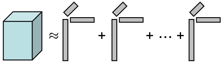
Figure 4: Illustration of the tensor CP model.

3.2 CP Scoring using a Heuristic

We make use of the components extracted by the CP model to assign scores to each pair $(i,j)$ according to their likelihood of linking in the future. The outer product of ${\bm{\mathbf{{a}}}}_{k}$ and ${\bm{\mathbf{{b}}}}_{k}$, i.e., ${\bm{\mathbf{{a}}}}_{k}{\bm{\mathbf{{b}}}}_{k}^{{\sf T}}$, quantifies the relationship between object pairs in component $k$. The temporal profiles are captured in the vectors ${\bm{\mathbf{{c}}}}_{k}$. Different components may have different trends, e.g., they may have increasing, decreasing, or steady profiles. In our heuristic approach, we assume that average activity in the last $T_{0}=3$ years is a good choice for the weight. We define the similarity score for objects $i$ and $j$ using a $K$-component CP model in (14) as the $(i,j)$ entry of the following matrix:

$${\bm{\mathbf{{S}}}}=\sum_{k=1}^{K}\gamma_{k}\lambda_{k}{\bm{\mathbf{{a}}}}_{k}{\bm{\mathbf{{b}}}}_{k}^{{\sf T}},\quad\text{where}\quad\gamma_{k}=\frac{1}{T_{0}}\sum_{t=T-T_{0}+1}^{T}{\bm{\mathbf{{c}}}}_{k}(t).$$ (15)

This is a simple approach, using temporal information from the last $T_{0}=3$ time steps only. In many cases, the simple heuristic of just averaging the last few time steps works quite well and is sufficient. An alternative that provides a more sophisticated use of time is discussed in the next section.

3.3 CP Scoring using Temporal Forecasting

Alternatively, we can use the temporal profiles computed by CP as a basis for predicting the scores in future time steps. In this work, we use the Holt-Winters forecasting method Chatfield and Yar (1988), which is particularly suitable for time-series data with periodic patterns. This is an automatic method which only requires the data and the expected period (e.g., we use $L=7$ for daily data). As will be shown in §5, the Holt-Winters method is fairly accurate in picking up patterns in time and therefore can be used as a predictive tool. If we are predicting for $L$ time steps in the future (one period), we get a tensor of prediction scores of size $M\times N\times L$. This is computed as

$$\bm{\mathscr{{S}}}=\sum_{k=1}^{K}\lambda_{k}{\bm{\mathbf{{a}}}}_{k}\circ{\bm{\mathbf{{b}}}}_{k}\circ\bm{\gamma}_{k}$$ (16)

where each $\bm{\gamma}_{k}$ is a vector of length $L$ that is the prediction for the next $L$ time steps from the Holt-Winters methods with ${\bm{\mathbf{{c}}}}_{k}$ as input.

For our studies, we implemented the additive Holt-Winters method (as described in Chatfield and Yar (1988)), i.e., Holt’s linear trend model with additive seasonality, which corresponds to an exponential smoothing method with additive trend and additive seasonality. For a review of exponential smoothing methods, see Gardner (2006). An example of forecasting using additive Holt-Winters is shown in Figure 5. The input is shown in blue, and the prediction of the next $L=7$ time steps is shown in red. We show examples in §5 that use the actual CP data as input. Forecasting methods beside the Holt-Winters method have also proven useful in analyzing temporal data Makridakis and Hibon (2000). Work on the applicability of different forecasting methods for link prediction is left for future work.

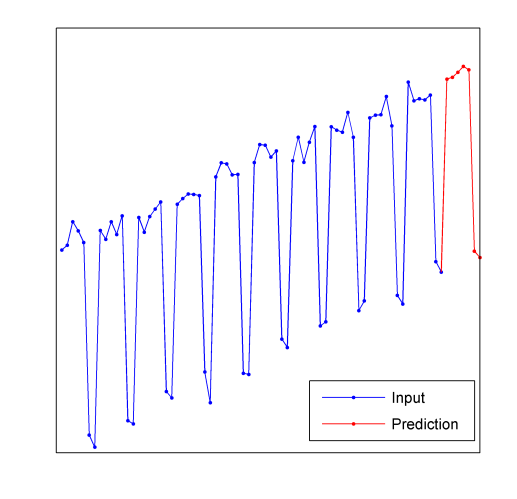
Figure 5: An illustration of the predictions produced by the additive Holt-Winters method on data with a period of $L=7$.

3.4 Computational Complexity and Memory

The computational complexity of CP is $O({\rm nnz}(\bm{\mathscr{{Z}}}))$ per iteration. As with TSVD, we cannot predict the number of iterations in advance. The storage required for CP is $K(M+N+T+1)$, for the three factor matrices and the scalar $\lambda_{k}$ values.

4 Experiments with Link Prediction for One Time Step

We use the DBLP data set to assess the performance of various link predictors discussed in §2 and §3. All experiments were performed using Matlab 7.8 on a Linux Workstation (RedHat 5.2) with 2 Quad-Core Intel Xeon 3.0GHz processors and 32GB RAM. We compute the CP model via an Alternating Least Squares (ALS) approach using the Tensor Toolbox for Matlab Bader and Kolda (2007).

4.1 Data

At the time the DBLP data was downloaded for this work, it contained publications from 1936 through the end of 2007. Here we only consider publications of type inproceedings between 1991 and 2007.

The data is organized as a third-order tensor $\bm{\mathscr{{Z}}}$ of size $M\times N\times T$. We let $\bm{\mathscr{{C}}}(i,j,t)$ denote the total number of papers by author $i$ at conference $j$ in year $t$. In order to decrease the effect of large numbers of publications, we preprocess the data so that

$$\bm{\mathscr{{Z}}}(i,j,t)=\begin{cases}1+\log(\bm{\mathscr{{C}}}(i,j,t))&\text{if }\bm{\mathscr{{C}}}(i,j,t)>0,\\ 0&\text{otherwise}.\end{cases}$$

Using a sliding window approach, we divide the data into seven training/test sets such that each training set contains $T=10$ years and the corresponding test set contains the following 11th year. Table 1 shows the size and density of the training and testing sets. We only keep those authors that have at least 10 publications (i.e., an average of one per year) in the training data, and each test set contains only the authors and conferences available in the corresponding training set.

Training	Test	Authors	Confs.	Training Links	Test Links	Test New Links
Years	Year			(% Density)	(% Density)	(% Density)
1991-2000	2001	7108	1103	112,730 (0.14)	12,596 (0.16)	5,079 (0.06)
1992-2001	2002	8368	1211	134,538 (0.13)	16,115 (0.16)	6,893 (0.07)
1993-2002	2003	9929	1342	162,357 (0.12)	20,261 (0.15)	8,885 (0.07)
1994-2003	2004	11836	1491	196,950 (0.11)	27,398 (0.16)	12,738 (0.07)
1995-2004	2005	14487	1654	245,380 (0.10)	35,089 (0.15)	16,980 (0.07)
1996-2005	2006	17811	1806	308,054 (0.10)	40,237 (0.13)	19,379 (0.06)
1997-2006	2007	21328	1934	377,202 (0.09)	41,300 (0.10)	20,185 (0.05)

Table 1: Training and Test set pairs formed from the DBLP data set.

4.2 Interpretation of CP

Before addressing the link prediction problem, we first discuss how to use the CP model for exploratory analysis of the temporal data. The primary advantage of the CP model is its interpretability, as illustrated in Figure 6, which contains three example components from the 50-component CP model of the tensor representing publications from 1991 to 2000. The factor ${\bm{\mathbf{{a}}}}_{k}$ captures a certain group of authors while ${\bm{\mathbf{{b}}}}_{k}$ extracts the conferences, where the authors captured by ${\bm{\mathbf{{a}}}}_{k}$ publish. Finally, ${\bm{\mathbf{{c}}}}_{k}$ corresponds to the temporal signature, depicting the pattern of the publication history of those authors at those conferences over the associated time period. Therefore, the CP model can address the link prediction problem well by capturing the evolution of the links between objects using the factors in the time mode.

Figure 6a shows the third component with authors (${\bm{\mathbf{{a}}}}_{k}$) in the top plot, conferences (${\bm{\mathbf{{b}}}}_{k}$) in the middle, and time (${\bm{\mathbf{{c}}}}_{k}$) on the bottom. The highest scoring conferences are DAC, ICCAD and ICCD, which are related conferences on computer design. Many authors publish in these conferences between 1991 and 2000, but the top are Vincentelli, Brayton, and others listed in the caption. This author/conference combination has a peak in the early 1990s and starts to decline in mid-’90s. Note that the author and conference scores are mostly positive. Figure 6b shows another example component, which actually has very similar conferences to those in the component discussed above. The leading authors, however, are different. Moreover, the time profile is different with an increasing trend after the mid-’90s. Figure 7 shows a component that detects related conferences that take place only in even years. Again we see that the components are primarily positive. A nice feature of the CP model is that it does not have any constraints (like orthogonality in the SVD) that artificially impose a need for negative entries in the components.

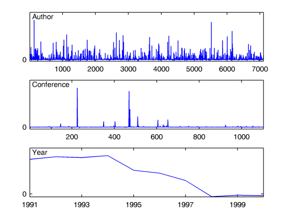
(a) Factors from component 3: Top authors are Alberto L. Sangiovanni Vincentelli, Robert K. Brayton, Sudhakar M. Reddy, and Irith Pomeranz. Top conferences are DAC, ICCAD, and ICCD.

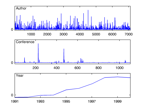
(b) Factors from component 4: Top authors are Miodrag Potkonjak, Massoud Pedram, Jason Cong, and Andrew B. Kahng. Top conferences are DAC, ICCAD, and ASPDAC.

Figure 6: Examples from 50-component CP model of publications from 1991 to 2000.

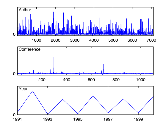
Figure 7: Factors from component 46 of 50-component CP model of publications from 1991 to 2000: Top authors are Franz Baader, Henri Prade, Didier Dubois, and Bernhard Nebel. Top conferences are ECAI and KR.

4.3 Methods and Parameter Selection

The goal of a link predictor in this study is to predict whether the $i$th author is going to publish at the $j$th conference during the test year. Therefore, each nonzero entry in the test set is treated as 1, i.e., a positive link, regardless of the actual number of publications; otherwise, it is 0 indicating that there is no link between the corresponding author-conference pair.

The common parameter for all link predictors, except Katz-CT/CWT, is the number of components, $K$. In our experiments, instead of using a specific value of $K$, which cannot be determined systematically, we use an ensemble approach. Let ${\bm{\mathbf{{S}}}}_{{K}}$ denote the matrix of scores computed for $K=10,20,...100$. Then the matrix of ensemble scores, ${\bm{\mathbf{{S}}}}$, used for link prediction is calculated as

$${\bm{\mathbf{{S}}}}=\sum_{K\in\{10,20,...100\}}\frac{{\bm{\mathbf{{S}}}}_{{K}}}{\left\lVert\,{\bm{\mathbf{{S}}}}_{{K}}\,\right\rVert_{F}}\;.$$

In addition to the number of components, the parameter $\beta$ used in the Katz scores in (12) and (13) needs to be determined. We use $\beta=0.001$, which was chosen such that $\psi^{-}_{p}>0$ for all $p=1,\dots,R$ in (10) for the data in our experiments. We have observed that if $\psi^{-}_{p}<0$ then the scores contain entries with large magnitudes but negative values, which degrades the performance of Katz measure. Finally, $\theta$ is the parameter used for weighting slices while forming the CWT in (2). We set $\theta=0.2$ according to preliminary tests on the training data sets. We use the heuristic scoring method discussed in §3.2 for CP.

4.4 Link Prediction Results

Two experimental set-ups are used to evaluate the performance of the methods.

• Predicting All Links: The first approach compares the methods in terms of how well they predict positive links in the test set.

• Predicting New Links: The second approach addresses a more challenging problem, i.e., how well the methods predict the links that have not been previously seen at any time in the training set.

As an evaluation metric for link prediction performance, we use the area under the receiver operating characteristic curve (AUC) because it is viewed as a robust measure in the presence of imbalance Stager et al. (2006), which is important since less than 0.2% of all possible links exist in our testing data. Figure 8 shows the performance of each link predictor in terms of AUC when predicting all links (blue bars) and new links (red bars). As expected, the AUC values are much lower for the new links. Among all methods, the best performing method in terms of AUC is Katz-CWT. Further, CWT is consistently better on average than the corresponding CT methods, which shows that giving more weight to the data in recent years improves link prediction.

In Figure 9, we show the ROC (receiver operating characteristic) curves; for the purposes of clarity, we omit the CT results. When predicting all links, Figure 9a shows that all methods perform similarly initially, but Katz-CWT is best as the false positive rate increases. TKatz-CWT and TSVD-CWT are only slightly worse than Katz-CWT. Finally, CP starts having false-positives earlier than the other methods. Figure 9b shows the behavior for just the new links. In this case, the relative performance of the algorithms is mostly unchanged.

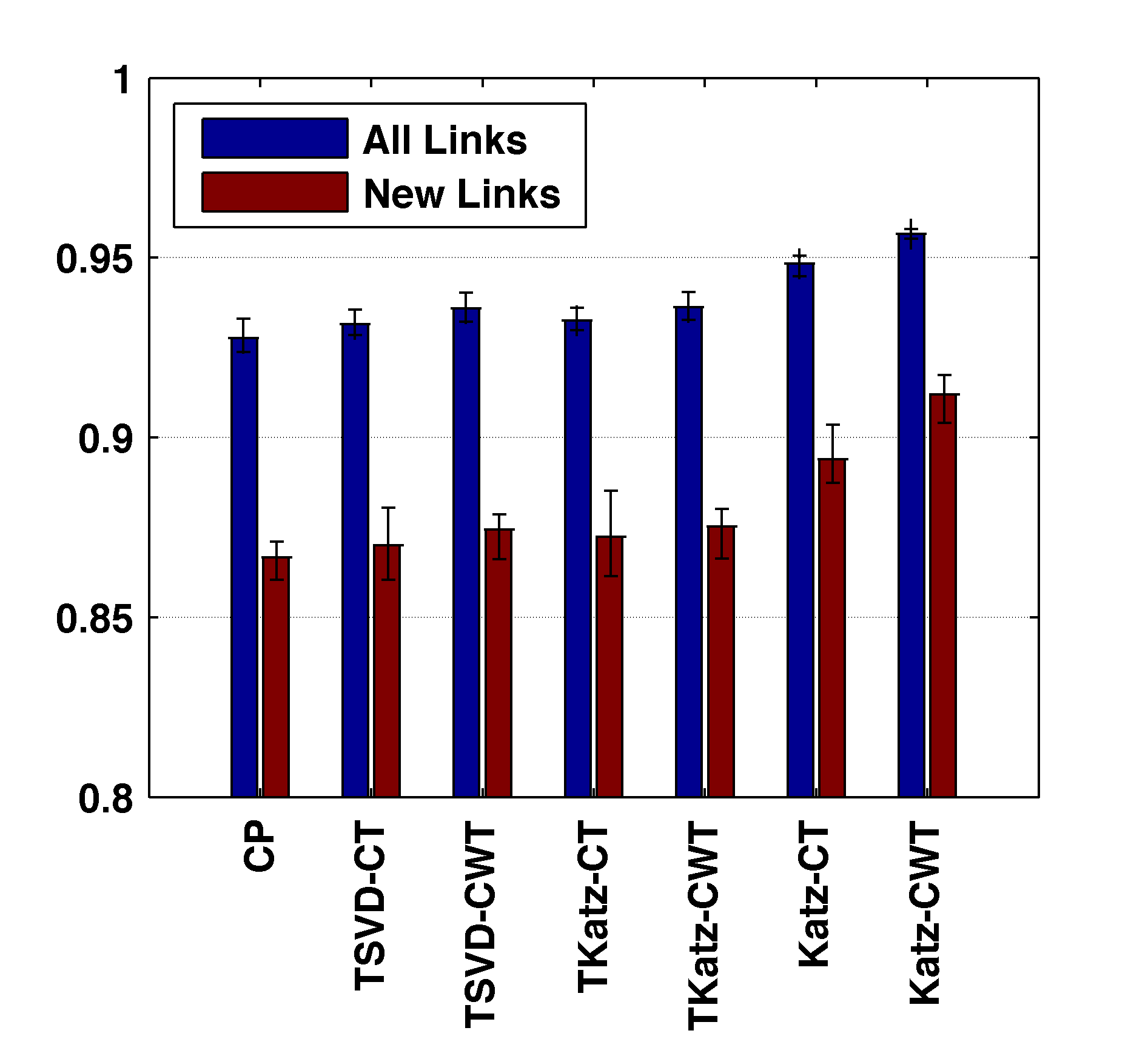
Figure 8: Average link prediction performance of each method across all seven training/test set pairs (black bars show absolute range).

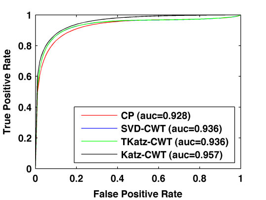
(a) Prediction of all links in the test sets.

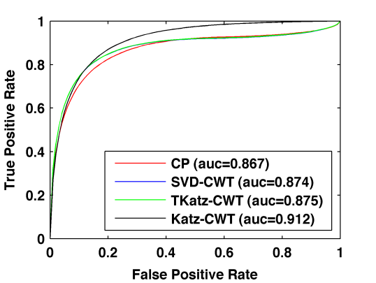
(b) Prediction of new links in the test sets.

Figure 9: Average ROC curves showing the performance of link prediction methods across all training/test sets.

In order to understand the behavior of different link predictors better, we also compute how many correct links (true positives) are in the top 1000 scores predicted by each method. Table 2 shows that CP, TSVD-CWT, TKatz-CWT and Katz-CWT achieve close to 75% accuracy over all links. The accuracy of the methods goes down to 10% or less when we remove all previously seen links from the test set, but this is still very significant. Although 10% accuracy may seem low, this is still two orders of magnitude better than what would be expected by chance (0.1%) due to high imbalance in the data (see the last column of Table 1). Note that the best methods in terms of AUC, i.e., Katz-CT and Katz-CWT, perform worse than CP, TSVD-CWT and TKatz-CWT for predicting new links. We also observe that CP is among the best methods when we look at the top predictions even if it starts giving false-positives earlier than other methods.

Test	CP	TSVD	TSVD	TKatz	TKatz	Katz	Katz
Year		-CT	-CWT	-CT	-CWT	-CT	-CWT
All Links
$2001$	671	617	685	617	686	625	709
$2002$	668	660	674	659	674	658	716
$2003$	723	697	743	693	745	715	754
$2004$	783	726	777	721	776	719	774
$2005$	755	716	776	720	775	700	781
$2006$	807	729	801	731	800	698	796
$2007$	721	681	755	687	754	647	724
Mean	733	689	744	690	744	680	750
New Links
$2001$	87	80	104	80	104	51	56
$2002$	97	84	124	84	124	74	81
$2003$	78	80	96	75	97	55	62
$2004$	99	79	105	81	105	57	69
$2005$	116	89	117	88	117	58	69
$2006$	91	77	110	77	109	63	70
$2007$	83	71	95	73	99	43	42
Mean	93	80	107	80	107	57	64

(a)

Table 2: Correct predictions in top 1000 scores.

The matrix-based methods (TSVD, TKatz and Katz) are quite fast relative to the CP method. Average timings across all training sets are TSVD-CT/CWT and TKatz-CT/CWT: 61 sec.; Katz-CT: 80 sec.; Katz-CWT: 74 sec.; and CP: 1300 sec. Note that for all but the Katz method, the times reflect the computation of models using ranks of $K=10,20,...100$. For the Katz method, a full SVD decomposition is computed, thus making the method too computationally expensive for very large problems.

5 Experiments with Link Prediction for Multiple Time Steps

As might be evident from Figures 6 and 7, the utility of tensor models is in their ability to reveal patterns in time. In this section, we use synthesized data to explore the ramifications of temporal predictions in situations where there are several different periodic patterns in the data. In particular, Figure 7 shows an every other year pattern in the data, but this is not exploited in the predictions in the last section based on the heuristic score in (15). In the DBLP data set, periodic time profiles were few and did not have noticeable impact on performance. Here we simulate the type of data where bringing the time pattern information into play is crucial for predictions. Our goal is to use the periodic information, predicting even further out in time. For example, if we assume that our training data is for times $t=1,\dots,T$ and that the period in our data is of length $L$, then we can predict connections for time periods $T+1$ through $T+L$. In this section, we present results of experiments involving link prediction for multiple time steps. All experiments were performed using Matlab 7.9 on a Linux Workstation (RedHat 5.2) with 2 Quad-Core Intel Xeon 3.0GHz processors and 32GB RAM.

5.1 Data

We generate simulated data that shows connections between two sets of entities over time. In the DBLP data, the entity sets were authors and conferences and each time $t=1,\dots,T$ corresponded to one year of data. In our simulated example, we assume that each time $t$ corresponds to one day and that the temporal profiles correspond roughly to a seven-day period ($L=7$). We might assume that the entities are users and services. For example, most major service providers (Yahoo, Google, MSN, etc.) have a front page. We may wish to predict which users will likely be connecting to which services over time. For example, it may be that there are groups of people that check the National, World, and Business News on weekdays; another group that checks Entertainment Listings on weekends; a group that checks Sports Scores on Mondays; another group uses the service for email every day, etc. Each of these groupings of users and services along with corresponding temporal profile can be represented by a single component in the tensor model. The motivation for link prediction are many-fold. We might want to characterize the temporal patterns so that we know how often to update the services or when to schedule down time. We may use prediction to cache certain data, to better direct advertisements to users, etc. In addition to the business model/motivation, we could also consider the application of cybersecurity using analysis of network traffic data. In this case, the goal is to determine which computers are most likely to contact which other computers. Predicted links could be used to find anomalous or malicious behavior, proactively load balance, etc. In all of these applications, accurately predicting links over multiple time steps is crucial.

We assume that our data can be modeled by $K=10$ components and generate our training and testing tensors as follows.

1. Matrices ${\bm{\mathbf{{A}}}}$ and ${\bm{\mathbf{{B}}}}$ of size $M\times K$ and $N\times K$ are “entity participation” matrices. In other words, column ${\bm{\mathbf{{a}}}}_{k}$ (resp. ${\bm{\mathbf{{b}}}}_{k}$) is the vector of participation levels of all the entities in component $k$. In our tests, we use $M=500$ and $N=400$. Each row is generated by choosing between 1 and $K$ components for the entity to participate in where the probability of participating in at least $k+1$ components is $1-4^{k}$. An example of the distribution of participation is shown in Figure 10; note that most entities participate in just one component. Once the number of components is decided, the specific components that a given entity participates in are chosen uniformly at random. The strength of participation is picked uniformly at random between 1 and 10. Finally, the columns of ${\bm{\mathbf{{A}}}}$ and ${\bm{\mathbf{{B}}}}$ are normalized to length 1.

   

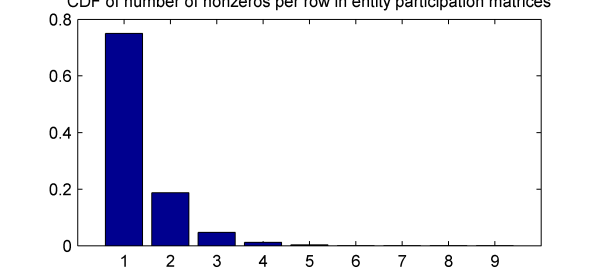
   Figure 10: Example distribution of the number of nonzeros per row in entity participation matrices.

2. In the third mode, the matrix corresponds to time. We assume we have $P$ periods of training data, so that we have $T=LP$ time observations to train on. In our tests, we use $L=7$ and $P=10$. We also assume that we have 1 period of testing data. Therefore, we generate a matrix ${\bm{\mathbf{{C}}}}$ of size $L(P+1)\times K$, which will be divided into submatrices ${\bm{\mathbf{{C}}}}^{\rm[train]}$ and ${\bm{\mathbf{{C}}}}^{\rm[test]}$. Each column of ${\bm{\mathbf{{C}}}}$ is temporal data of length $L(P+1)$ with a repeating period of length $L=7$. We use the periodic patterns shown in Figure 11. For example, the first patten corresponds to a weekday pattern, and the seventh pattern corresponds to Tuesday/Thursday activities. Patterns 1 and 5 are the same but correspond to different sets of entities and so will still be computable in our experiments.

   

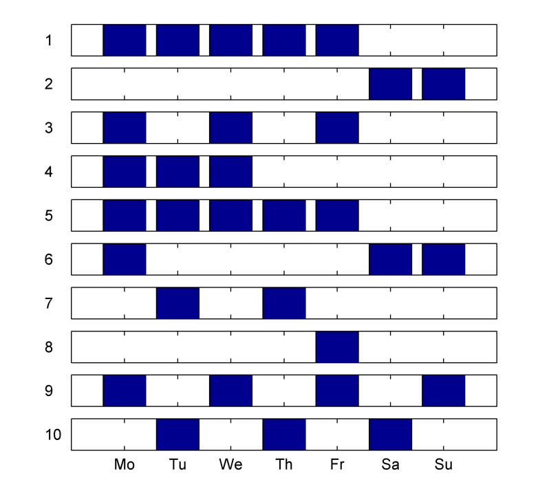
   Figure 11: Weekly patterns of users in simulated data.

   The creation of the temporal data is shown in Figure 12. As shown at the top, in order to generate the temporal data of length $L(P+1)$, we repeat the temporal pattern $P+1$ times. Next, for each of the $K=10$ components, we randomly adjust the data to be increasing, decreasing, or neutral. On the left in the middle plot, we show a decreasing pattern and on the right an increasing pattern. Finally, we add 10% noise, as shown in the lower plots. The final matrix ${\bm{\mathbf{{C}}}}$ is column normalized. The first $T=LP=70$ rows become ${\bm{\mathbf{{C}}}}^{\rm[train]}$ and the last $L=7$ rows become ${\bm{\mathbf{{C}}}}^{\rm[test]}$.

   

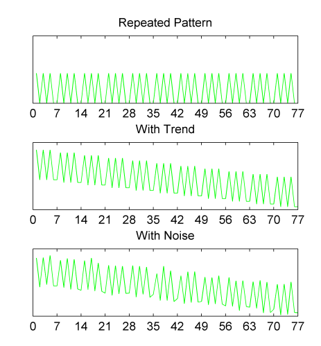
   (a) Pattern 3 and a decreasing trend

   

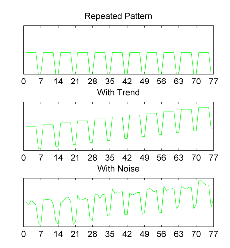
   (b) Pattern 1 and an increasing trend

   Figure 12: Steps to creating the temporal data.

3. We create noise-free versions of the training and testing tensors by computing

   $$\bm{\mathscr{{Z}}}^{\rm[train]}=\sum_{k=1}^{K}{\bm{\mathbf{{a}}}}_{k}\circ{\bm{\mathbf{{b}}}}_{k}\circ{\bm{\mathbf{{c}}}}_{k}^{\rm[train]}\quad\text{and}\quad\bm{\mathscr{{Z}}}^{\rm[test]}=\sum_{k=1}^{K}{\bm{\mathbf{{a}}}}_{k}\circ{\bm{\mathbf{{b}}}}_{k}\circ{\bm{\mathbf{{c}}}}_{k}^{\rm[test]}.$$

   In order to make the problem challenging, we significantly degrade the training data in the next two steps.

4. We take $p_{\rm swap}=50\%$ of the $p_{\rm top}=25\%$ largest entries in $\bm{\mathscr{{Z}}}^{\rm[train]}$ and randomly swap them with other entries in the tensor selected uniformly at random. This has the effect of removing some important data (i.e., large entries) and also adding some spurious data.

5. Finally, we add $p_{\rm rand}=10\%$ percent standard normal noise to every entry of $\bm{\mathscr{{Z}}}^{\rm[train]}$.

For each problem instance, we compute a CP decomposition of $\bm{\mathscr{{Z}}}^{\rm[train]}$ which has had large entries swapped and noise added. Then we use the resulting factorization to predict the largest entries of $\bm{\mathscr{{Z}}}^{\rm[test]}$.

5.2 Methods and Parameter Selection

The goal of this study is to predict the significant entries in $\bm{\mathscr{{Z}}}^{\rm[test]}$. Therefore, without loss of generality, we treat all nonzeros in the test tensor as ones (i.e., positive links) and the rest as zeros (i.e., no link). This results in 15% positives.

We consider the CP model (with $K=10$ components) using the forecasting scoring model described in §3.3. The model parameters for level, trend and seasonality are set to $0.2$ in the Holt-Winters method. We compute the CP model via the CPOPT approach as described in Acar et al. (2009). This is an optimization approach using the nonlinear conjugate gradient method. We set the stopping tolerance on the normalized gradient to be $10^{-8}$, the maximum number of iterations to 1000, and the maximum number of function values to 10,000. The models could have been computed using ALS as in the previous section, but here we use a different technique for variety.

The matrix methods described in §2 are not appropriate for this data because simply collapsing the data will obviously not work. Moreover, there is no clear methodology for predicting out in time. The best we could possibly do would be to construct a matrix model for each day in the week (i.e., one for each $\ell=1,\dots,L$). Such an approach, however, is not parsimonious and would quickly become prohibitive as the number of models grew. Moreover, it would be extremely difficult to assimilate results across the different models for each day.

Therefore, as a comparison, we use the largest values from the most recent period. In MATLAB notation, the predictions are based on $\bm{\mathscr{{Z}}}^{\rm[train]}(:,:,L(P-1)+1:LP)$, i.e., the last $L$ frontal slices of $\bm{\mathscr{{Z}}}^{\rm[train]}$. The highest values in that period are predicted to reappear in the testing period. We call this the Last Period method. Under the scenario considered here, this is an extremely predictive model when the noise levels are low. As we randomly swap data (reflective of random additions and deletions as would be expected in any real world data set), however, the performance of this model degrades.

5.3 Interpretation of CP Results and Temporal Prediction

As mentioned above, we compute the CP factorization of a noisy version of $\bm{\mathscr{{Z}}}^{\rm[train]}$ of size $500\times 400\times 70$. Because the data is noisy (swapping 50% of the 25% largest entries and adding 10% Gaussian noise), the fit of the model to the data is not perfect. In fact, the percentage of the $\bm{\mathscr{{Z}}}^{\rm[train]}$ that is described by the model is only about 50% (averaged over 10 instances).

However, the underlying low-rank structure of the data gives us hope of recovery even in the presence of excessive errors. We can see this in terms of the factor match score (FMS), which is defined as follows. Let the correct and computed factorizations be given by

$$\sum_{k=1}^{K}\lambda_{k}\;{\bm{\mathbf{{a}}}}_{k}\circ{\bm{\mathbf{{b}}}}_{k}\circ{\bm{\mathbf{{c}}}}_{k}\quad\text{and}\quad\sum_{k=1}^{K}\bar{\lambda}_{k}\;{\bm{\bar{}}{\mathbf{{a}}}}_{k}\circ{\bm{\bar{}}{\mathbf{{b}}}}_{k}\circ{\bm{\bar{}}{\mathbf{{c}}}}_{k},$$

respectively. Without loss of generality, we assume that all the vectors have been scaled to unit length and that the scalars are positive. Recall that there is a permutation ambiguity, so all possible matchings of components between the two solutions must be considered. Under these conditions, the FMS is defined as

$$\text{FMS}=\max_{\sigma\in\Pi(K)}\frac{1}{K}\sum_{k=1}^{K}\left(1-\frac{|\lambda_{r}-\bar{\lambda}_{\sigma(k)}|}{\max\{\lambda_{r},\bar{\lambda}_{\sigma(k)}\}}\right)|{\bm{\mathbf{{a}}}}_{k}^{{\sf T}}{\bm{\bar{}}{\mathbf{{a}}}}_{\sigma(k)}||{\bm{\mathbf{{b}}}}_{k}^{{\sf T}}{\bm{\bar{}}{\mathbf{{b}}}}_{\sigma(k)}||{\bm{\mathbf{{c}}}}_{k}^{{\sf T}}{\bm{\bar{}}{\mathbf{{c}}}}_{\sigma(k)}|.$$ (17)

The set $\Pi(K)$ consists of all permutations of 1 to $K$. In our case, we just use a greedy method to determine an appropriate permutation. The FMS can be between 0 and 1, and the best possible FMS is 1. For the problems mentioned above, the FMS scores are around 0.52 on average; yet the predictive power of the CP model is very good (see §5.4).

Figure 13 shows the ten different temporal patterns in the data per the ${\bm{\mathbf{{c}}}}_{k}$ vectors. The green line is the original unaltered data, the first portion of which is used to generate the training data. The blue line is the pattern that is extracted via the CP model. Note that it is generally a good fit to the true data shown in green. Finally, the red line is the prediction generated by the Holt-Winters method using the pattern extracted by CP (i.e., the blue line). The red data corresponds to the $\bm{\gamma}_{k}$ vectors used in (16) for link prediction. The results of the link prediction task are discussed in the next subsection.

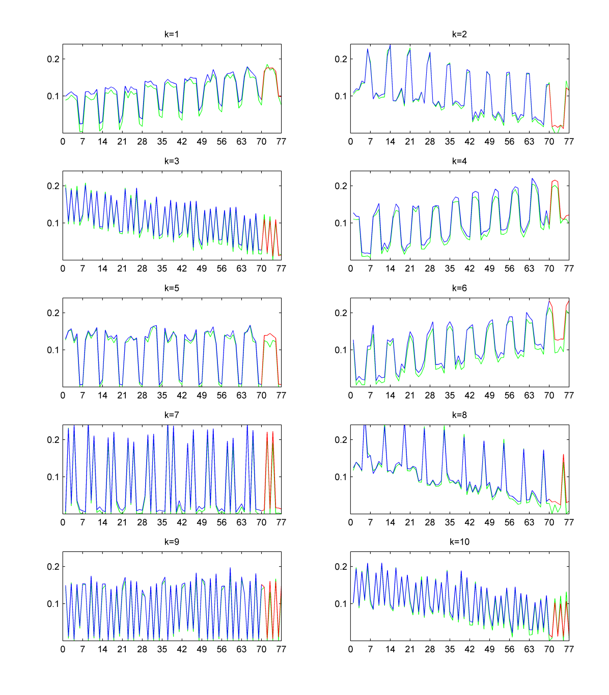
Figure 13: Temporal patterns using Holt-Winters forecasting. The green line is the “true” data. The blue line is the temporal pattern that is computed by CP. The red line is the pattern that is predicted by Holt-Winters using the temporal pattern computed by CP.

5.4 Link Prediction Results

In Figure 14, we present typical ROC curves for the predictions of the next $L=7$ time steps (one period) for a problem instance generated using the procedure mentioned above. As described in §5.2, our goal is to predict the nonzero entries in the testing data $\bm{\mathscr{{Z}}}^{\rm[test]}$ based on the CP model and the score in (16). We compare with the predictions based on the last period in the data. Despite the high level of noise, the CP method is able to get an AUC score of $0.845$, which is much better than then the “Last Period” method’s score of $0.686$. We also considered the accuracy in the first 1,000 values returned. The CP-based method is 100% accurate in its top 1,000 scores whereas the “Last Period” method is only 70% accurate.

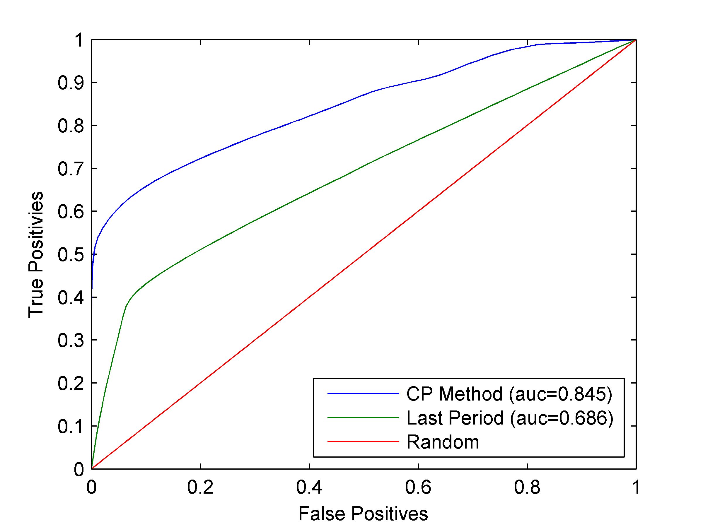
Figure 14: ROC curves and AUC scores for typical problem of predicting links seven steps forward in time.

To investigate the effect of noise on the performance of the CP and Last Period methods, we ran several experiments varying the different amounts of noise ($p_{\rm top}$, $p_{\rm swap}$, and $p_{\rm rand}$). For each experiments, we fixed all but one type of noise, varying the remaining type of noise. The fixed values for each type of noise were the same as those for the experiment described above, while varying $p_{\rm top}$ up to 30%, $p_{\rm swap}$ up to 80%, and $p_{\rm rand}$ up to 40%. For each level of noise, we generated 10 instances of $\bm{\mathscr{{Z}}}^{\rm[train]}$ and $\bm{\mathscr{{Z}}}^{\rm[test]}$ and computed the average AUC and percentage of links correctly predicted in the top 1000 scores.

Figure 15 shows the results of the experiments when varying $p_{\rm swap}$. As expected, AUC values decrease as the number of the most significant links in the training data being swapped randomly is increased. However, there is a clear advantage of the CP method over the Last Period method as depicted in Figure 15a. Note also that in Figure 15b, we see that even as the number of randomly swapped significant links is increased in the training data, the top 1000 scores predicted with the CP method are all correctly identified as links. For the Last Period method, performance decreases as $p_{\rm swap}$ increases, highlighting a clear advantage of the CP method. Figure 16 and Figure 17 present the results for the experiments where $p_{\rm top}$ and $p_{\rm rand}$ were varied, respectively. In both sets of experiments, the CP method consistently performed better than the Last Period method in terms of both AUC and correct predictions in the top 1000 scores for each method. However, no significant changes were detected across the different levels of $p_{\rm top}$ and $p_{\rm rand}$.

The key conclusions from these experiments is that the CP model performs extremely well even when a large percentage of the strongest signals (i.e., link information) in the training data is altered. Such robustness is crucial for applications where noise or missing data is common, e.g., analysis of computer network traffic where data is lost or even hidden in the context of malicious behavior or the analysis of user-service relationships where both user and service profiles are changing over time.

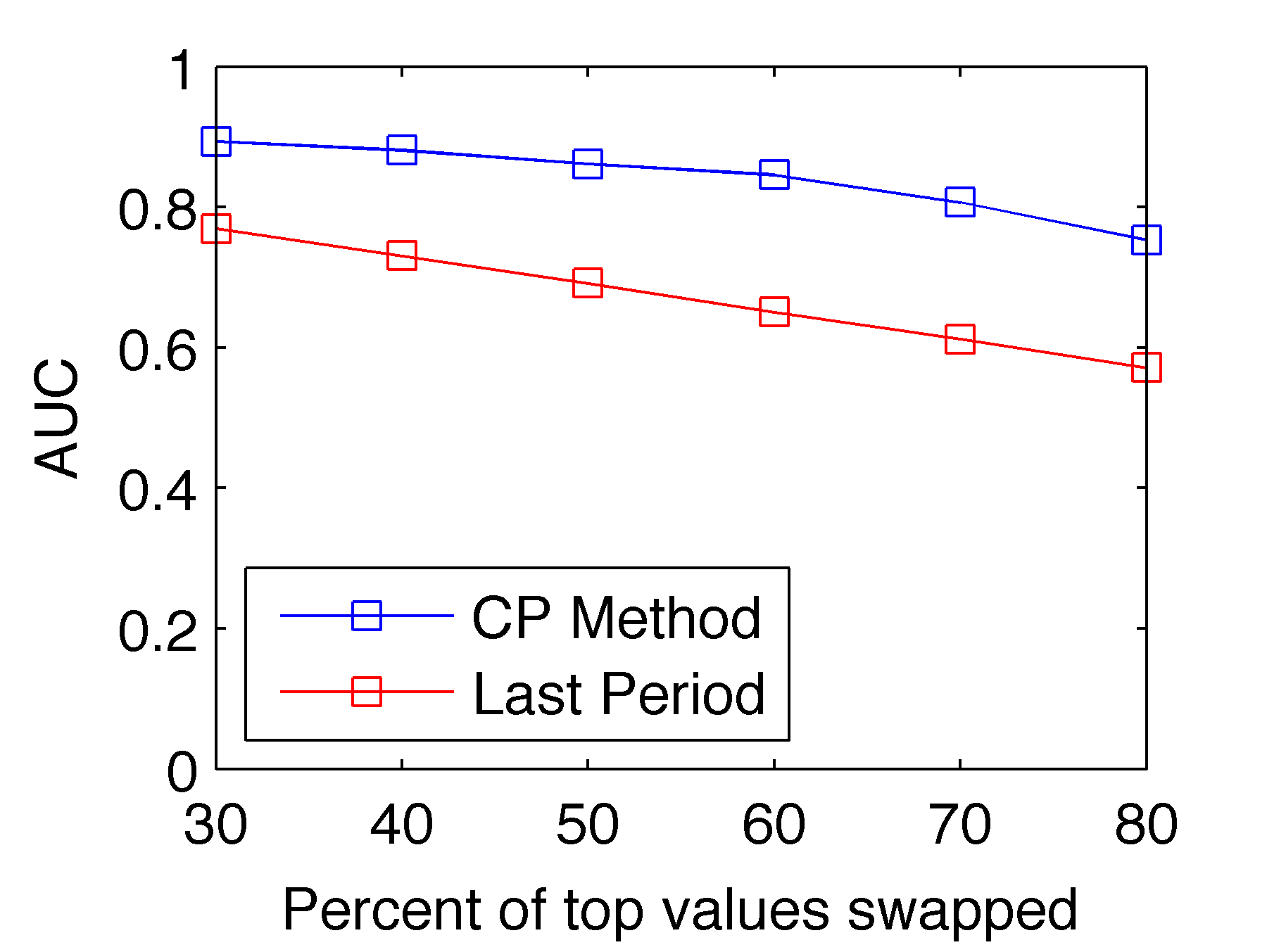
(a) AUC

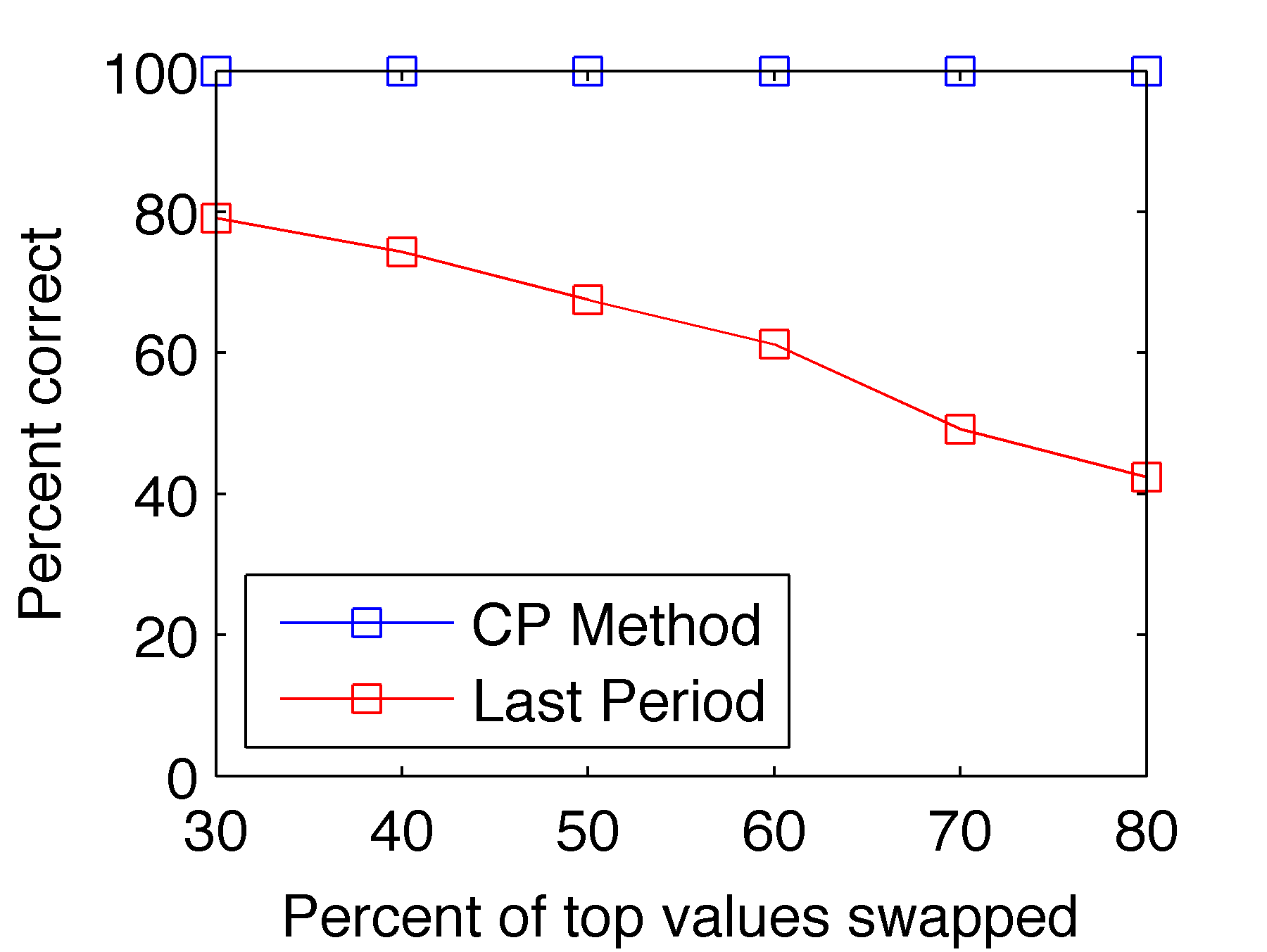
(b) Percent Correct in Top 1000

Figure 15: Impact of varying swapping noise ($p_{\rm swap}$) averaged over 10 runs per noise value.

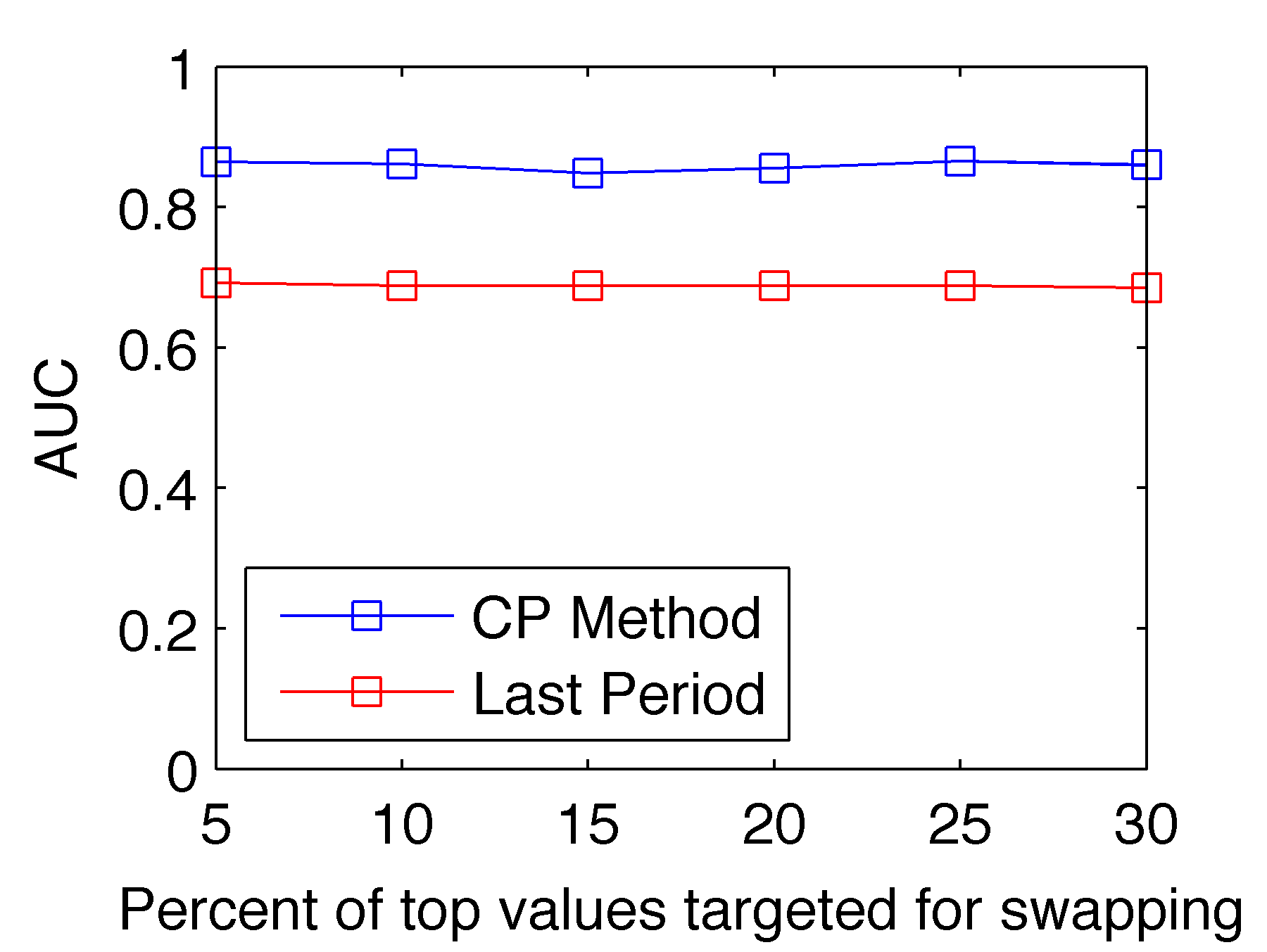
(a) AUC

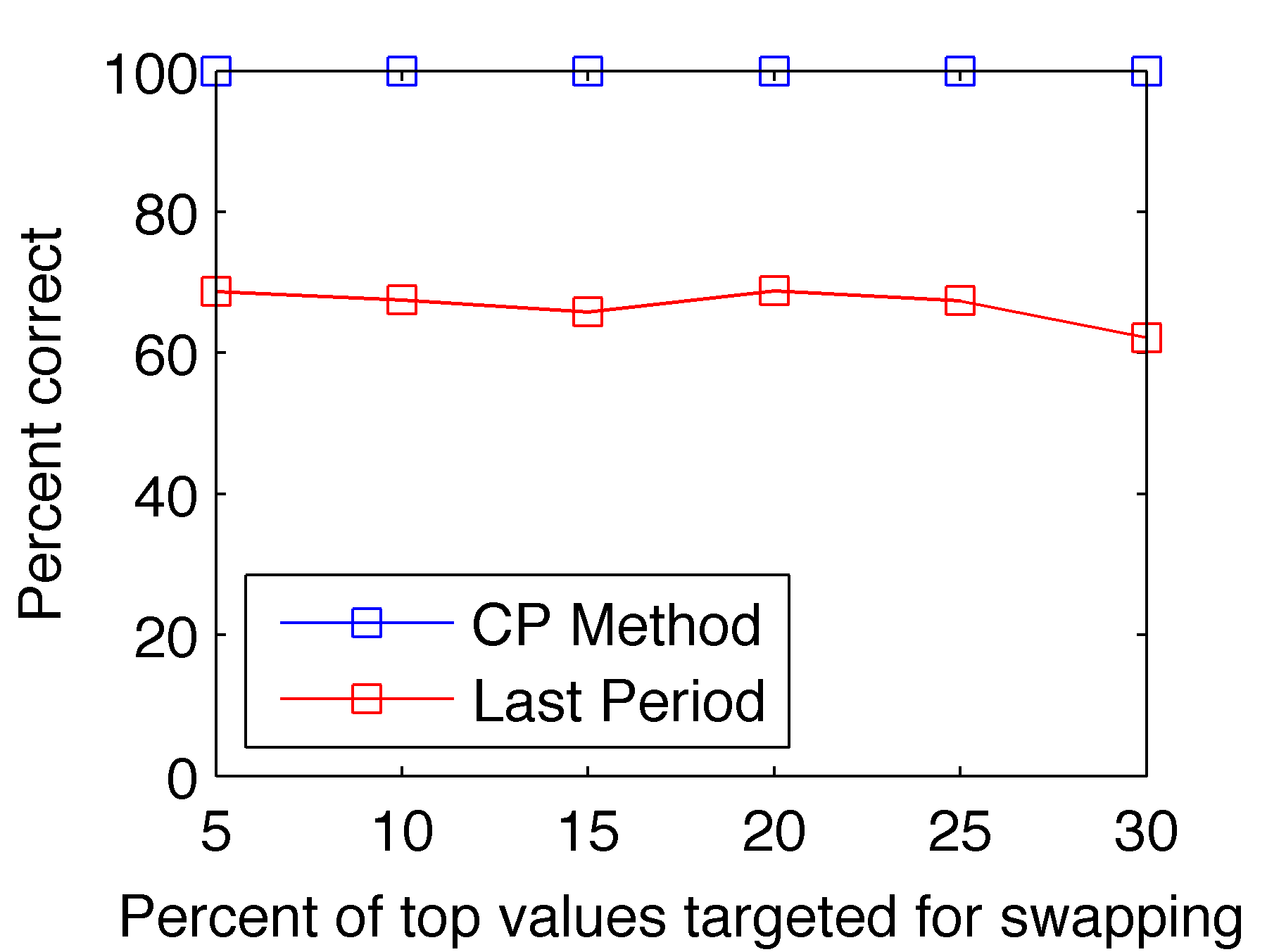
(b) Percent Correct in Top 1000

Figure 16: Impact of varying random noise ($p_{\rm top}$) averaged over 10 runs per noise value.

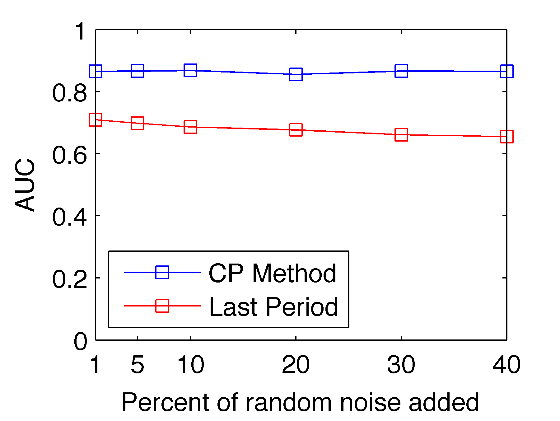
(a) AUC

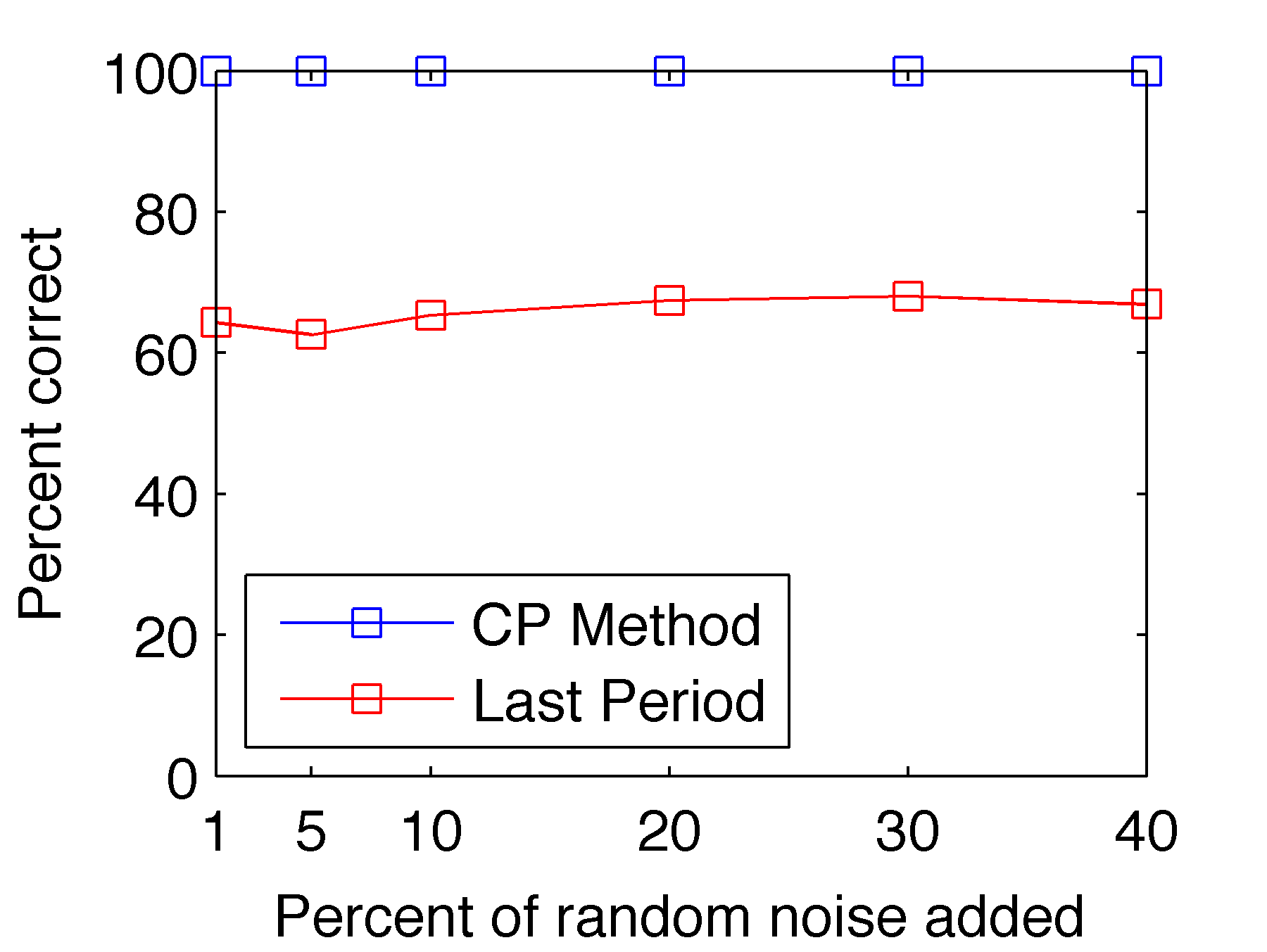
(b) Percent Correct in Top 1000

Figure 17: Impact of varying random noise ($p_{\rm rand}$) averaged over 10 runs per noise value.

Results for different sizes of tensors illustrate that these conclusions hold for larger data sets as well. Figure 18 presents plots of (a) the time required to compute the CP models and Holt-Winters forecasts and (b) the AUC scores for predicting seven steps out in time for tensors of sizes $125\times 100\times 77$, $250\times 200\times 77$, $500\times 400\times 77$ (M=500), $1000\times 800\times 77$ (M=1000), and $2000\times 1600\times 77$. For each size, 10 tensors were generated using the procedures in §5.2, and the box and whiskers plots in Figure 18 present the median (red center mark of boxes), middle quartile (top and bottom box edges), and outlier (red plus marks) summary statistics across the experiments. These results support the conclusions above: predictions using the CP model are more accurate than those computed using the last period to predict an entire period of links.

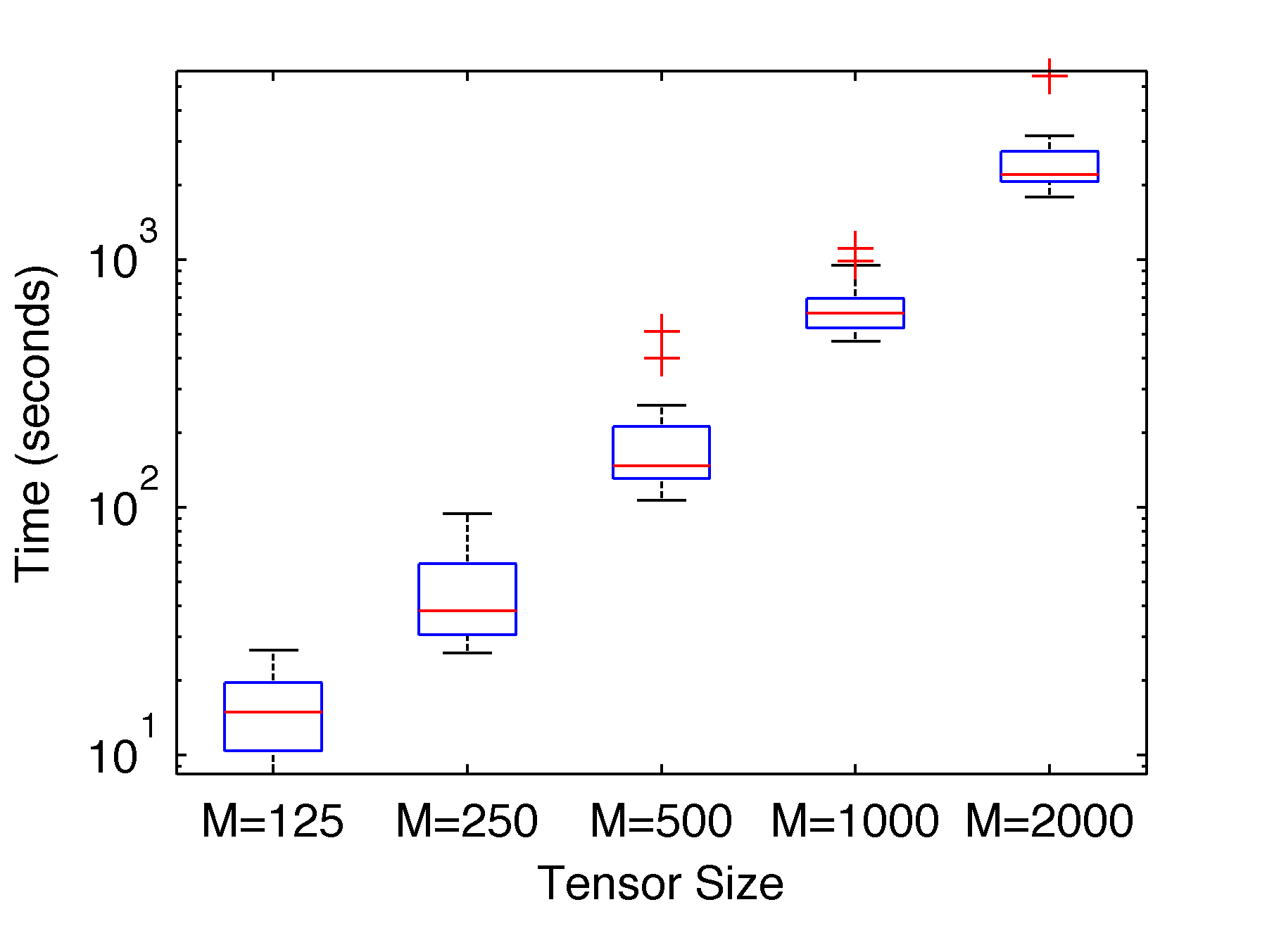
(a) Timings

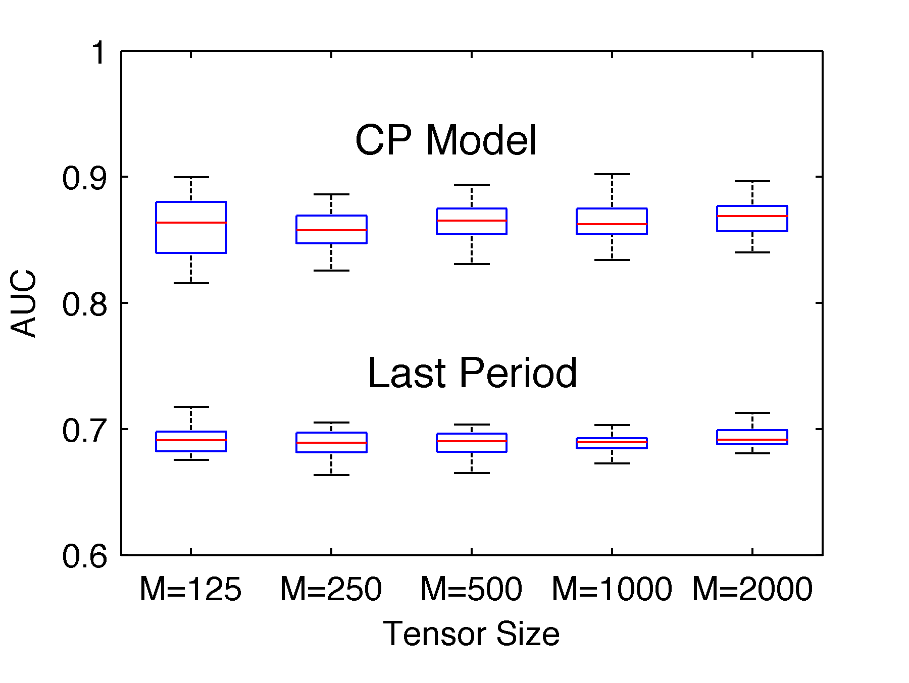
(b) AUC

Figure 18: Results of computing 10 CP models and Holt-Winters forecasts for tensors of different sizes: $125\times 100\times 77$ (M=125); $250\times 200\times 77$ (M=250); $500\times 400\times 77$ (M=500); $1000\times 800\times 77$ (M=1000); $2000\times 1600\times 77$ (M=2000). Computation wall clock times in seconds are shown in (a) and AUC scores are shown in (b).

6 Related Work

Getoor and Diehl 2005 present a survey of link mining tasks, including node classification, group detection, and numerous other tasks including link prediction. Sharan and Neville 2008 consider the goal of node classification for temporal-relational data, suggesting the idea of a “summary graph” of weighted snapshots in time which we have incorporated into this work.

The seminal work of Liben-Nowell and Kleinberg 2007 examines numerous methods for link prediction on co-authorship networks in arXiv bibliometric data. However, temporal information was unused (e.g., as in Sharan and Neville (2008)) except for splitting the data. The proportion of new links ranged from 0.1–0.5% and is thus comparable to what we see in our data (0.05–0.07%). According to Liben-Nowell and Kleinberg, Katz and its variants are among the best link predictors; this observation has been supported by other work as well Huang et al. (2005); Wang et al. (2007). We note that Wang, Satuluri and Parthasarathy 2007 use the truncated sum approximate Katz measure discussed in §2.3 and recommend AUC as one evaluation measure for link prediction because it does not require any arbitrary cut-off. Rattigan and Jensen 2005 contend that the link mining problem is too difficult, in part because the proportion of actual links is very small compared to the number of possible links; specifically, they consider co-author relationships in DBLP data and observe that the proportion of new links is less than 0.01%. (Although we also use DBLP data, we consider author-conference links which has 0.05% or more new links.)

Another way to approach link prediction is to treat it as a straightforward classification problem by computing features for possible links and using a state-of-the-art classification engine like support vector machines. Al Hasan et al. 2006 use this approach in the task of author-author link prediction. They randomly pick equal sized sets of linked and unlinked pairs of authors. They compute features such as keyword similarity, neighbor similarity, shortest path, etc. However, it would likely be computationally intractable to use such a method for computing all possible links due to the size of the problem and imbalance between linked and unlinked pairs of authors. Clauset, Moore, and Newman 2008 predict links (or anomalies) using Monte-Carlo sampling on all possible dendrogram models of a graph. Smola and Kondor 2003 identify connections between link prediction methods and diffusion kernels on graphs but provide no numerical experiments to support this.

Modeling the time evolution of graphs has been considered, e.g., by Sakar et al. 2007 who create time-evolving co-occurrence models that map entities into an evolving latent space. Tong et al. 2008 also compute centrality measures on time evolving bipartite graphs by aggregating adjacency matrices over time in similar approaches to those in §2.1.

Link prediction is also related to the task of collaborative filtering. In the Netflix contest, for example, Bell and Koren 2007 consider the “binary view of the data” as important as the ratings themselves. In other words, it is important to first predict who is likely to rate what before focusing on the ratings. This was a specific task in KDD Cup 2007 Liu and Kou (2007). More recent models by Koren Koren (2009) explicitly account for changes in user preferences over time. And Xiong et al. 2010 propose a probabilistic tensor factorization to address the problem of collaborative filtering over time.

Tensor factorizations have been previously applied in web link analysis Kolda et al. (2005) and also in social networks for the analysis of chatroom Acar et al. (2006) and email communications Bader et al. (2007); Sun et al. (2009). In these applications tensor factorizations are used as exploratory analysis tools and do not address the link prediction problem.

7 Conclusions

In this paper, we explore several matrix- and tensor-based approaches to solving the link prediction problem. We consider author-conference relationships in bibliometric data and a simulation indicative of user-service relationships in an online context as example applications, but the methods presented here also have applications in other domains such as predicting Internet traffic, flight reservations, and more. For the matrix methods, our results indicate that using a temporal model to combine multiple time slices into a single training matrix is superior to simple summation of all temporal data. We also show how to extend Katz to bipartite graphs (e.g., for analyzing relationships between two different types of nodes) and to efficiently compute an approximation to Katz based on the truncated SVD. However, none of the matrix-based methods fully leverages and exposes the temporal signatures in the data. We present an alternative: the CP tensor factorizations. Temporal information can be incorporated into the CP tensor-based link prediction analysis to gain a perspective not available when computing using matrix-based approaches.

We have considered these methods in terms of their AUC scores and the number of correct predictions in the top scores. In both cases, we can see that all the methods do quite well on the DBLP data set. Katz has the best AUC but is not computationally tractable for large-scale problems; however, the other methods are not far behind. Moreover, TKatz-CWT is best for predicting new links in the DBLP data. Our numerical results also show that the tensor-based methods are competitive with the matrix-based methods in terms of link prediction performance.

The advantage of tensor-based methods is that they can better capture and exploit temporal patterns. This is illustrated in the user-service example. In this case, we accurately predicted links several days out even though the underlying dynamics of the process was much more complicated than in the DBLP case.

The current drawback of the tensor-based approach is that there is typically a higher computational cost incurred, but the software for these methods is quite new and will no doubt be improved in the near future.

References

- Acar et al. (2006) Acar, E., Çamtepe, S. A., and Yener, B. 2006. Collective sampling and analysis of high order tensors for chatroom communications. In ISI 2006: Proceedings of the IEEE International Conference on Intelligence and Security Informatics. Lecture Notes in Computer Science, vol. 3975. Springer, Berlin / Heidelberg, 213–224.
- Acar et al. (2009) Acar, E., Kolda, T. G., and Dunlavy, D. M. 2009. An optimization approach for fitting canonical tensor decompositions. Tech. Rep. SAND2009-0857, Sandia National Laboratories, Albuquerque, New Mexico and Livermore, California. Feb. Submitted for publication.
- Acar and Yener (2009) Acar, E. and Yener, B. 2009. Unsupervised multiway data analysis: A literature survey. IEEE Transactions on Knowledge and Data Engineering 21, 1 (Jan.), 6–20.
- Bader et al. (2007) Bader, B. W., Berry, M. W., and Browne, M. 2007. Discussion tracking in Enron email using PARAFAC. In Survey of Text Mining: Clustering, Classification, and Retrieval, Second Edition, M. W. Berry and M. Castellanos, Eds. Springer, 147–162.
- Bader and Kolda (2007) Bader, B. W. and Kolda, T. G. 2007. Efficient MATLAB computations with sparse and factored tensors. SIAM Journal on Scientific Computing 30, 1 (Dec.), 205–231.
- Bast and Majumdar (2005) Bast, H. and Majumdar, D. 2005. Why spectral retrieval works. In SIGIR ’05: Proceedings of the 28th annual international ACM SIGIR conference on Research and development in information retrieval. 11–18.
- Bell and Koren (2007) Bell, R. M. and Koren, Y. 2007. Lessons from the Netflix Prize Challenge. ACM SIGKDD Explorations Newsletter 9, 75–79.
- Carroll and Chang (1970) Carroll, J. D. and Chang, J. J. 1970. Analysis of individual differences in multidimensional scaling via an N-way generalization of “Eckart-Young” decomposition. Psychometrika 35, 283–319.
- Chatfield and Yar (1988) Chatfield, C. and Yar, M. 1988. Holt-winters forecasting: Some practical issues. Journal of the Royal Statistical Society. Series D (The Statistician) 37, 2, 129–140.
- Clauset et al. (2008) Clauset, A., Moore, C., and Newman, M. 2008. Hierarchical structure and the prediction of missing links in networks. Nature 453.
- Dumais et al. (1988) Dumais, S. T., Furnas, G. W., Landauer, T. K., Deerwester, S., and Harshman, R. 1988. Using latent semantic analysis to improve access to textual information. In CHI ’88: Proceedings of the SIGCHI Conference on Human Factors in Computing Systems. ACM Press, 281–285.
- Gardner (2006) Gardner, E. S. 2006. Exponential smoothing: The state of the art - part ii. International Journal of Forecasting 22, 637–666.
- Getoor and Diehl (2005) Getoor, L. and Diehl, C. P. 2005. Link mining: a survey. ACM SIGKDD Explorations Newsletter 7, 2, 3–12.
- Harshman (1970) Harshman, R. A. 1970. Foundations of the PARAFAC procedure: Models and conditions for an “explanatory” multi-modal factor analysis. UCLA working papers in phonetics 16, 1–84. Available at http://www.psychology.uwo.ca/faculty/harshman/wpppfac0.pdf.
- Hasan et al. (2006) Hasan, M. A., Chaoji, V., Salem, S., and Zaki, M. 2006. Link prediction using supervised learning. In Proc. SIAM Data Mining Workshop on Link Analysis, Counterterrorism, and Security.
- Huang et al. (2005) Huang, Z., Li, X., and Chen, H. 2005. Link prediction approach to collaborative filtering. In JCDL ’05: Proc. of the 5th ACM/IEEE-CS joint conference on Digital libraries. 141–142.
- Huang and Lin (2009) Huang, Z. and Lin, D. K. J. 2009. The time-series link prediction problem with applications in communication surveillance. INFORMS Journal on Computing 21, 286–303.
- Katz (1953) Katz, L. 1953. A new status index derived from sociometric analysis. Psychometrika 18, 1 (Mar.), 39–43.
- Kolda and Bader (2009) Kolda, T. G. and Bader, B. W. 2009. Tensor decompositions and applications. SIAM Review 51, 3 (Sept.), 455–500.
- Kolda et al. (2005) Kolda, T. G., Bader, B. W., and Kenny, J. P. 2005. Higher-order web link analysis using multilinear algebra. In ICDM 2005: Proceedings of the 5th IEEE International Conference on Data Mining. IEEE Computer Society, 242–249.
- Koren (2009) Koren, Y. 2009. Collaborative filtering with temporal dynamics. In KDD ’09: Proceedings of the 15th ACM SIGKDD international conference on Knowledge discovery and data mining. ACM, New York, NY, USA, 447–456.
- Koren et al. (2009) Koren, Y., Bell, R., and Volinsky, C. 2009. Matrix factorization techniques for recommender systems. IEEE Computer 42, 30–37.
- Kruskal (1989) Kruskal, J. B. 1989. Rank, decomposition, and uniqueness for 3-way and -way arrays. In Multiway Data Analysis, R. Coppi and S. Bolasco, Eds. North-Holland, Amsterdam, 7–18.
- Liben-Nowell and Kleinberg (2007) Liben-Nowell, D. and Kleinberg, J. 2007. The link-prediction problem for social networks. Journal of the American Society for Information Science and Technology 58, 7, 1019–1031.
- Liu and Kou (2007) Liu, Y. and Kou, Z. 2007. Predicting who rated what in large-scale datasets. ACM SIGKDD Explorations Newsletter 9, 62–65.
- Makridakis and Hibon (2000) Makridakis, S. and Hibon, M. 2000. The m3 competition: results, conclusions and implications. International Journal of Forecasting 16, 451–476.
- Rattigan and Jensen (2005) Rattigan, M. J. and Jensen, D. 2005. The case for anomalous link discovery. ACM SIGKDD Explorations Newsletter 7, 2, 41–47.
- Saad (1992) Saad, Y. 1992. Numerical Methods for Large Eigenvalue Problems. Manchester University Press.
- Sarkar et al. (2007) Sarkar, P., Siddiqi, S. M., and Gordon, G. J. 2007. A latent space approach to dynamic embedding of co-occurrence data. In AI-STATS’07: Proceedings of the Eleventh International Conference on Artificial Intelligence and Statistics (electronic).
- Sharan and Neville (2008) Sharan, U. and Neville, J. 2008. Temporal-relational classifiers for prediction in evolving domains. In ICDM ’08: Proceedings of the 2008 Eighth IEEE International Conference on Data Mining. IEEE Computer Society, 540–549.
- Smola and Kondor (2003) Smola, A. and Kondor, R. 2003. Kernels and regularization on graphs. In Proceedings of the Annual Conference on Computational Learning Theory and Kernel Workshop, B. Schölkopf and M. Warmuth, Eds. Lecture Notes in Computer Science. Springer.
- Stager et al. (2006) Stager, M., Lukowicz, P., and Troster, G. 2006. Dealing with class skew in context recognition. In ICDCSW’06: Proceedings of the 26th IEEE International Conference on Distributed Computing Systems Workshops. 58.
- Sun et al. (2009) Sun, J., Papadimitriou, S., Lin, C.-Y., Cao, N., Liu, S., and Qian, W. 2009. Multivis: Content-based social network exploration through multi-way visual analysis. In SDM’09: Proceedings of the Ninth SIAM International Conference on Data Mining. 1064–1075.
- Tong et al. (2008) Tong, H., Papadimitriou, S., Yu, P. S., and Faloutsos, C. 2008. Proximity tracking on time-evolving bipartite graphs. In SDM’08: Proceedings of the Eighth SIAM International Conference on Data Mining. 704–715.
- Tucker (1963) Tucker, L. R. 1963. Implications of factor analysis of three-way matrices for measurement of change. In Problems in Measuring Change, C. W. Harris, Ed. University of Wisconsin Press, 122–137.
- Tucker (1966) Tucker, L. R. 1966. Some mathematical notes on three-mode factor analysis. Psychometrika 31, 279–311.
- Wang et al. (2007) Wang, C., Satuluri, V., and Parthasarathy, S. 2007. Local probabilistic models for link prediction. In ICDM’07: Proc. of the Seventh IEEE Conference on Data Mining. 322–331.
- Xiong et al. (2010) Xiong, L., Chen, X., Huang, T.-K., Schneider, J., and Carbonell, J. G. 2010. Temporal collaborative filtering with bayesian probabilistic tensor factorization.
- Yan et al. (2008) Yan, H., Grosky, W. I., and Fotouhi, F. 2008. Augmenting the power of LSI in text retrieval: Singular value rescaling. Data & Knowledge Engineering 65, 108–125.