Implicit particle filters for data assimilation

Abstract

Implicit particle filters for data assimilation update the particles by first choosing probabilities and then looking for particle locations that assume them, guiding the particles one by one to the high probability domain. We provide a detailed description of these filters, with illustrative examples, together with new, more general, methods for solving the algebraic equations and with a new algorithm for parameter identification.

1 Introduction

There are many problems in science, for example in meteorology and economics, in which the state of a system must be identified from an uncertain equation supplemented by noisy data (see e.g. [7, 15]). A natural model of this situation consists of an Ito stochastic differential equation (SDE):

$$dx=f(x,t)\,dt+g(x,t)\,dw,$$ (1)

where $x=(x_{1},x_{2},\dots,x_{m})$ is an $m$-dimensional vector, $f$ is an $m$-dimensional vector function, $g(x,t)$ is an $m$ by $m$ matrix, and $w$ is Brownian motion which encapsulates all the uncertainty in the model. In the present paper we assume for simplicity that the matrix $g(x,t)$ is diagonal. The initial state $x(0)$ is given and may be random as well.

The SDE is supplemented by measurements $b^{n}$ at times $t^{n},n=0,1,\dots$. The measurements are related to the state $x(t)$ by

$$b^{n}=h(x^{n})+GW^{n},$$ (2)

where $h$ is a $k$-dimensional, generally nonlinear, vector function with $k\leq m$, $G$ is a matrix, $x^{n}=x(t^{n})$, and $W^{n}$ is a vector whose components are independent Gaussian variables of mean 0 and variance 1, independent also of the Brownian motion in equation (1). The independence requirements can be greatly relaxed but will be observed in the present paper. The task of a filter is to assimilate the data, i.e., estimate $x$ on the basis of both equation (1) and the observations (2).

If the system (1) and equation (2) are linear and the data are Gaussian, the solution can be found in principle via the Kalman-Bucy filter (see e.g. [12]). In the general case, one often estimates $x$ as a statistic (often the mean) of a probability density function (pdf) evolving under the combined effect of equations (1) and (2). The initial state $x^{0}$ being known, all one has to do is evaluate sequentially the pdfs $P_{n+1}$ of the variables $x^{n+1}$ given the equations and the data. In a “particle” filter this is done by following “particles” (replicas of the system) whose empirical distribution at time $t^{n}$ approximates $P_{n}$. One may for example (see e.g. [1, 7, 8, 12]) use the pdf $P_{n}$ and equation (1) to generate a prior density (in the sense of Bayes) , and then use the data $b^{n+1}$ to generate sampling weights which define a posterior density $P_{n+1}$. In addition, one has to sample backward to take into account the information each measurement provides about the past. This process can be very expensive because in most weighting schemes, most of the weights tend to zero fast and the number of particles needed can grow catastrophically (see e.g. [14, 2]); various strategies have been proposed to ameliorate this problem.

Our remedy is implicit sampling [5, 6]. The number of particles needed in a filter remains moderate if one can find high probability particles; to this end, implicit sampling works by first picking probabilities and then looking for particles that assume them, so that particles are guided efficiently to the high probability region one at a time, without needing a global guess of the target density. In the present paper we provide an expository account of particle filters, separating clearly the general principles from details of implementation; we provide general solution algorithms for the resulting algebraic equations, in particular for nonconvex cases which we had not considered in our previous publications, as well as a new algorithm for parameter identification based on an implicit filter. We also provide examples, in particular of nonconvex problems.

Implicit filters are a special case of chainless/Markov field sampling methods [3, 4]; a key connection was made in [16, 17], where it was observed that in the sampling of stochastic differential equations, the marginals needed in Markov field sampling can be read off the equations and need not be estimated numerically.

2 The mathematical framework

The conditional probability density $P_{n}(x)$ at time $t^{n}$, determined by the SDE (1) given the observations (2), satisfies the recurrence relation (see e.g. [7]):

$$P_{n+1}(x^{n+1})=P_{n}(x^{n})P(x^{n+1}|x^{n})P(b^{n+1}|x^{n+1})/Z_{0},$$ (3)

where $P_{n+1}(x^{n+1})$ is the probability of the sample $x^{n+1}$ at time $t^{n+1}$ given the observations $b^{j}$ for $j\leq{n+1}$, $P_{n}(x^{n})$ is the probability of a the sample $x^{n}$ at time $t^{n}$ given the observations $b^{j}$ for $j\leq n$, $P({x}^{n+1}|x^{n})$ is the probability of a sample $x^{n+1}$ at time $t^{n+1}$ given a sample $x^{n}$ at time $t^{n}$, $P(b^{n+1}|x^{n+1})$ is the probability of the observations $b^{n+1}$ given the sample $x^{n+1}$ at time $t^{n+1}$, and $Z_{0}$ is a normalization constant independent of $x^{n}$ and $x^{n+1}$. This is Bayes’ theorem.

We estimate $P_{n+1}$ with the help of M particles, with positions $X_{i}^{n}$ at time $t^{n}$ and $X^{n+1}_{i}$ at time $t^{n+1}$ ($i=1,\dots,M$), which define empirical densities $\hat{P}_{n},\hat{P}_{n+1}$ that approximate $P_{n},P_{n+1}$. We do this by requiring that, when a particle moves from $X_{i}^{n}$ to $X^{n+1}_{i}$ the probability of $X^{n+1}_{i}$ be

$$P(X^{n+1}_{i})=P(X^{n}_{i})P(X^{n+1}_{i}|X^{n}_{i})P(b^{n+1}|X^{n+1}_{i})/Z_{0},$$ (4)

where the hats have been omitted, $P(X^{n}_{i})$, the probability of $X^{n}_{i}$, is assumed given, the pdf $P(X^{n+1}_{i}|X^{n}_{i})$, the probability of $X^{n+1}_{i}$ given $X^{n}_{i}$, is determined by the SDE (1), the pdf $P(b^{n+1}|X^{n+1}_{i})$, the probability of the observations $b^{n+1}$ given the new positions $X^{n+1}_{i}$, is determined by the observation equation (2). We shall see below that one can set $P(X^{n}_{i})=1$ without loss of generality.

Equation (4) defines the pdf we need to sample for each particle; this pdf is known, in the sense that once one has a sample, one can evaluate its probability (up to a constant); the difficulty is to find high probability samples, especially when the number of variables is large. The idea in implicit sampling is to define probabilities first, and then look for particles that assume them; this is done by choosing once and for all a fixed reference random variable, say $\xi$, with a given pdf, say a Gaussian $\exp(-\xi^{T}\xi/2)/(2\pi)^{m/2})$, which one knows how to sample so that most samples have high probability, and then making $X^{n+1}_{i}$ a function of $\xi$, a different function of each particle and each step, each function designed so that the map $\xi\rightarrow X^{n+1}_{i}$ connects highly probable values of $\xi$ to highly probable values of $X^{n+1}_{i}$. To that end, write

$$P(X^{n+1}_{i}|X^{n}_{i})P(b^{n+1}|X^{n+1}_{i})=\exp(-F_{i}(X)),$$

where on the right-hand side $X$ is a shorthand for $X^{n+1}_{i}$ and all the other arguments are omitted. This defines a function $F_{i}$ for each particle $i$ and each time $t^{n}$. For each $i$ and $n$, $F_{i}$ is an explicitly known function of $X=X^{n+1}_{i}$. Then solve the equation

$$F_{i}(X)-\phi_{i}=\xi^{T}\xi/2,$$ (5)

where $\xi$ is a sample of the fixed reference variable and $\phi_{i}$ is an additive factor needed to make the equation solvable. The need for $\phi_{i}$ becomes obvious if one considers the case of a linear observation function $h$ in equation (2), so that the right side of equation (5) is quadratic but the left is a quadratic plus a constant. It is clear that setting $\phi=\min F$ will do the job, but this is not necessarily the best choice (see below). We also require that for each particle, the function $X^{n+1}_{i}=X=X(\xi)$ defined by (5) be one-to-one so that the correct pdf is sampled, in particular, it must have distinct branches for $\xi>0$ and $\xi<0$. The solution of (5) is discussed in the next section. From now on we omit the index $i$ in both $F$ and $\phi$, but it should not be forgotten that these function vary from particle to particle and from one time step to the next.

Once the function $X=X(\xi)$ is determined, each value of $X^{n+1}=X$ (the subscript $i$ is omitted) appears with probability $\exp(-\xi^{T}\xi/2)J^{-1}/(\pi)^{m/2}$, where $J$ is the Jacobian of the map $X=X(\xi)$, while the product $P(X^{n+1}|X^{n})P(b^{n+1}|X^{n+1})$ evaluated at $X^{n+1}$ equals $\exp(-\xi^{T}\xi/2)\exp(-\phi)/(2\pi)^{m/2}$. The sampling weight for the particle is therefore $\exp(-\phi)J$. If the map $\xi\rightarrow X$ is smooth near $\xi=0$, so that $\phi$ and $J$ do not vary rapidly from particle to particle, and if there is an easy way to compute $J$ (see the next section), then we have an effective way to sample $P_{n+1}$ given $P_{n}$. It is important to note that though the functions $F$ and $\phi$ vary from particle to particle, the probabilities of the various samples are expressed in terms of the fixed reference pdf, so that they can be compared with each other.

The weights can be eliminated by resampling. A standard resampling algorithm goes as follows [7]: let the weight of the $i$-th particle be $W_{i},i=1,\dots,M$. Define $A=\sum W_{i}$; for each of $M$ random numbers $\theta_{k},k=1,\dots,M$ drawn from the uniform distribution on $[0,1]$, choose a new ${\widehat{X}}^{n+1}_{k}=X^{n+1}_{i}$ such that $A^{-1}\sum_{j=1}^{i-1}W_{j}<\theta_{k}\leq A^{-1}\sum_{j=1}^{i}W_{j}$, and then suppress the hat. This justifies the statement following equation (4) that one can set $P(X_{n})=1$.

To see what has been gained, compare our construction with the usual “Bayesian” particle filter, where one samples $P(X^{n+1}|X^{n})P(b^{n+1}|X^{n+1})$ by first finding a “prior” density $Q(X^{n+1})$ (omitting all arguments other than $X^{n+1}$), such that the ratio $W=P(X^{n+1})/Q(X^{n+1})$ is close to a constant, and then assigning to the $i$-th particle the importance weight $W=W_{i}$ evaluated at the location of the particle. The pdf defined by the set of positions and weights is the density $P_{n+1}$ we are looking for. An important special case is the choice $Q(X^{n+1})=P(X^{n+1}|X^{n})$; the prior is then defined by the equation of motion alone and the posterior is obtained by using the observations to weight the particles. We shall refer to this special case as “standard importance sampling” or “standard filter”. Of course, once the positions and the weights of the particles have been determined, one should resample as above.

The catch in these earlier constructions is that the prior density $Q$ and the desired posterior can come close to being mutually singular, and the number of particles needed may become catastrophically large, especially when the number of variables $m$ is large. To avoid this catch one has to make a good guess for the pdf $Q$, which may not be easy because $Q$ should approximate the density $P_{n+1}$ one is looking for- this is the basic conundrum of Monte Carlo methods, in which one needs a good estimate to get a good estimate. In contrast, in implicit sampling one does a separate calculation for each sample and there is no need for prior global information. One can of course still identify the pdf defined by the positions of the particles at time $t^{n+1}$ as a “prior” and the pdf defined by both the positions and the weights as a “posterior” density.

Finally, implicit sampling can be viewed as an implicit Monte Carlo scheme for solving the Zakai equation [18], which describes the evolution of the (unnormalized) conditional distribution for a SDE conditioned by observations. This should be contrasted with the procedure in the popular ensemble Kalman filter (see e.g. [9]), where a Gaussian approximation of the pdf defined by the SDE is extracted from a Monte Carlo solution of the corresponding Fokker-Planck equation, a Gaussian approximation is made for the pdf $P(b^{n+1}|x^{n+1})$, and new particle positions are obtained by a Kalman step. Our replacement of the Fokker-Planck equation that corresponds to the SDE alone by a Zakai equation that describes the evolution of the unnormalized conditional distribution does away with the need for the approximate and expensive extraction of Gaussians and consequent Kalman step.

3 Solution of the algebraic equation that defines a new sample

We now explain how to solve equation (5), $F(X)-\phi=\xi^{T}\xi/2$, under several sets of assumptions which are met in practice. Note the great latitude this equation provides in linking the $\xi$ variables to the $X$ variables; equation (5) is a single equation that connects $2m$ variables (the $m$ components of $\xi$ and the $m$ components of $X$) and can be satisfied by many maps $\xi\rightarrow X$; these are useful as long as (i) they are one-to-one, (ii) they map the neighborhood of $0$ into a set that contains the minimum of $F$, (iii) they are smooth near $\xi=0$ so that the weights $\exp(-\phi)$ and the Jacobian $J$ not vary unduly from particle to particle in the target area, and (iv) they allow the Jacobian $J$ to be calculated easily. The solution methods presented here are far from exhaustive; further examples and refinements in the context of specific applications.

Algorithm (A) (presented in [5, 6]) : Assume the function $F$ is convex upwards. For each particle, we set up an iteration, with iterates $X^{n+1,j}$, $j=0,1,\dots$, ($X^{j}$ for brevity), with $X^{0}=0$, that converge to the next position $X^{n+1}$ of that particle. The index $i$ that identifies the particle is omitted again. We write the equations as if the system were one-dimensional; the multidimensional case was presented in detail in [6]. First we sample the reference variable $\xi$. The iteration is defined when one knows how to find $X^{j+1}$ given $X^{j}$.

Expand the observation function $h$ in equation (2) around $X^{j}$:

$$h(X^{j+1})=h(X^{j})+(Dh)^{j}(X^{j+1}-X^{j}),$$ (6)

where $(Dh)^{j}$ is the derivative of $h$ evaluated at $X^{j}$. The observation equation (2) is now approximated as a linear function of $X^{j+1}$, and the function $F$ is the sum of two Gaussians in $X^{j+1}$. Completing a square yields a single Gaussian with a remainder $\phi$, i.e., $F(X)=(x-{\bar{a}})^{2}/(2{\bar{v}})+\phi(X^{j})$, where the parameters $\phi,{\bar{a}},{\bar{v}}$ are functions of $X^{j}$ (this is what we called in [5] a “pseudo-Gaussian”). The next iterate is now $X^{j}={\bar{a}}+\sqrt{\bar{v}}\xi$. In the multidimensional case, when each component of the function $h$ in equation (2) depends on more than one variable, finding $X$ as a function of $\xi$ may require the solution of a linear system of equations, which can be performed e.g. by a Choleski factorization, as in [6], or by a rotation, as in [5]. If the iteration converges, it converges to the exact solution of equation (5), with $\phi$ the limit of the $\phi(X^{j})$. Its convergence can be accelerated by Aitken’s extrapolation [10]. The Jacobian $J$ can be evaluated either by an implicit differentiation of equation (5) or numerically, by perturbing $\xi$ in equation (5) and solving the perturbed equation (which should not require more than a single additional iteration step). It is easy to see that this iteration, when it converges, produces a mapping $\xi\rightarrow X$ that is one to one and onto.

An important special case occurs when the observation function $h$ is linear in $X$; it is immaterial whether the SDE (1) is linear. In this case the iteration converges in one step; the Jacobian $J$ is easy to find; if in addition the function $g(x,t)$ in equation (1) is independent of $x$, then $J$ is independent of the particle and need not be evaluated; the additive term $\phi$ can be written explicitly as a function of the previous position $X^{n}$ of the particle and of the observation $b^{n+1}$. We recover an easy implementation of optimal sequential importance sampling (see e.g. [1, 7, 8]).

This iteration has been used in [6]. It may fail to converge if the function $F$ is not convex (as happens in particular when the observation function $h$ is highly nonlinear). One may resort then to the next construction.

Algorithm (B). Assume the function $F$ is $U$-shaped, i.e., in the scalar case, it is at least piecewise differentiable, $F^{\prime}$ vanishes at a single point which is a minimum, $F$ is strictly decreasing on one side of the minimum and strictly increasing on the other, with $F(X)=\infty$ when $X=\pm\infty$. In the $m$-dimensional case, assume that $F$ has a single minimum and that each intersection of the graph of the function $y=F(X)$ with a vertical plane through the minimum is $U$-shaped in the scalar sense (note that a function may be $U$-shaped without being convex).

Find $z$, the minimum of $F$ (note that this is the minimum of a given real valued function, not a minimum of a possibly multimodal pdf generated by the SDE; finding this minimum is not equivalent to the difficult problem of finding a maximum likelihood estimate of the state of the system). The minimum $z$ can be found by standard minimization algorithms.

Again we are solving the equations by finding iterates $X^{j}$ that converge to $X^{n+1}$. In the scalar case, given a sample of the reference variable $\xi$, find first $X^{0}$ such that $X^{0}-z$ has the sign of $\xi$, and then find the next iterates $X^{j}$ by standard tools (e.g. by Newton iteration), modified so that the $X^{j}$ are prevented from leaping over $z$.

In the vector case, if the observation function is diagonal, i.e. each component of the observation is a function of a single component of the solution $X$, then the scalar algorithm can be used component by component. In more complicated situations one can take advantage of the freedom in connecting $\xi$ to $X$.

Here is an interesting example of the use of this freedom, which we present in the case of a multidimensional problem where the observation function is linear but need not be diagonal. Set $\phi=\min F$. The function $F(X)-\phi$ can now be written as $(X-a)^{T}A(X-a)/2$, where $a$ is a known vector, $T$ denotes a transpose as before, and $A$ is a positive definite symmetric matrix. Write further $y=X-a$. Equation (5) becomes

$$y^{T}Ay=|\xi|^{2},$$ (7)

where $|\xi|$ is the length of the vector $\xi$. Make the ansatz:

$$y=\lambda\eta,$$

where $\lambda$ is a scalar, $\eta=\xi/|\xi|$ is a random unit vector and $\xi$ is a sample of of the reference density. Substitution into (7) yields

$$\lambda^{2}(\eta^{T}A\eta)=|\xi|^{2}.$$ (8)

It is easy to see that $E[\eta_{i}\eta_{j}]=\delta_{ij}/m$, where $E[\cdot]$ denotes an expected value, the $\eta_{i}$ are the components of $\eta$, $m$ is the number of variables, and $\delta_{ij}$ is the Kronecker delta, and hence

$$E[\eta^{T}A\eta]={\rm trace}(A)/m.$$

Replace equation (8) by

$$\lambda^{2}\Lambda=|\xi|^{2}.$$ (9)

where $\Lambda={\rm trace}(A)/m$. This equation has the solution $\lambda=|\xi|/\sqrt{\Lambda}$, and substitution into the ansatz leads to $y_{i}=\xi_{i}/\sqrt{\Lambda}$, a transformation with Jacobian $J=\Lambda^{-m/2}$. The difference between equations (8) and (9) can be compensated for by adding to $\phi$ the term $\lambda^{2}[(\eta^{T}A\eta)-\Lambda]$. Notice now that as $m\rightarrow\infty,(\eta^{T}A\eta)\rightarrow\Lambda$ (a stochastic weak law of large numbers), so that when the number of variables is sufficiently large, the perturbation one has to compensate for becomes negligible. Generalizations and applications of this construction will be given elsewhere in the context of specific applications.

One can readily devise algorithms also for cases where $F$ is not $U$-shaped, for example, by dividing $F$ into monotonic pieces and sampling each of these pieces with its predetermined probability. An alternative that is usually easier is to replace the non-$U$-shaped function $F$ by a suitable $U$-shaped function $F_{0}$ and make up for the bias by adding $F_{0}(X)-F(X)$ to the additive term $\phi$; see the examples below.

4 Backward sampling and sparse observations

The algorithms of the previous sections are sufficient to create a filter, but accuracy may require an additional step. Every observation provides information not only about the future but also about the past- it may, for example, tag as improbable earlier states that had seemed probable before the observation was made; in general one has to go back and correct the past after every observation (this backward sampling is often misleadingly motivated solely by the need to create greater diversity among the particles in a Bayesian filter). A detailed construction has been presented in [6]; the examples in the present paper are simple enough so that backward sampling does not significantly enhance their performance, so we will be content here with presenting the construction in principle, without much detail; it is a straightforward extension of the work above.

Consider the $i$-th particle, and suppose we have sampled its positions $X^{n-1}$, $X^{n},X^{n+1}$ at times $t^{n-1},t^{n},t^{n+1}$. Now we would like to go back and resample a new position $X^{n}$ at time $t^{n}$, given $X^{n-1}$ and $X^{n+1}$. The probability density of $X=X^{n}$ is proportional to $P(X)=P(X|X^{n-1})P(b^{n}|X)P(X^{n+1}|X)$. Write $P(X)=\exp(-F(X))$, sample a Gaussian reference variable $\xi$, solve $F(X)-\phi=\xi^{T}\xi/2$ as above, and you are done. If need be, one can then go further back and resample $X^{n-1},X^{n-2},\dots$ Note that backward sampling relates $P_{n+1}$ to $P_{n-k}$ for $k\geq 0$.

A similar construction can be used when the observations are sparse in time, for example, if the time step needed to discretize the SDE accurately is shorter than the time interval between observations. Suppose we have sampled $X^{n-1}$, have an observation at time $t^{n+1}$ but not at time $t^{n}$, so that we have to sample simultaneously $X^{n}$ and $X^{n+1}$ from the SDE and the observation $b^{n+1}$. The joint probability of $X=(X^{n},X^{n+1})$ is proportional to $P(X^{n}|X^{n-1})P(X^{n+1}|X^{n})P(b^{n+1}|X^{n+1})$. Again, write this probability as $\exp(-F(X))$ and equate $F(X)-\phi$ to $\xi^{T}\xi/2$, where $\xi$ is a $2M$-dimensional reference variable. Detailed expression for the vector case, as well as examples, can be found in [6].

5 Examples

We now present examples that illustrate the algorithms we have just described. For more examples, see [5, 6].

We begin with a response to a comment we have often heard: ”this is nice, but the construction will fail the moment you are faced with potentials with multiple wells”. This is not so- the function $F$ depends on the nature of the noise in the SDE and on the function $h=h(x)$ in the observation equation (2), but not on the potential. Consider for example a one dimensional particle moving in the potential $V(x)=2.5(x^{2}-0.5)^{2}$, (see Figure 1), with the force $f(x)=-\nabla V=-10x(x^{2}-1)$ and the resulting SDE $dx=f(x)dt+\sigma dw$, where $\sigma=.1$ and $w$ is Brownian motion with unit variance; with this choice of parameters the SDE has an invariant density concentrated in the neighborhoods of $x=\pm\sqrt{1/2}$. We consider linear observations $b^{n}=x(t^{n})+W$, where $W$ is a Gaussian variable with mean zero and variance $s=.025$. We approximate the SDE by an Euler scheme [11] with time step $\delta=0.01$, and assume observations are available at all the points $n\delta$. The particles all start at $x=0$. We produce data $b^{n}$ by running a single particle and adding to its positions errors drawn from the assumed error density in equation (2), and then attempt to reconstruct this path with our filter.

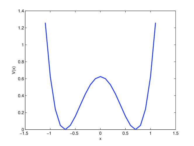
Figure 1: The potential in the first example.

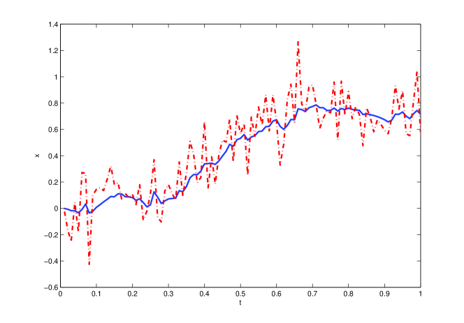
Figure 2: A random path (broken line) and its reconstruction by our filter (solid line).

For the $i$-the particle located at time $n\delta$ at $X^{n}_{i}$ the function $F(X)$ is

$$F(X)=(X-X^{n}_{i})^{2}/(2\sigma\delta)+(X-b^{n+1})^{2})^{2}/(2s),$$

which is always convex. A completion of a square yields $\min F=\phi=(1/2)(X^{n}_{i}-b^{n+1})^{2}/(\sigma\delta+s)$; the Jacobian $J$ is independent of the particle and need not be evaluated. In Figure 2 we display a particle run used to generate data and its reconstruction by our filter with $50$ particles. This figure is included for completeness but both of these paths are random, their difference varies from realization to realization, and may be large or small by accident. To get a quantitative estimate of the performance of the filter, we repeated this calculation $10^{4}$ times and computed the mean and the variance of the difference $\Delta$ between the run that generated the data and its reconstruction at time $t=1$, see Table I. This Table shows that the filter is unbiased and that the variance of $\Delta$ is comparable to the variance of the error in the observations $s=0.025$. Note that even with one single particle (and therefore no resampling) the results are still acceptable.

Table I

Mean and variance of the discrepancy between the observed path and the reconstructed path in example 1 as a function of the number of particles M, with $s=0.025$.

M	mean	variance
100	-.0001	.021
50	-.0001	.022
20	-.0001	.023
10	.0001	.024
5	-.0001	.027
1	-.0001	.038

We now discuss the relation between the posterior we wish to sample and the prior in several special cases, including non-convex situations. We want to produce samples of the pdf $P(x)=\exp(-F(x))/Z$, where $Z$ is a normalization constant and

$$F(x)=x^{2}/(2\sigma)+(h(x)-b)^{2}/(2s)$$ (10)

and $h(x)$ is a given function of $x$ (as in equation (2)) and $\sigma,s,b$ are given parameters. This can be viewed as a the first time step in time for a filtering problem where all the particles start from the same point so that $\exp(-F(x))/Z=P_{1}$, or as an analysis of the sampling for one particular particle in a general filtering problem, or as an instance of the more general problem of sampling a given pdf when the important events may be rare. In standard Bayesian sampling one samples the variable with pdf $\exp(-x^{2})/(2\sigma))/\sqrt{2\pi\sigma}$ and then one attaches to the sample at $x$ the weight $\exp(-(h(x)-b)^{2}/(2s))$; in an implicit sampler one finds a sample $x$ by solving $F(x)-\phi=\xi^{2}/2$ for a suitable $\phi$ and $\xi$ and attaching to the sample the weight $\exp(-\phi)J$. For given $\sigma,s$, the problem becomes more challenging as $|b|$ increases.

In both the standard and the implicit filters one can view the empirical pdf generated by the unweighted samples as a “prior” and the one generated by the weighted samples as the “posterior”. The difficulty with standard filters is that the prior and posterior densities may approach being mutually singular, so it is of interest to estimate the Radon-Nikodym derivative of one of these with respect to the other. If that derivative is a constant, we have achieved perfect importance sampling, as every neighborhood in the sample space is visited with a frequency proportional to its density. We estimate the Radon-Nikodym derivative of the prior with respect to the posterior as follows. In this simple problem one can evaluate the probability of any interval with respect to the posterior we wish to sample by quadratures. We divide the interval $[0,1]$ into $K$ pieces of equal lengths $1/K$, then find numerically points $Y_{1},Y_{2},\dots,Y_{K-1},$ with $Y_{K}=+\infty$, such that the posterior probability of the interval $[-\infty,Y_{k}]$ is $k/K$ for $k=1,2,\dots,K$. We then find $L=10^{5}$ samples of the prior and plot of a histogram of the frequencies with which these samples fall into the posterior equal probability intervals $(Y_{k-1},Y_{k})$. The more this histogram departs from being a constant independent of $k$, the more samples are needed to calculate the statistics of the posterior.

If $h(x)$ is linear, the weights in the implicit filter are all equal and the histogram is constant for all values of $b$. This remains true for all values of $b$, i.e., however far the observation $b$ is from what one may expect from the SDE alone. This is not the case with a standard Bayesian filter, where some parts of the sample space that have non-zero probability are visited very rarely. In Table II we list the histogram of frequencies for a linear observation function $h(x)=x$ and $b=2$ in a standard Bayesian filter, with K=10. We used $10^{4}$ samples; the fluctuations in the implicit case measure only the accuracy with which the histogram is computed with this number of samples.

Table II

Histogram of the Radon-Nikodym derivative of the prior with respect to the posterior, standard Bayesian filter vs. the implicit filter, 10000 particles, $b=2$, $\sigma=s=0.1$, $h(x)=x$.

k	standard	implicit
1	.987	.099
2	.006	.108
3	.002	.097
4	.001	.099
5	.004	.101
6	.003	.099
7	.001	.101
8	.001	.101
9	.000	.102
10	.000	.093

As a consequence, estimates obtained with the implicit filter are much more reliable than the ones obtained with the standard Bayesian filter. In Table III we list the estimates of the mean position of the linear problem as a function of b, with 30 particles, $\sigma=s=0.1$, for the standard Bayesian and the implicit filters, compared with the exact result. The standard deviations are not displayed, they are all near 0.01.

Table III

Comparison of the the estimates of the means, implicit vs. standard filter, $30$ particles, together with the exact results, linear case, as explained in the text.

b	exact	standard	implicit
0	0	-.05	.02
0.5	.25	.10	.27
1.	.5	.18	.51
1.5	.75	.23	.76
2.	1.	.26	1.01

The results in this one-dimensional problem mirror the situation with the example of Bickel et al. [2, 14], designed to display the breakdown of the standard Bayesian filter when the number of dimension is large; what happens there is that one particle hogs almost the whole weight, so that the number of particles needed grows catastrophically; in contrast, the implicit filter assigns equal weights to all the particles in any number of dimensions, so that the number of particles needed is independent of dimension, see also [6].

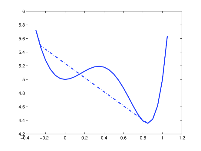
Figure 3: A non-convex function $F$ (solid line) and a $U$-shaped substitute (broken line).

We now turn to nonlinear and nonconvex examples. Let the observation function $h$ be strongly nonlinear: $h(x)=x^{3}$. With $\sigma=s=0.1$; the pdf (10) becomes non-$U$-shaped for $|b|\geq.77$. In Figure 3 we display the function $F$ for $b=1$ (the solid curve). To use the algorithms above we need a substitute function $F_{0}$ that is $U$-shaped; we also display in Figure 3 (the broken line) the function $F_{0}$ we used; the recipe here is to link a point above the local minimum on the left to the absolute minimum on the right by a straight line. There are many other possible constructions; the only general rule is to make the minimum of $F_{0}$ equal the absolute minimum of $F$, for obvious reasons. As described above, we solve $F_{0}(x)-\phi=\xi^{T}\xi/2$ and set $\phi=\min F_{0}+F_{0}(x)-F(x)$. It is important to note that this construction does not introduce any bias. The function $F_{0}$ constructed in this way is $U$-shaped but need not be convex, so that one needs algorithm (B) described above. In Table IV we compare the Radon-Nikodym derivatives of the prior with respect to the posterior for the resulting implicit sampling and for standard Bayesian sampling with $\sigma=s=0.1,b=1.5$.

Table IV

Radon-Nikodym derivatives of the prior with respect to the posterior, $h(x)=x^{3},\sigma=s=0.1,b=1.5,$ $10000$ samples, $F_{0}$ as in the text.

k	standard	explicit
1	.9948	.0899
2	.0028	.0537
3	.0011	.0502
4	.0004	.0563
5	.0003	.0696
6	.0002	.1860
7	.0001	.1107
8	.0001	.1194
9	.0001	.1196
10	0.	.1446

The histogram for the implicit filter is no longer perfectly balanced. The asymmetry in the histogram reflects the asymmetry of $F_{0}$ and can be eliminated by biasing $\xi$, but there is no reason to do so; there is enough importance sampling without this extra step.

In Table V we display the estimates of the means of the density for the two filters with 1000 particles for various values of $b$, compared with the exact results (the number of particles is relatively large because with $h(x)=x^{3}$ and our parameter choices the variance of the conditional density is significant, and this number of particles is needed for meaningful comparisons of either algorithm with the exact result).

Table V

Comparison of the the estimates of the means, implicit vs. standard filter, $1000$ particles, together with the exact result, when $h(x)=x^{3}$, as explained in the text.

b	exact	standard	implicit
0.	0.	-0.00 $\pm$.01	-.00 $\pm$.01
.5	.109	.109 $\pm$.01	.109$\pm$.01
1.0	.442	.394 $\pm$ .04	.451$\pm$.02
1.5	.995	.775$\pm$.09	.995$\pm$.01
2.0	1.18	.875$\pm$.05	1.18$\pm$.01
2.5	1.30	.895 $\pm$.02	1.29$\pm$.02

As mentioned in the previous section, there are alternatives to the replacement of $F$ by $F_{0}$; the point is that for each particle the function $F$ is an explicitly known non-random function, and this fact can be used in multiple ways.

6 Parameter identification

One important application of particle filters is to parameter identification, where the SDE contains an unknown parameter and the data are used to find this parameter’s value. One of the standard ways of doing this (see e.g [7]) is system augmentation: one adds to the SDE the equation $d\sigma=0$ for the unknown parameter $\sigma$, one offers $\sigma$ a gamut of possible values, and one relies on the resampling process that eliminate the values that do not fit the data. With the implicit filter this procedure fails, because the particles are not eliminated fast enough. The alternative we are proposing is finding the unknown parameter $\sigma$ by stochastic approximation. Specifically, Find a statistic $T$ of the output of the filter which is a function of $\sigma$, such that the expected value $E[T]$ vanishes when $\sigma$ has the right value $\sigma^{*}$, and then solve the equation $E[T]=E[T(\sigma)]=0$ by the Robbins-Monro algorithm [13], in which the equation $E[T]=0$ is solved by the iteration:

$$\sigma_{n+1}=\sigma_{n}-\alpha_{n}T(\sigma_{n}),$$ (11)

where which converges when the coefficients $\alpha_{n}$ are such that $\sum\alpha_{n}\rightarrow\infty$ while $\sum\alpha_{n}^{2}$ remains bounded.

As a concrete example, consider the SDE $dx=dW$, where $W$ is Brownian motion with variance $\sigma$, discretized with time steps $\delta$, with observations $b^{n}=x^{n}+\eta$, where $\eta$ is a Gaussian with mean zero and variance $s$. Data are generated by running the SDE once with the true value $\sigma^{*}$ of $\sigma$, adding the appropriate noise, and registering the result at time $n\delta$ as $b^{n}$ for $n=1,2,\dots,N$. For the functional $T$ we choose

$$T(\sigma)=C\sum(\Delta_{i}\Delta_{i-1})/\left((\sum\Delta_{i}^{2})(\sum\Delta^{2}_{i-1})\right)^{1/2},$$ (12)

where the summations are over $i$ between $2$ and $N$, $\Delta_{i}$ is the estimate of the increment of $x$ in the $i$-the step and $C$ is a scaling constant. Clearly if the $\sigma$ used in the filtering equals $\sigma^{*}$ then by construction the successive values of $\Delta_{i}$ are independent and $E[T]=0.$. We picked the parameters $N=100,\sigma=10^{-2},s=10^{-4},\delta=0.01$ (so that that the increment of $W$ in one step has variance $10^{-4}$).

Our algorithm is as follows: We make a guess $\sigma_{1}$, run the filter for $N$ steps, evaluate $T$, and make a new guess for $\sigma$ using equation (11) and $a_{1}=1$, rerun the filter, etc., with the $a_{n}$, the coefficient in equation (11) at the $n$-th step, equal to $1/n$. The scaling factor in (11) was found by trial and error: if it is too large the iteration becomes unstable, if it is too small the convergence is slow; we settled on $C=4$.

This algorithm requires that the filter be run without either resampling or backward sampling, because resampling and backward sampling introduce correlations between successive values of the $\Delta_{i}$ and bias the values of $T$. In a long run, in particular in a strongly nonlinear setting, one may need resampling for the filter to stay on track, and this can be done by segmentation: divide the run of the filter into segments of some moderate length $L$, perform the summations in the definition of $T$ over that segment, then go back and run that segment with resampling, then proceed to the next segment, etc.

The first question is, how well is it possible in principle to reconstruct an unknown value of $\sigma$ from $N$ observations; this issue was already discussed in [5]. Given $100$ samples of a Gaussian variable of mean $0$ and variance $\sigma$, the variance reconstructed from the observations is a random variable of mean $\sigma$ and variance $.16\cdot\sigma$; $100$ observations do not contain enough information to reconstruct $\sigma$ perfectly. A good way to estimate the best result that can be achieved is to run the algorithm with the guess $\sigma_{1}$ equal to the exact value $\sigma^{*}$ with which the data were generated. When this was done, the estimate of $\sigma$ was $1.27\sigma^{*}$. This result indicates the achievable accuracy.

In Table VI we display the result of our algorithm when we start with the starting value $\sigma_{1}=10\sigma^{*}$ and with $50$ particles. Each iteration requires that one run the filter once.

Table VI

Convergence of the parameter identification algorithm.

Iteration	new estimate $\sigma/\sigma^{*}$
0	10.
1	.819
2	.943
3	1.02
4	1.05
5	1.08
6	1.10
7	1.13
8	1.15
9	1.16
10	1.17
11	1.18
12	1.18
13	1.18

7 Conclusions

We have presented the implicit filter for data assimilation, together with several algorithms for the solution of the algebraic equations, including cases with non-convex functions $F$, as well as an algorithm for parameter identification. The key idea in implicit sampling is to solve an algebraic equation of the form $F(X)-\phi=\xi^{T}\xi/2$ for every particle, where the function $F$ is explicitly known, $X$ is the new position of the particle, $\phi$ is an additive factor, and $\xi$ is a sample of a fixed reference pdf; $F$ varies from particle to particle and step to step. This construction makes it possible to guide the particles to the high-probability area one by one under a wide variety of circumstances. It is important to note that the equation that links $\xi$ to $X$ is underdetermined and its solution can be adapted for each particular problem.

Implicit sampling is of interest in particular because of its potential uses in high dimensional problems, which are only briefly alluded to in the present paper. The effectiveness of implicit sampling in high-dimensional settings depends on one’s ability to design maps $\xi\rightarrow x$ that satisfy the criteria above and are computationally efficient. The design of such maps is problem dependent and we will present examples in the context of specific applications.

Acknowledgements We would like to thank Prof. Jonathan Weare for asking penetrating questions and for making very useful suggestions, Prof. Robert Miller for good advice and encouragement, and Mr. G. Zehavi for performing some of the preliminary computations. This work was supported in part by the Director, Office of Science, Computational and Technology Research, U.S. Department of Energy under Contract No. DE-AC02-05CH11231, and by the National Science Foundation under grants DMS-0705910 and OCE-0934298.

References

- [1] M. Arulampalam, S. Maskell, N. Gordon, and T. Clapp, A tutorial on particle filters for online nonlinear/nongaussian Bayesian tracking, IEEE Trans. Sig. Proc. 50 (2002), pp 174–188.
- [2] P. Bickel, B. Li, and T. Bengtsson, Sharp failure rates for the bootstrap particle filter in high dimensions, IMS Collections: Pushing the Limits of Contemporary Statistics: Contributions in Honor of Jayanta K. Ghosh (2008), pp. 318-329.
- [3] A.J. Chorin, Monte Carlo without chains, Comm. Appl. Math. Comp. Sc. 3 (2008), pp. 77-93.
- [4] A.J. Chorin and J. Kominiarczuk , Markov field Monte Carlo with statistical projections on random graphs, and applications to spin systems, in preparation.
- [5] A.J. Chorin and X. Tu, Implicit sampling for particle filters, Prod. Nat. Acad. Sc. USA 106 (2009), pp. 17249-17254.
- [6] A.J. Chorin and X. Tu, Interpolation and iteration for nonlinear filters, in press, Math. Mod. Num. Anal. (2010).
- [7] A. Doucet, N. de Freitas and N. Gordon (eds), Sequential Monte Carlo Methods in Practice, Springer, NY, 2001.
- [8] A. Doucet, S. Godsill and C. Andrieu, On sequential Monte Carlo sampling methods for Bayesian filtering, Stat. Comp. 10 (2000), pp. 197-208.
- [9] G. Evensen, Data Assimilation: the Ensemble Kalman Filter, Springer, NY, 2009.
- [10] E. Isaacson and H. Keller, Analysis of Numerical Methods, Wiley, New York, 1966.
- [11] P. Kloeden and E. Platen, Numerical Solution of Stochastic Differential Equations, Springer, Berlin, 1992.
- [12] R. Miller, E. Carter, and S. Blue, Data assimilation into nonlinear stochastic systems, Tellus 51A (1999), pp. 167-194.
- [13] H. Robbins and S. Monro, A stochastic approximation method, Ann. Math. Stat.22 (1951), pp. 400-407.
- [14] C. Snyder, T. Bengtsson, P. Bickel, and J. Anderson, Obstacles to high-dimensional particle filtering, Mon. Wea. Rev. 136 (2008), pp. 4629–4640.
- [15] A.M. Stuart. Inverse problems: a Bayesian perspective, Acta Numerica (19), 2010. pp 451-559
- [16] J. Weare, Efficient Monte Carlo sampling by parallel marginalization, Proc. Nat. Acad. Sc. USA 104 (2007), pp. 12657–12662.
- [17] J. Weare, Particle filtering with path sampling and an application to a bimodal ocean current model, J. Comput. Phys. 228 (2009), pp. 4321-4331.
- [18] M. Zakai, On the optimal filtering of diffusion processes, Zeit. Wahrsch. 11 (1969), pp. 230-243.