Elements of mathematical foundations for a numerical approach for weakly random homogenization problems

Abstract

This work is a follow-up to our previous work [2]. It extends and complements, both theoretically and experimentally, the results presented there. Under consideration is the homogenization of a model of a weakly random heterogeneous material. The material consists of a reference periodic material randomly perturbed by another periodic material, so that its homogenized behavior is close to that of the reference material. We consider laws for the random perturbations more general than in [2]. We prove the validity of an asymptotic expansion in a certain class of settings. We also extend the formal approach introduced in [2]. Our perturbative approach shares common features with a defect-type theory of solid state physics. The computational efficiency of the approach is demonstrated.

Keywords: Homogenization; Random Media; Defects

AMS Subject Classification: 35B27; 35J15; 35R60; 82D30

1 Introduction

Our purpose is to follow up on our previous study [2]. Let us recall, for consistency, that we consider homogenization for the following elliptic problem

$$\left\{\begin{aligned} &-\mathrm{div}\left((A_{per}(\frac{x}{\epsilon})+b_{\eta}(\frac{x}{\epsilon},\omega)C_{per}(\frac{x}{\epsilon}))\nabla u_{\epsilon}\right)=f(x)\;\mathrm{in}\;\mathcal{D}\subset{\mathbb{R}^{d}},\\ &u_{\epsilon}=0\;\mathrm{on}\;\partial\mathcal{D},\end{aligned}\right.$$ (1.1)

where the tensor $A_{per}$ models a reference $\mathbb{Z}^{d}$-periodic material which is randomly perturbed by the $\mathbb{Z}^{d}$-periodic tensor $C_{per}$, the stochastic nature of the problem being encoded in the stationary ergodic scalar field $b_{\eta}$ (the latter getting small when $\eta$ vanishes). We have studied in [2] the case of a perturbation that has a Bernoulli law with parameter $\eta$, meaning that $b_{\eta}$ is equal to $1$ with probability $\eta$ and $0$ with probability $1-\eta$. In the present work, we address more general laws. The common setting is that all the perturbations we consider are, to some extent, rare events which, although rare, modify the homogenized properties of the material. Our approach is a perturbative approach, and consists in approximating the stochastic homogenization problem for

$$A_{\eta}(x,\omega)=A_{per}(x)+b_{\eta}\left(x,\omega\right)C_{per}$$

using the periodic homogenization problem for $A_{per}$. In short, let us say that our main contribution is to derive an expansion

$$A_{\eta}^{*}=A_{per}^{*}+\eta\bar{A_{1}^{*}}+\eta^{2}\bar{A_{2}^{*}}+o(\eta^{2}),$$ (1.2)

where $A_{\eta}^{*}$ and $A_{per}^{*}$ are the homogenized tensors associated with $A_{\eta}$ and $A_{per}$ respectively, and the first and second-order corrections $\bar{A_{1}^{*}}$ and $\bar{A_{2}^{*}}$ can be, loosely speaking, computed in terms of the microscopic properties of $A_{per}$ and $C_{per}$ and the statistics of second order of the random field $b_{\eta}$. The formulation is made precise in [2] and in Sections 2 and 3 below.

Motivations behind setting (1.1), as well as a review of the mathematical literature on similar issues and a comprehensive bibliography, can be found in [2]. We complement our study of the perturbative approach introduced with [2] in two different directions.

In Section 2, we rigorously establish an asymptotic expansion of the homogenized tensor in a mathematical setting where our input parameter (the field $b_{\eta}$ in (1.1)) enjoys appropriate weak convergence properties, as $\eta$ vanishes, in a reflexive Banach space, namely a Lebesgue space $L^{\infty}({\mathcal{D}},L^{p}(\Omega))$ (with $p>1$). In such a setting, we are in position to rigorously prove a first order asymptotic expansion (announced in [3] and precisely stated in [3, Théorème 2.1] and Theorem 2 below) for the homogenization of $A_{\eta}$, using simple functional analysis techniques very similar to those exposed in [4]. In our Corollaries 3 and 4, the expansion is pushed to second order under additional assumptions.

Our aim in Section 3 is to further extend our formal theory of [2]. Recall that this formal theory, rather than manipulating the random field $b_{\eta}$ itself, consists in focusing on its law. We indeed assume that the image measure (the law) corresponding to the perturbation admits an expansion (see (3.4) below) with respect to $\eta$ in the sense of distributions. While [2] has only addressed the specific case of a Bernoulli law, we consider here more general laws and proceed with the same formal derivations. These derivations lead to a first-order correction $\bar{A_{1}^{*}}$ in (1.2) obtained as the limit when $N\rightarrow\infty$ of a sequence of tensors $A_{1}^{*,N}$ computed on the supercell $[-\frac{N}{2},\frac{N}{2}]^{d}$. It is the purpose of Proposition 7 to prove the convergence of $A_{1}^{*,N}$. The second-order term $\bar{A_{2}^{*}}$ is likewise defined as a limit, up to extraction, of a sequence of tensors $A_{2}^{*,N}$ when $N\rightarrow\infty$. The proof of the boundedness of the sequence $A_{2}^{*,N}$ and thus of its convergence up to extraction is not given here for it involves long and technical computations. We refer to [1] for the details. As in [2], our approach in this Section exhibits close ties with classical defect-type theories used in solid state physics.

We emphasize that, in sharp contrast to the exact stochastic homogenization of $A_{\eta}$, the determination of the first and second-order terms in (1.2) relies on entirely deterministic computations, albeit of very different kind, for both approaches of Sections 2 and 3.

Finally, a comprehensive series of numerical tests in Section 4 show, beyond those contained in [2], that the two approaches exposed here are efficient and quite robust: the computational workload induced by the perturbative approach is light compared to the direct homogenization of [2], and expansion (1.2) proves to be accurate for not so small perturbations.

We complement the text by a long appendix. The reader less interested in theoretical issues can easily omit the reading of this appendix. Besides providing, in Sections 5.1 and 5.2 and for consistency, some theoretical results useful in the body of the text, the purpose of this appendix is two-fold. We examine in details in Section 5.3 the one-dimensional setting, and we show that, expectedly, all our formal expansions can be made rigorous through explicit computations. We next demonstrate, in Section 5.4, that our two modes of derivation coincide in a particular setting appropriate for both the theoretical results of Section 2 and the formal results of Section 3. This final section therefore provides a proof of our formal manipulations of Section 3, in a setting – we concede it – that is not the setting the approach was designed to specifically address. Definite conclusions on the theoretical validity of the approach developped in Section 3 are yet to be obtained, even though applicability and efficiency are beyond doubt.

Throughout this paper, and unless otherwise mentioned, $C$ denotes a constant that depends at most on the ambient dimension $d$, and on the tensors $A_{per}$ and $C_{per}$. We write $C(\gamma)$ when $C$ depends on $\gamma$ and possibly on $d$, $A_{per}$ and $C_{per}$. The indices $i$ and $j$ denote indices in $\llbracket 1,d\rrbracket$.

2 A model of a weakly randomly perturbed material

For consistency, we first recall the general setting of our related work [2].

Throughout this article $\left(\Omega,\mathcal{F},\mathbb{P}\right)$ denotes a probability space with $\mathbb{P}$ the probability measure and $\omega\in\Omega$ an event. We denote by $\mathbb{E}(X)$ the expectation of a random variable $X$ and $Var(X)$ its variance.

We assume that the group $(\mathbb{Z}^{d},+)$ acts on $\Omega$ and denote by $\tau_{k},k\in\mathbb{Z}^{d},$ the group action. We also assume that this action is measure-preserving, that is,

$$\forall\mathcal{A}\in\mathcal{F},\forall k\in\mathbb{Z}^{d},\;\mathbb{P}(\mathcal{A})=\mathbb{P}(\tau_{k}\mathcal{A}),$$

and ergodic:

$$\forall\mathcal{A}\in\mathcal{F},(\forall k\in\mathbb{Z}^{d},\mathcal{A}=\tau_{k}\mathcal{A})\implies(\mathbb{P}(\mathcal{A})=0\;\mathrm{or}\;\mathbb{P}(\mathcal{A})=1).$$

We call $F\in L^{1}_{loc}(\mathbb{R}^{d},L^{1}(\Omega))$ stationary if

$$\forall k\in\mathbb{Z}^{d},\;F(x+k,\omega)=F(x,\tau_{k}\omega)\;\;\mathrm{almost\;everywhere\;in\;}x\in\mathbb{R}^{d}\;\mathrm{and\;}\omega\in\Omega.$$ (2.1)

Notice that if $F$ is deterministic, the notion of stationarity used here reduces to
$\mathbb{Z}^{d}$-periodicity, that is,

$$\forall k\in\mathbb{Z}^{d},F(x+k)=F(x)\;\;\mathrm{almost\;everywhere\;in\;}x\in\mathbb{R}^{d}.$$ (2.2)

We then consider the tensor field from $\mathbb{R}^{d}\times\Omega$ to $\mathbb{R}^{d\times d}$:

$$A_{\eta}(x,\omega)=A_{per}(x)+b_{\eta}(x,\omega)C_{per}(x),$$ (2.3)

where $A_{per}$ and $C_{per}$ are two deterministic $\mathbb{Z}^{d}$-periodic tensor fields and $b_{\eta}$ a stationary ergodic scalar field. The matrix $A_{per}$ models the reference periodic material, perturbed by $C_{per}$. This perturbation is random, thus the presence of $b_{\eta}$. We refer the reader to [4] for a more detailed presentation of the stationary ergodic setting in a similar weakly random framework.

We make the following assumptions on the random field $b_{\eta}$:

$$\exists M>0,\forall\eta>0,\|b_{\eta}\|_{L^{\infty}(Q\times\Omega)}\leq M,$$ (2.4)

$$\|b_{\eta}\|_{L^{\infty}(Q;L^{2}(\Omega))}\underset{\eta\rightarrow 0^{+}}{\rightarrow 0},$$ (2.5)

where $Q$ is the unit cell $[-\frac{1}{2},\frac{1}{2}]^{d}$.

Assumption (2.5) encodes that the perturbation for small $\eta$ is a rare event. Still, it is able to significantly modify the local structure of the material when it happens, for we do not require it to be small in $L^{\infty}(Q\times\Omega)$ as $\eta\rightarrow 0$.

We additionally assume that there exist $0<\alpha\leq\beta$ such that for all $\xi\in\mathbb{R}^{d}$, for almost all $x\in\mathbb{R}^{d}$ and for all $s\in[-M,M]$,

$$\alpha|\xi|^{2}\leq A_{per}(x)\xi\cdot\xi,\qquad\alpha|\xi|^{2}\leq\left(A_{per}+sC_{per}\right)(x)\xi\cdot\xi,$$ (2.6)

$$A_{per}(x)\xi|\leq\beta|\xi|,\qquad|\left(A_{per}+sC_{per}\right)(x)\xi|\leq\beta|\xi|.$$ (2.7)

We can therefore use the classical stochastic homogenization results (see for instance [7] for a comprehensive review or [2] for a concise presentation). The cell problems associated with (2.3) read

$$\left\{\begin{aligned} &-\mathrm{div}\left(A_{\eta}(\nabla w_{i}^{\eta}+e_{i})\right)=0\quad\mathrm{in}\,\,\mathbb{R}^{d},\\ &\nabla w_{i}^{\eta}\;\;\mathrm{stationary},\;\;\mathbb{E}\left(\int_{Q}\nabla w_{i}^{\eta}\right)=0.\end{aligned}\right.$$ (2.8)

Problem (2.8) has a solution unique up to the addition of a random constant. The function $w_{i}^{\eta}$ is called the $i$-th corrector or cell solution.

The homogenized tensor $A_{\eta}^{*}$ is given by

$$\forall i\in\llbracket 1,d\rrbracket,\;\;A_{\eta}^{*}e_{i}=\mathbb{E}\left(\int_{Q}A_{\eta}(\nabla w_{i}^{\eta}+e_{i})\right).$$ (2.9)

Throughout the rest of this paper we will denote by $w_{i}^{0}$ the $i$-th cell solution associated with $A_{per}$, defined up to an additive constant by

$$\left\{\begin{aligned} &-\mathrm{div}\left(A_{per}(\nabla w_{i}^{0}+e_{i})\right)=0\quad\mathrm{in}\,\,Q,\\ &w_{i}^{0}\;\;\mathbb{Z}^{d}-\mathrm{periodic}.\end{aligned}\right.$$ (2.10)

The periodic homogenized tensor is then given by

$$\forall i\in\llbracket 1,d\rrbracket,\;\;A_{per}^{*}e_{i}=\int_{Q}A_{per}(\nabla w_{i}^{0}+e_{i}).$$ (2.11)

Due to the specific form of $A_{\eta}$, the following zero-order result can be easily proved. The proof is actually the same as that in Lemma 1 of [2], which relies on the fact that $\|b_{\eta}\|_{L^{\infty}(Q;L^{2}(\Omega))}$ converges to $0$ as $\eta$ tends to $0$.

Lemma 1.

When $\eta\rightarrow 0$, $A_{\eta}^{*}\rightarrow A_{per}^{*}$.

Our goal is to find an asymptotic expansion for $A_{\eta}$ with respect to $\eta$, and a first answer is given by the following theorem announced as Théorème 1 in [3] :

Theorem 2 (Théorème 1, [3]).

Assume that $b_{\eta}$ satisfies (2.4) and (2.5), and denote by $m_{\eta}=\|b_{\eta}\|_{L^{\infty}(Q;L^{2}(\Omega))}$. There exists a subsequence of $\eta$, still denoted $\eta$ for the sake of simplicity, such that $\frac{b_{\eta}}{m_{\eta}}$ converges weakly-* in ${L^{\infty}(Q;L^{2}(\Omega))}$ to a limit field denoted by $\bar{b}_{0}$ when $n\rightarrow 0$. Then

• for all $i\in\llbracket 1,d\rrbracket$, the following expansion

  $$\nabla w_{i}^{\eta}=\nabla w_{i}^{0}+m_{\eta}\nabla v_{i}^{0}+o(m_{\eta})$$ (2.12)

  holds weakly in $L^{2}(Q;L^{2}(\Omega))$, where $w_{i}^{0}$ is the solution to the $i$-th periodic cell problem and $v_{i}^{0}$ is solution to

  $$\left\{\begin{aligned} &-\mathrm{div}(A_{per}\nabla v_{i}^{0})=\mathrm{div}\left(\bar{b}_{0}C_{per}(\nabla w^{0}+e_{i})\right)\quad\mathrm{in}\,\,\mathbb{R}^{d},\\ &\nabla v_{i}^{0}\;\;\mathrm{stationary},\;\mathbb{E}\left(\int_{Q}\nabla v_{i}^{0}\right)=0.\end{aligned}\right.$$ (2.13)

• $A_{\eta}^{*}$ can be expanded up to first order as

  $$A_{\eta}^{*}=A_{per}^{*}+m_{\eta}\tilde{A_{1}^{*}}+o(m_{\eta}),$$ (2.14)

  where

  $$\forall i\in\llbracket 1,d\rrbracket,\;\tilde{A_{1}^{*}}e_{i}=\int_{Q}\mathbb{E}(\bar{b}_{0})C_{per}(\nabla w_{i}^{0}+e_{i})+\int_{Q}A_{per}\nabla\mathbb{E}(v_{i}^{0}).$$ (2.15)

Proof.

We fix $i\in\llbracket 1,d\rrbracket$ and define $v_{i}^{\eta}=\frac{w_{i}^{\eta}-w_{i}^{0}}{m_{\eta}}$. $v_{i}^{\eta}$ is solution to

$$\left\{\begin{aligned} &-\mathrm{div}\left(A_{\eta}\nabla v_{i}^{\eta}\right)=\mathrm{div}\left(\frac{b_{\eta}}{m_{\eta}}C_{per}\left(\nabla w_{i}^{0}+e_{i}\right)\right)\quad\mathrm{in}\,\,\mathbb{R}^{d},\\ &\nabla v_{i}^{\eta}\;\;\mathrm{stationary},\;\mathbb{E}\left(\int_{Q}\nabla v_{i}^{\eta}\right)=0.\end{aligned}\right.$$ (2.16)

Using an argument similar to that used in the proof of Lemma 1 in [2], we have

$$\forall\eta>0,\,\,\|\nabla v_{i}^{\eta}\|_{L^{2}(Q\times\Omega)}\leq\frac{1}{\alpha}\|C_{per}\left(\nabla w_{i}^{0}+e_{i}\right)\|_{L^{2}(Q)}.$$

where $\alpha$ is defined in (2.6).

The sequence $\nabla v_{i}^{\eta}$ is bounded in $L^{2}(Q\times\Omega)$ and therefore, up to extraction, weakly converges in $L^{2}(Q\times\Omega)$ to some limit which is necessarily a gradient and which we denote $\nabla v_{i}^{0}$. Since $b_{\eta}$ converges strongly to $0$ in $L^{2}(Q\times\Omega)$, $b_{\eta}\nabla v_{i}^{\eta}$ converges to $0$ in $\mathcal{D}^{\prime}(Q\times\Omega)$. It is then easy to pass to the limit $\eta\rightarrow 0$ in (2.16) and to deduce that $v_{i}^{0}$ is solution to

$$\left\{\begin{aligned} &-\mathrm{div}\left(A_{per}\nabla v_{i}^{0}\right)=\mathrm{div}\left(\bar{b}_{0}C_{per}\left(\nabla w_{i}^{0}+e_{i}\right)\right)\quad\mathrm{in}\,\,\mathbb{R}^{d},\\ &\nabla v_{i}^{0}\;\;\mathrm{stationary},\;\mathbb{E}\left(\int_{Q}\nabla v_{i}^{0}\right)=0.\end{aligned}\right.$$

Thus $\frac{\nabla w_{i}^{\eta}-\nabla w_{i}^{0}}{m_{\eta}}$ converges, up to extraction, weakly to $\nabla v_{i}^{0}$ in $L^{2}(Q\times\Omega)$. This amounts to say that we have the following first-order expansion:

$$\nabla w_{i}^{\eta}=\nabla w_{i}^{0}+m_{\eta}\nabla v_{i}^{0}+o(m_{\eta})\quad\mathrm{in}\;L^{2}(Q\times\Omega)\;\mathrm{weak}.$$

Inserting this expansion in (2.9), we obtain

$$A_{\eta}^{*}e_{i} = A_{per}^{*}e_{i}+m_{\eta}\int_{Q}\mathbb{E}(\bar{b}_{0})C_{per}(\nabla w_{i}^{0}+e_{i})+m_{\eta}\int_{Q}A_{per}\nabla\mathbb{E}(v_{i}^{0})+o(m_{\eta}),$$

which concludes the proof.

∎

Remark 1.

Notice that taking the expectation of both sides of (2.13), $\mathbb{E}(v_{i}^{0})$ is actually the $\mathbb{Z}^{d}$-periodic function that is the unique solution (up to an additive constant) to

$$\left\{\begin{aligned} &-\mathrm{div}\left(A_{per}\nabla\mathbb{E}(v_{i}^{0})\right)=\mathrm{div}\left(\mathbb{E}(\bar{b}_{0})C_{per}\left(\nabla w_{i}^{0}+e_{i}\right)\right)\quad\mathrm{in}\,\,Q,\\ &\mathbb{E}(v_{i}^{0})\;\;\mathbb{Z}^{d}-\mathrm{periodic}.\\ \end{aligned}\right.$$ (2.17)

The computation of $A_{\eta}^{*}$ up to the first order in $m_{\eta}$ only requires solving $2d$ deterministic problems, namely (2.10) and (2.17), in the unit cell $Q$.

In fact, the situation is even more advantageous when $A_{per}$ is a symmetric matrix, as shown by our next remark.

Remark 2.

Defining the adjoint problems to the cell problems (2.10),

$$\left\{\begin{aligned} &-\mathrm{div}\left(A_{per}^{T}(\nabla\tilde{w}_{i}^{0}+e_{i})\right)=0\quad\mathrm{in}\,\,Q,\\ &\tilde{w}_{i}^{0}\;\;\mathbb{Z}^{d}-\mathrm{periodic},\end{aligned}\right.$$ (2.18)

where we have denoted by $A_{per}^{T}$ the transposed matrix of $A_{per}$, allows to write the first-order correction (2.15) in a slightly different form. Indeed, multiplying (2.17) by $\tilde{w}_{j}^{0}$ and integrating by parts, we obtain

$$\int_{Q}A_{per}\nabla\mathbb{E}(v_{i}^{0})\cdot\nabla\tilde{w}_{j}^{0}=-\int_{Q}\mathbb{E}(\bar{b}_{0})C_{per}\left(\nabla w_{i}^{0}+e_{i}\right)\cdot\nabla\tilde{w}_{j}^{0}.$$

Likewise, multiplying (2.18) by $\nabla\mathbb{E}(v_{i}^{0})$ and integrating by parts yields

$$\int_{Q}A_{per}\nabla\mathbb{E}(v_{i}^{0})\cdot\left(\nabla\tilde{w}_{j}^{0}+e_{j}\right)=0.$$

Combining these equalities gives

$$\int_{Q}A_{per}\nabla\mathbb{E}(v_{i}^{0})\cdot e_{j}=\int_{Q}\mathbb{E}(\bar{b}_{0})C_{per}\left(\nabla w_{i}^{0}+e_{i}\right)\cdot\nabla\tilde{w}_{j}^{0},$$

and thus (2.15) may be equivalently phrased as

$$\forall(i,j)\in\llbracket 1,d\rrbracket^{2},\;\tilde{A_{1}^{*}}e_{i}\cdot e_{j} = \int_{Q}\mathbb{E}(\bar{b}_{0})C_{per}(\nabla w_{i}^{0}+e_{i})\cdot(\nabla\tilde{w}_{j}^{0}+e_{j}).$$ (2.19)

When $A_{per}$ is symmetric, $\tilde{w}_{j}^{0}=w_{j}^{0}$, and solving the periodic cell problems (2.10) suffices to determine $A_{\eta}^{*}$ up to the first order in $m_{\eta}$.

Pushing expansion (2.14) to second order requires more information on $b_{\eta}$:

Corollary 3.

Assume in addition to (2.4) and (2.5) that

$$b_{\eta}=\eta\bar{b}_{0}+\eta^{2}\bar{r}_{0}+o(\eta^{2})\quad\mathrm{weakly}-^{*}\;\mathrm{in\;}L^{\infty}(Q;L^{2}(\Omega)).$$ (2.20)

Then

• for all $i\in\llbracket 1,d\rrbracket$, the following expansion

  $$\nabla w_{i}^{\eta}=\nabla w_{i}^{0}+\eta\nabla v_{i}^{0}+\eta^{2}\nabla z_{i}^{0}+o(\eta^{2})$$ (2.21)

  holds weakly in $L^{2}(Q;L^{2}(\Omega))$, where $z_{i}^{0}$ is solution to

  $$\left\{\begin{aligned} &-\mathrm{div}(A_{per}\nabla z_{i}^{0})=\mathrm{div}\left(\bar{r}_{0}C_{per}(\nabla w_{i}^{0}+e_{i})\right)+\mathrm{div}\left(\bar{b}_{0}C_{per}\nabla v_{i}^{0}\right)\quad\mathrm{in}\,\,\mathbb{R}^{d},\\ &\nabla z_{i}^{0}\;\;\mathrm{stationary},\;\mathbb{E}\left(\int_{Q}\nabla z_{i}^{0}\right)=0.\end{aligned}\right.$$ (2.22)

• $A_{\eta}^{*}$ can be expanded up to second order as

  $$A_{\eta}^{*}=A_{per}^{*}+\eta\tilde{A_{1}^{*}}+\eta^{2}\tilde{A_{2}^{*}}+o(\eta^{2}),$$ (2.23)

  where $\tilde{A_{1}^{*}}$ is defined by (2.15) and for all $i\in\llbracket 1,d\rrbracket$,

  $$\tilde{A_{2}^{*}}e_{i}=\int_{Q}\mathbb{E}(\bar{r}_{0})C_{per}(\nabla w_{i}^{0}+e_{i})+\eta^{2}\int_{Q}C_{per}\mathbb{E}(\bar{b}_{0}\nabla v_{i}^{0})+\int_{Q}A_{per}\nabla\mathbb{E}(z_{i}^{0}),$$ (2.24)

or equivalently, for all $(i,j)\in\llbracket 1,d\rrbracket^{2}$,

$$\tilde{A_{2}^{*}}e_{i}\cdot e_{j}=\int_{Q}\mathbb{E}(\bar{r}_{0})C_{per}(\nabla w_{i}^{0}+e_{i})\cdot(\nabla\tilde{w_{j}}^{0}+e_{j})+\int_{Q}C_{per}\mathbb{E}(\bar{b}_{0}\nabla v_{i}^{0})\cdot(\nabla\tilde{w_{j}}^{0}+e_{j}).$$ (2.25)

Proof.

The proof follows the same pattern as that of Theorem 2. The computation of the second order relies on the fact that (2.20) implies that $\frac{b_{\eta}}{\eta}$ converges strongly to $\bar{b}_{0}$ in $L^{\infty}(Q;L^{2}(\Omega))$, whereas the convergence was weak in Theorem 2. Likewise, the expansion of the cell solution, namely (2.21), implies that $\frac{\nabla w_{i}^{\eta}-\nabla w_{i}^{0}}{\eta}$ converges strongly to $\nabla v_{i}^{0}$ in $L^{2}(Q;L^{2}(\Omega))$. We then obtain (2.23) and (2.24) by inserting (2.21) in (2.9), and deduce (2.25) from (2.24) as in Remark 2. ∎

The computation of $A_{\eta}^{*}$ up to the order $\eta^{2}$ is much more intricate than that up to the order $\eta$, for it requires determining $\mathbb{E}(\bar{b}_{0}\nabla v_{i}^{0})$. Computing the periodic deterministic function $\mathbb{E}(v_{i}^{0})$ solution to the simpler problem (2.17) is not sufficient in general. We have to determine the stationary random field $v_{i}^{0}$ solution to (2.13) in $\mathbb{R}^{d}$.

It turns out that in a particular, practically relevant setting, we may still avoid solving the random problem (2.13). This setting presents the additional advantage to provide insight on the influence of spatial correlation.

Corollary 4.

Assume that $b_{\eta}$ is uniform in each cell of $\mathbb{Z}^{d}$, and writes

$$b_{\eta}(x,\omega)=\sum_{k\in\mathbb{Z}^{d}}\mathds{1}_{Q+k}(x)B_{\eta}(\tau_{k}\omega),$$ (2.26)

where $B_{\eta}$ satisfies

$$\forall\eta>0,\|B_{\eta}\|_{L^{\infty}(\Omega)}\leq M,$$ (2.27)

$$B_{\eta}=\eta\bar{B}_{0}+\eta^{2}\bar{R}_{0}+o(\eta^{2})\quad\mathrm{weakly\;in\;}L^{2}(\Omega).$$ (2.28)

Assume also that

$$\sum_{k\in\mathbb{Z}^{d}}|cov(\bar{B}_{0},\bar{B}_{0}(\tau_{k}\cdot))|<\infty.$$ (2.29)

Then the second-order term (2.25) can be rewritten

$$\begin{aligned} \tilde{A_{2}^{*}}e_{i}\cdot e_{j}=&\mathbb{E}(\bar{R}_{0})\int_{Q}C_{per}(\nabla w_{i}^{0}+e_{i})\cdot(\nabla\tilde{w_{j}}^{0}+e_{j})+Var(\bar{B}_{0})\int_{Q}C_{per}\nabla t_{i}\cdot(\nabla\tilde{w}_{j}^{0}+e_{j})\\ &+(\mathbb{E}(\bar{B}_{0}))^{2}\int_{Q}C_{per}\nabla s_{i}\cdot(\nabla\tilde{w}_{j}^{0}+e_{j})\\ &+\sum_{k\in\mathbb{Z}^{d},k\neq 0}cov(\bar{B}_{0},\bar{B}_{0}(\tau_{k}\cdot))\int_{Q}C_{per}\nabla t_{i}(\cdot-k)\cdot(\nabla\tilde{w}_{j}^{0}+e_{j}),\end{aligned}$$ (2.30)

where $t_{i}$ is a $L^{2}_{loc}(\mathbb{R}^{d})$ function solving

$$\left\{\begin{aligned} &-\mathrm{div}\left(A_{per}\nabla t_{i}\right)=\mathrm{div}\left(C_{per}\mathds{1}_{Q}\left(\nabla w_{i}^{0}+e_{i}\right)\right)\quad\mathrm{in}\,\,\mathbb{R}^{d},\\ &\nabla t_{i}\in L^{2}(\mathbb{R}^{d}),\end{aligned}\right.$$ (2.31)

and $s_{i}$ solves

$$\left\{\begin{aligned} &-\mathrm{div}\left(A_{per}\nabla s_{i}\right)=\mathrm{div}\left(C_{per}\left(\nabla w_{i}^{0}+e_{i}\right)\right)\quad\mathrm{in}\,\,Q,\\ &s_{i}\;\;\mathbb{Z}^{d}-\mathrm{periodic}.\end{aligned}\right.$$ (2.32)

Proof.

We notice first that the specific form (2.26) of $b_{\eta}$ considered implies that $\bar{b}_{0}$ and $\bar{r}_{0}$ defined in (2.20) here write

$$\bar{b}_{0}(x,\omega)=\sum_{k\in\mathbb{Z}^{d}}\mathds{1}_{Q+k}(x)\bar{B}_{0}(\tau_{k}\omega),$$ (2.33)

$$\bar{r}_{0}(x,\omega)=\sum_{k\in\mathbb{Z}^{d}}\mathds{1}_{Q+k}(x)\bar{R}_{0}(\tau_{k}\omega).$$ (2.34)

The rest of the proof mainly consists in showing that in this particular setting, $\nabla v_{i}^{0}$ and the product $\bar{b}_{0}\nabla v_{i}^{0}$ can be written using the deterministic functions $t_{i}$ and $s_{i}$. The existence of $t_{i}$ and its uniqueness up to an additive constant come from Lemmas 6 and 7 in [2].

We start by proving that the sum

$$\sum_{k\in\mathbb{Z}^{d}}\left(\bar{B}_{0}(\tau_{k}\omega)-\mathbb{E}(\bar{B}_{0})\right)\nabla t_{i}(x-k)$$ (2.35)

is a convergent series in $L^{2}(Q\times\Omega)$.

To this end, we compute the norm of the remainder of this series:

$$\begin{aligned} &\left\|\sum_{|k|\geq N}\left(\bar{B}_{0}(\tau_{k}\cdot)-\mathbb{E}(\bar{B}_{0})\right)\nabla t_{i}(\cdot-k)\right\|^{2}_{L^{2}(Q\times\Omega)}\\ &=\sum_{|k|\geq N}\sum_{|l|\geq N}cov(\bar{B}_{0}(\tau_{k}\cdot),\bar{B}_{0}(\tau_{l}\cdot))\int_{Q}\nabla t_{i}(\cdot-k)\nabla t_{i}(\cdot-l)\\ &\leq\frac{1}{2}\sum_{|k|\geq N}\sum_{|l|\geq N}|cov(\bar{B}_{0}(\tau_{k}\cdot),\bar{B}_{0}(\tau_{l}\cdot))|(\|\nabla t_{i}(\cdot-k)\|_{L^{2}(Q)}^{2}+\|\nabla t_{i}(\cdot-l)\|_{L^{2}(Q)}^{2})\\ &\leq\sum_{|k|\geq N}\sum_{|l|\geq N}|cov(\bar{B}_{0}(\tau_{k}\cdot),\bar{B}_{0}(\tau_{l}\cdot))|\,\|\nabla t_{i}(\cdot-k)\|_{L^{2}(Q)}^{2}\\ &\leq\sum_{|k|\geq N}\left(\|\nabla t_{i}(\cdot-k)\|_{L^{2}(Q)}^{2}\sum_{|l|\geq N}|cov(\bar{B}_{0}(\tau_{k}\cdot),\bar{B}_{0}(\tau_{l}\cdot))|\right)\\ &\leq\sum_{|k|\geq N}\left(\|\nabla t_{i}(\cdot-k)\|_{L^{2}(Q)}^{2}\sum_{|l|\geq N}|cov(\bar{B}_{0},\bar{B}_{0}(\tau_{l-k}\cdot))|\right)\\ &\leq\sum_{|k|\geq N}\|\nabla t_{i}(\cdot-k)\|_{L^{2}(Q)}^{2}\sum_{k\in\mathbb{Z}^{d}}|cov(\bar{B}_{0},\bar{B}_{0}(\tau_{k}\cdot))|.\end{aligned}$$

Using (2.29), we obtain

$$\left\|\sum_{|k|\geq N}\left(\bar{B}_{0}(\tau_{k}\cdot)-\mathbb{E}(\bar{B}_{0})\right)\nabla t_{i}(\cdot-k)\right\|^{2}_{L^{2}(Q\times\Omega)}\leq C\sum_{|k|\geq N}\|\nabla t_{i}(\cdot-k)\|_{L^{2}(Q)}^{2}.$$ (2.36)

Since $\nabla t_{i}\in L^{2}(\mathbb{R}^{d})$, the right-hand side of (2.36) converges to zero when $N$ goes to infinity.

Consequently, (2.35) defines a vector $T$ in $L^{2}(Q\times\Omega)$. It is clear from (2.35) that $\frac{\partial T_{p}}{\partial x_{n}}=\frac{\partial T_{n}}{\partial x_{p}}$ for all $(n,p)\in\llbracket 1,d\rrbracket^{2}$. Thus $T$ is a gradient, and there exists a function $\tilde{v}_{i}$ such that

$$\nabla\tilde{v}_{i}=T+\mathbb{E}(\bar{B}_{0})\nabla s_{i}=\sum_{k\in\mathbb{Z}^{d}}\left(\bar{B}_{0}(\tau_{k}\cdot)-\mathbb{E}(\bar{B}_{0})\right)\nabla t_{i}(x-k)+\mathbb{E}(\bar{B}_{0})\nabla s_{i}.$$ (2.37)

Since $s_{i}$ is $\mathbb{Z}^{d}$-periodic, we deduce from (2.37) that

$$\nabla\tilde{v}_{i}\;\mathrm{is\;stationary\;and\;}\mathbb{E}\left(\int_{Q}\nabla\tilde{v}_{i}\right)=0.$$ (2.38)

We then compute, using (2.31) and (2.32),

$$-\mathrm{div}(A_{per}\nabla\tilde{v}_{i}) = \sum_{k\in\mathbb{Z}^{d}}-\mathrm{div}(A_{per}\nabla t_{i}(\cdot-k))\left(\bar{B}_{0}(\tau_{k}\cdot)-\mathbb{E}(\bar{B}_{0})\right)$$ (2.39)

$$-\mathrm{div}(A_{per}\nabla s_{i})\mathbb{E}(\bar{B}_{0})$$

$$= \sum_{k\in\mathbb{Z}^{d}}\mathrm{div}\left(C_{per}\mathds{1}_{Q+k}\left(\nabla w_{i}^{0}+e_{i}\right)\right)\left(\bar{B}_{0}(\tau_{k}\cdot)-\mathbb{E}(\bar{B}_{0})\right)$$

$$+\mathrm{div}\left(C_{per}\left(\nabla w_{i}^{0}+e_{i}\right)\right)\mathbb{E}(\bar{B}_{0})$$

$$= \sum_{k\in\mathbb{Z}^{d}}\mathrm{div}\left(C_{per}\mathds{1}_{Q+k}\,\bar{B}_{0}(\tau_{k}\cdot)\left(\nabla w_{i}^{0}+e_{i}\right)\right).$$

Because of (2.33), (2.39) implies

$$-\mathrm{div}(A_{per}\nabla\tilde{v}_{i})=\mathrm{div}\left(\bar{b}_{0}C_{per}(\nabla w^{0}+e_{i})\right).$$ (2.40)

It follows from (2.38) and (2.40) that $\tilde{v}_{i}$ solves (2.13). As (2.13) has a solution unique up to the addition of a random constant, we obtain

$$\nabla v_{i}^{0}=\nabla\tilde{v}_{i}=\sum_{k\in\mathbb{Z}^{d}}\left(\bar{B}_{0}(\tau_{k}\cdot)-\mathbb{E}(\bar{B}_{0})\right)\nabla t_{i}(x-k)+\mathbb{E}(\bar{B}_{0})\nabla s_{i}.$$ (2.41)

We deduce from (2.33) and (2.41) that

$$\mathbb{E}(\bar{b}_{0}\nabla v_{i}^{0}) = \sum_{k\in\mathbb{Z}^{d}}\sum_{l\in\mathbb{Z}^{d}}\mathds{1}_{Q+l}\,\mathbb{E}(\bar{B}_{0}(\tau_{l}\cdot)(\bar{B}_{0}(\tau_{k}\cdot)-\mathbb{E}(\bar{B}_{0})))\nabla t_{i}(\cdot-k)$$

$$+(\mathbb{E}(\bar{B}_{0}))^{2}\sum_{l\in\mathbb{Z}^{d}}\mathds{1}_{Q+l}\nabla s_{i}$$

$$= \sum_{k\in\mathbb{Z}^{d}}\sum_{l\in\mathbb{Z}^{d}}\mathds{1}_{Q+l}\,cov(\bar{B}_{0}(\tau_{k}\cdot),\bar{B}_{0}(\tau_{l}\cdot))\nabla t_{i}(\cdot-k)+(\mathbb{E}(\bar{B}_{0}))^{2}\sum_{l\in\mathbb{Z}^{d}}\mathds{1}_{Q+l}\nabla s_{i},$$

and then that

$$\begin{aligned} \mathds{1}_{Q}\mathbb{E}(\bar{b}_{0}\nabla v_{i}^{0})=&Var(\bar{B}_{0})\nabla t_{i}+\sum_{k\in\mathbb{Z}^{d},k\neq 0}cov(\bar{B}_{0}(\cdot),\bar{B}_{0}(\tau_{k}\cdot))\nabla t_{i}(\cdot-k)\\ &+(\mathbb{E}(\bar{B}_{0}))^{2}\nabla s_{i}.\end{aligned}$$ (2.42)

We conclude by inserting (2.34) and (2.42) in (2.25).

∎

Theorem 2 (and its two corollaries) are only of interest if $\mathbb{E}(\bar{b}_{0})\neq 0$. Indeed, if $\mathbb{E}(\bar{b}_{0})=0$ it only states that $A_{\eta}^{*}=A_{per}^{*}+o(m_{\eta})$.

The prototypical case where Theorem 2 does not provide valuable information is the case studied in [2]: $b_{\eta}(x,\omega)=\sum_{k\in\mathbb{Z}^{d}}\mathds{1}_{Q+k}(x)B_{\eta}^{k}(\omega)$, where the $B_{\eta}^{k}$ are independent identically distributed variables that have Bernoulli law with parameter $\eta$, i.e are equal to 1 with probability $\eta$ and to 0 with probability $1-\eta$. Then, using the notation of Theorem 2, $b_{\eta}^{2}=b_{\eta}$, $m_{\eta}=\sqrt{\eta}$ and $\bar{b}_{0}=0$, and we only get $A_{\eta}^{*}=A_{per}^{*}+o(\sqrt{\eta})$ (while appendix 6.1 of [2] shows that there exists a tensor $\bar{A_{1}^{*}}$ such that $A_{\eta}^{*}=A_{per}^{*}+\eta\bar{A_{1}^{*}}+o(\eta)$ at least in dimension one). Omitting the dependence on the space variables since $b_{\eta}$ is uniform in each cell of $\mathbb{Z}^{d}$ in this particular setting, a suitable functional space $F$ on $\Omega$ to obtain a non trivial weak limit of $\frac{b_{\eta}}{\|b_{\eta}\|_{F}}$ would be $L^{1}(\Omega)$ for the norm of each $B_{\eta}^{k}$ in $L^{1}(\Omega)$ is equal to $\eta$. The Dunford-Petti weak compactness criterion in that space is however not satisfied by $\frac{b_{\eta}}{\|b_{\eta}\|_{L^{1}(\Omega)}}$. The reason is of course that $\frac{b_{\eta}}{\|b_{\eta}\|_{L^{1}(\Omega)}}$ converges in the set of bounded measures to a Dirac mass. The techniques used in the proof of Theorem 2 and its two corollaries thus do not work in this setting.

The above considerations somehow suggest that an alternative viewpoint might be useful. Because of (2.5), the image measure $dP_{\eta}^{x}$ of $b_{\eta}(x,\cdot)$ converges to a Dirac mass in the sense of distributions. Our alternate approach, related to our work [2], consists in working out an expansion of the image measure (or of the law), rather than an expansion of the random variable. Like in [2], our manipulations are mostly formal. Some rigorous foundations, in specific settings, are provided in the appendix.

3 A formal approach

3.1 A new assumption on the image measure

For simplicity, we assume as in Corollary 4 that $b_{\eta}$ is uniform in each cell of $\mathbb{Z}^{d}$, and is of the form

$$b_{\eta}(x,\omega)=\sum_{k\in\mathbb{Z}^{d}}\mathds{1}_{Q+k}(x)B_{\eta}^{k}(\omega),$$ (3.1)

where the $B_{\eta}^{k}$ are independent identically distributed random variables, the distribution of which is given by a "mother variable" $B_{\eta}$. For convenience we slightly modify (2.27) and require

$$\exists\epsilon>0,\forall\eta>0,\|B_{\eta}\|_{L^{\infty}(\Omega)}\leq M-\epsilon$$ (3.2)

$$\|B_{\eta}\|_{L^{2}(\Omega)}\underset{\eta\rightarrow 0}{\rightarrow 0}.$$ (3.3)

Assumption (3.2) is a technical assumption which implies in particular that for every $\eta>0$, the image measure $dP_{\eta}$ of $B_{\eta}$ is a distribution with compact support contained in the open set $]-M,M[$. Of course the specific values of $M$ and $\epsilon$ have no particular significance. Throughout the sequel we denote by $\mathcal{E}^{\prime}(]-M,M[)$ the space of distributions on $\mathbb{R}$ with compact support in $]-M,M[$, and by $\langle T,\varphi\rangle$ the action of a distribution $T\in\mathcal{E}^{\prime}(]-M,M[)$ on a test function $\varphi\in\mathcal{C}^{\infty}(]-M,M[)$. Basic elements of distribution theory are recalled in Section 5.1 of the appendix, for convenience of the reader not familiar with technical issues.

Because of assumption (3.3) and Lebesgue dominated convergence theorem, it is clear that for every $\varphi\in\mathcal{C}^{\infty}(]-M,M[)$,

$$\mathbb{E}(\varphi(B_{\eta}))\underset{\eta\rightarrow 0^{+}}{\rightarrow}\varphi(0).$$

Since $\mathbb{E}(\varphi(B_{\eta}))=\langle dP_{\eta},\varphi\rangle\;\mathrm{and}\;\varphi(0)=\langle\delta_{0},\varphi\rangle$ where $\delta_{0}$ is the Dirac mass at $0$, $dP_{\eta}$ converges to $\delta_{0}$ in $\mathcal{E}^{\prime}(]-M,M[)$.

This leads us to assume that $dP_{\eta}$ satisfies

$$dP_{\eta}=\delta_{0}+\eta d\bar{P}_{1}+\eta^{2}d\bar{P}_{2}+o(\eta^{2})\quad\mathrm{in}\;\mathcal{E}^{\prime}(]-M,M[),$$ (3.4)

which is equivalent to

$$\forall\varphi\in\mathcal{C}^{\infty}(]-M,M[),\;\mathbb{E}(\varphi(B_{\eta}))=\langle dP_{\eta},\varphi\rangle=\varphi(0)+\eta\langle d\bar{P}_{1},\varphi\rangle+\eta^{2}\langle d\bar{P}_{2},\varphi\rangle+o(\eta^{2}).$$

Of course $d\bar{P}_{1}$ and $d\bar{P}_{2}$ also have a compact support contained in $]-M,M[$ : for every test function $\varphi$ with compact support in $\mathbb{R}\backslash[-M+\epsilon,M-\epsilon]$, it holds for all $\eta>0$

$$\langle dP_{\eta},\varphi\rangle=\mathbb{E}(\varphi(B_{\eta}))=0=\eta\langle d\bar{P}_{1},\varphi\rangle+\eta^{2}\langle d\bar{P}_{2},\varphi\rangle+o(\eta^{2}),$$

which yields $\langle d\bar{P}_{1},\varphi\rangle=\langle d\bar{P}_{2},\varphi\rangle=0$. Then the supports of $d\bar{P}_{1}$ and $d\bar{P}_{2}$ are contained in $[-M+\epsilon,M-\epsilon]\subset]-M,M[$.

Denoting by $M^{\prime}=M-\epsilon/2$, we deduce from Proposition 13 of the appendix that there exists a constant $C>0$ and integers $p_{1}$ and $p_{2}$ (namely the orders of $d\bar{P}_{1}$ and $d\bar{P}_{2}$ respectively) such that

$$\forall\varphi\in C^{\infty}(]-M,M[),\;|\langle d\bar{P}_{1},\varphi\rangle|\leq C\sup_{s\in[-M^{\prime},M^{\prime}]}\sup_{0\leq n\leq p_{1}}\left|\frac{d^{n}}{ds^{n}}\varphi(s)\right|,$$ (3.5)

$$\forall\varphi\in C^{\infty}(]-M,M[),\;|\langle d\bar{P}_{2},\varphi\rangle|\leq C\sup_{x\in[-M^{\prime},M^{\prime}]}\sup_{0\leq n\leq p_{2}}\left|\frac{d^{n}}{ds^{n}}\varphi(s)\right|.$$ (3.6)

Let us now give some additional motivations underlying assumption (3.4).

The first motivation is related to our work presented in [2] in which $B_{\eta}$ has Bernoulli law with parameter $\eta$, meaning that it is equal to $1$ with probability $\eta$ and $0$ with probability $1-\eta$. Then the image measure $dP_{\eta}$ is equal to $\delta_{0}+\eta(\delta_{1}-\delta_{0})$, so that it satisfies (3.4) exactly at order $1$ with $d\bar{P}_{1}=\delta_{1}-\delta_{0}$.

The second motivation comes from the following result, which shows that there is an easy way, used in our numerical experiments, to build perturbations satisfying (3.4).

Lemma 5.

Consider $B$ a random variable in $L^{3}(\Omega)$. Let $K$ be a positive real, and define $B_{\eta}=\eta B\mathds{1}_{|\eta B|\leq K}$. Then $B_{\eta}$, which obviously satisfies (3.2) and (3.3), also satisfies (3.4) with

$$dP_{\eta}=\delta_{0}-\eta\mathbb{E}(B)\delta_{0}^{\prime}+\frac{\eta^{2}}{2}\mathbb{E}(B^{2})\delta_{0}^{\prime\prime}+\mathcal{O}(\eta^{3})\;\mathrm{in}\;\mathcal{E}^{\prime}(\mathbb{R}).$$ (3.7)

Proof.

Let us denote by $dP$ the image measure of $B$, and consider $\varphi\in\mathcal{D}(\mathbb{R})$ (i.e $\varphi\in\mathcal{C}^{\infty}(\mathbb{R})$ and has compact support). Then

$$\langle dP_{\eta},\varphi\rangle = \int_{|\eta s|\leq K}\varphi(\eta s)dP+\varphi(0)\int_{|\eta s|\geq K}dP$$ (3.8)

$$= \int_{\mathbb{R}}\varphi(\eta s)dP+\int_{|\eta s|\geq K}(\varphi(0)-\varphi(\eta s))dP.$$ (3.9)

Since $B$ is in $L^{3}(\Omega)$,

$$\int_{|\eta s|\geq K}dP=\mathcal{O}(\eta^{3}),$$

and thus, $\varphi$ being a bounded function,

$$\langle dP_{\eta},\varphi\rangle=\int_{\mathbb{R}}\varphi(\eta s)dP+\mathcal{O}(\eta^{3}).$$

Then, since $\varphi\in\mathcal{D}(\mathbb{R})$, there exists $C>0$ such that

$$\forall s\in\mathbb{R},\quad\left|\frac{\varphi(\eta s)-\varphi(0)-\eta s\varphi^{\prime}(0)-\frac{\eta^{2}}{2}s^{2}\varphi^{\prime\prime}(0)}{\eta^{2}}\right|\leq C\eta|s|^{3}.$$

Again using $B\in L^{3}(\Omega)$, this implies that

$$\int_{\mathbb{R}}\left(\frac{\varphi(\eta s)-\varphi(0)-\eta s\varphi^{\prime}(0)-\frac{\eta^{2}}{2}s^{2}\varphi^{\prime\prime}(0)}{\eta^{2}}\right)dP\underset{\eta\rightarrow 0}{\rightarrow 0}$$

which is just a rewriting of (3.7) since $\displaystyle\int dP=1$, $\displaystyle\int sdP=\mathbb{E}(B)$ and $\displaystyle\int s^{2}dP=\mathbb{E}(B^{2})$. ∎

Before exposing our approach in this new setting, we prove the following elementary result which we will often use in the sequel:

Lemma 6.

It holds $\langle d\bar{P}_{1},1\rangle=0$ and $\langle d\bar{P}_{2},1\rangle=0$.

Proof.

It holds on the one hand $\langle dP_{\eta},1\rangle=1$ since $dP_{\eta}$ is a probability measure, and on the other hand

$$\langle dP_{\eta},1\rangle = \langle\delta_{0},1\rangle+\eta\langle d\bar{P}_{1},1\rangle+\eta^{2}\langle d\bar{P}_{2},1\rangle+o(\eta^{2})$$

$$= 1+\eta\langle d\bar{P}_{1},1\rangle+\eta^{2}\langle d\bar{P}_{2},1\rangle+o(\eta^{2}),$$

so that the conclusion follows.

∎

3.2 An ergodic approximation of the homogenized tensor

Let us consider a specific realization $\tilde{\omega}\in\Omega$ of $A_{\eta}$ in $I_{N}=[-\frac{N}{2},\frac{N}{2}]^{d}$, $N$ being for simplicity an odd integer, and solve the following “supercell” problem:

$$\left\{\begin{aligned} &-\mathrm{div}\left(A_{\eta}(x,\tilde{\omega})(\nabla w_{i}^{\eta,N,\tilde{\omega}}+e_{i})\right)=0\quad\,\mathrm{in}\,I_{N},\\ &w_{i}^{\eta,N,\tilde{\omega}}\,(N\mathbb{Z})^{d}-\mathrm{periodic}.\end{aligned}\right.$$ (3.10)

Then we have

$$\forall i\in\llbracket 1,d\rrbracket,\;\;A_{\eta}^{*}e_{i}=\lim_{N\rightarrow+\infty}\frac{1}{N^{d}}\mathbb{E}\left(\int_{I_{N}}A_{\eta}(x,\omega)(\nabla w_{i}^{\eta,N,\omega}(x)+e_{i})\right)dx.$$ (3.11)

The proof of (3.11) is given in [2]. We only outline it here for convenience. We know from Theorem 1 in [5] that

$$\displaystyle\frac{1}{N^{d}}\int_{I_{N}}A_{\eta}(x,\tilde{\omega})(\nabla w_{i}^{\eta,N,\tilde{\omega}}(x)+e_{i})\,dx\mathrm{\;converges\;to\;}A_{\eta}^{*}e_{i}\mathrm{\;almost\;surely\;in}\;\tilde{\omega}\in\Omega.$$ (3.12)

Since $\displaystyle\frac{1}{N^{d}}\int_{I_{N}}A_{\eta}(x,\tilde{\omega})(\nabla w_{i}^{\eta,N,\tilde{\omega}}(x)+e_{i})dx$ is the periodic homogenization of $A_{\eta}(x,\tilde{\omega})$ on $I_{N}$, it is also well known that for all $(i,j)\in\llbracket 1,d\rrbracket^{2}$,

$$\begin{aligned} \frac{1}{N^{d}}\left(\int_{I_{N}}A_{\eta}^{-1}(x,\tilde{\omega})dx\right)^{-1}e_{i}\cdot e_{j}\leq\frac{1}{N^{d}}\int_{I_{N}}A_{\eta}(x,\tilde{\omega})(\nabla w_{i}^{\eta,N,\tilde{\omega}}(x)+e_{i})\cdot e_{j}dx\\ \leq\frac{1}{N^{d}}\left(\int_{I_{N}}A_{\eta}(x,\tilde{\omega})dx\right)e_{i}\cdot e_{j},\end{aligned}$$ (3.13)

so that for all $N\in 2\mathbb{N}+1$, for all $\eta>0$ and for almost all $\tilde{\omega}\in\Omega$,

$$\left|\frac{1}{N^{d}}\int_{I_{N}}A_{\eta}(x,\tilde{\omega})(\nabla w_{i}^{\eta,N,\tilde{\omega}}(x)+e_{i})\cdot e_{j}dx\right|\leq\beta,$$ (3.14)

where $\beta$ is defined by (2.7). Using (3.14) and the Lebesgue dominated convergence theorem, we can take the expectation in (3.12) and get (3.11).

Remark 3.

The same result holds for homogeneous Dirichlet and Neumann boundary conditions instead of periodic conditions in the definition of $w_{i}^{\eta,N,\tilde{\omega}}$ (see [5] for more details).

For convenience, we label the unit cells of $I_{N}$ from $1$ to $N^{d}$. The $k$-th cell is denoted by $Q_{k}$, for $1\leq k\leq N^{d}$. A given realization $A_{\eta}(x,\tilde{\omega})$ can then be rewritten

$$A_{\eta}(x,\tilde{\omega})=A_{per}(x)+\sum_{k=1}^{N^{d}}\mathds{1}_{Q_{k}}(x)s_{k}C_{per}(x),$$

with $s_{k}=B_{\eta}^{k}(\tilde{\omega})$ for all $k\in\llbracket 1,N^{d}\rrbracket.$ The $B_{\eta}^{k}(\tilde{\omega})$ being independent random variables, the joint probability of the $N^{d}$-uplet $(s_{1},\cdots,s_{N^{d}})$ is simply the product $\displaystyle\prod_{k=1}^{N^{d}}dP_{\eta}(s_{k})$.

Remark 4.

The approach exposed in the sequel works also, with minor changes, for random variables which are not independent but correlated with a finite length of correlation. We present it in the independent setting for simplicity.

We now define $\displaystyle A^{s_{1},\cdots,s_{N^{d}}}=A_{per}+\sum_{k=1}^{N^{d}}\mathds{1}_{Q_{k}}s_{k}C_{per}$ for $(s_{1},\cdots,s_{N^{d}})\in[-M,M]^{N^{d}}$. We denote by $w_{i}^{s_{1},\cdots,s_{N^{d}}}$ the solution of the $i$-th cell problem for the periodic homogenization of $A^{s_{1},\cdots,s_{N^{d}}}$ on $I_{N}$, that is

$$\left\{\begin{aligned} &-\mathrm{div}\left(A^{s_{1},\cdots,s_{N^{d}}}(\nabla w_{i}^{s_{1},\cdots,s_{N^{d}}}+e_{i})\right)=0\quad\,\mathrm{in}\,I_{N},\\ &w_{i}^{s_{1},\cdots,s_{N^{d}}}\,(N\mathbb{Z})^{d}-\mathrm{periodic}.\end{aligned}\right.$$ (3.15)

Then, defining

$$A_{\eta}^{*,N}e_{i}=\frac{1}{N^{d}}\mathbb{E}\left(\int_{I_{N}}A_{\eta}(x,\omega)(\nabla w_{i}^{\eta,N,\omega}(x)+e_{i})\right)dx,$$ (3.16)

we have

$$A_{\eta}^{*,N}e_{i}=\frac{1}{N^{d}}\int_{\mathbb{R}^{N^{d}}}\left(\int_{I_{N}}A^{s_{1},\cdots,s_{N^{d}}}(\nabla w_{i}^{s_{1},\cdots,s_{N^{d}}}+e_{i})\right)\prod_{k=1}^{N^{d}}dP_{\eta}(s_{k}).$$ (3.17)

It is proved in Lemma 14 of the Appendix that $\nabla w_{i}^{s_{1},\cdots,s_{N^{d}}}$ is a $\mathcal{C}^{\infty}$ function of $(s_{1},\cdots,s_{N^{d}})$ in $]-M,M[^{N^{d}}$. Thus, since $d\bar{P}_{1}$ and $d\bar{P}_{2}$ have compact support in $]-M,M[$ (as well as $\delta_{0}$ of course), we can make these distributions act on $A^{s_{1},\cdots,s_{N^{d}}}$ and $\nabla w_{i}^{s_{1},\cdots,s_{N^{d}}}$ as functions of $(s_{1},\cdots,s_{N^{d}})$.

It follows from (3.4) that

$$\begin{aligned} \prod_{k=1}^{N^{d}}dP_{\eta}(s_{k})=&\prod_{k=1}^{N^{d}}\delta_{0}(s_{k})+\eta\sum_{l=1}^{N^{d}}d\bar{P}_{1}(s_{l})\prod_{k=1,k\neq l}^{N^{d}}\delta_{0}(s_{k})\\ &+\frac{\eta^{2}}{2}\sum_{l=1}^{N^{d}}\sum_{m=1}^{N^{d}}d\bar{P}_{1}(s_{l})d\bar{P}_{1}(s_{m})\prod_{k=1,k\neq\{l,m\}}^{N^{d}}\delta_{0}(s_{k})\\ &+\eta^{2}\sum_{l=1}^{N^{d}}d\bar{P}_{2}(s_{l})\prod_{k=1,k\neq l}^{N^{d}}\delta_{0}(s_{k})+o_{N}(\eta^{2})\;\;\mathrm{in}\,\mathcal{E}^{\prime}(]-M,M[^{N^{d}}).\end{aligned}$$ (3.18)

We stress that the remainder $o_{N}(\eta^{2})$ in (3.18) depends on $N$, hence the notation.

Moreover the products (3.18) are to be understood as tensorized products: we work in $\mathcal{E}^{\prime}(]-M,M[)\otimes_{1}\mathcal{E}^{\prime}(]-M,M[)\otimes_{2}\cdots\otimes_{N^{d}-1}\mathcal{E}^{\prime}(]-M,M[)\subset\mathcal{E}^{\prime}(]-M,M[^{N^{d}})$.

Inserting (3.18) in (3.17), we obtain the following second-order expansion

$$A_{\eta}^{*,N}=A_{0}^{*,N}+\eta A_{1}^{*,N}+\eta^{2}A_{2}^{*,N}+o_{N}(\eta^{2}).$$ (3.19)

Before making the first three orders in (3.19) precise, note that (3.11), (3.16) and (3.19) imply

$$A_{\eta}^{*}=\lim_{N\rightarrow\infty}\left(A_{0}^{*,N}+\eta A_{1}^{*,N}+\eta^{2}A_{2}^{*,N}+o_{N}(\eta^{2})\right)$$ (3.20)

In the sequel we exchange in (3.20) the limit in $N$ and the series in $\eta$ in order to guess a second-order expansion of $A_{\eta}^{*}$ depending only on $\eta$. Since we are not able to justify this permutation, our approach is formal.

We now detail the first three orders in (3.19).

First, we notice that for $i\in\llbracket 1,d\rrbracket$,

$$A_{0}^{*,N}e_{i} = \frac{1}{N^{d}}\left\langle\prod_{k=1}^{N^{d}}\delta_{0}(s_{k}),\int_{I_{N}}A^{s_{1},\cdots,s_{N^{d}}}(\nabla w_{i}^{s_{1},\cdots,s_{N^{d}}}+e_{i})\right\rangle$$

$$= \frac{1}{N^{d}}\int_{I_{N}}A^{0,\cdots,0}(\nabla w_{i}^{0,\cdots,0}+e_{i})$$

$$= \frac{1}{N^{d}}\int_{I_{N}}A_{per}\left(\nabla w_{i}^{0}+e_{i}\right)$$

$$= A_{per}^{*}e_{i},$$

which obviously gives the zero-order term expected for $A_{\eta}^{*}$. Then

$$A_{1}^{*,N}e_{i} = \frac{1}{N^{d}}\sum_{l=1}^{N^{d}}\left\langle d\bar{P}_{1}(s_{l})\prod_{k=1,k\neq l}^{N^{d}}\delta_{0}(s_{k}),\int_{I_{N}}A^{s_{1},\cdots,s_{N^{d}}}(\nabla w_{i}^{s_{1},\cdots,s_{N^{d}}}+e_{i})\right\rangle.$$ (3.21)

It is easy to see that, by $(N\mathbb{Z})^{d}$-periodicity of $w_{i}^{s_{1},\cdots,s_{N^{d}}}$,

$$\left\langle d\bar{P}_{1}(s_{l})\prod_{k=1,k\neq l}^{N^{d}}\delta_{0}(s_{k}),\int_{I_{N}}A^{s_{1},\cdots,s_{N^{d}}}(\nabla w_{i}^{s_{1},\cdots,s_{N^{d}}}+e_{i})\right\rangle$$

does not depend on $l$. The expression (3.21) can then be rewritten

$$A_{1}^{*,N}e_{i} = \left\langle d\bar{P}_{1}(s),\int_{I_{N}}A^{s,0\cdots,0}(\nabla w_{i}^{s,0,\cdots,0}+e_{i})\right\rangle.$$ (3.22)

We change the notations for convenience, and define, for $s\in[-M,M]$,

$$A_{1}^{s,0}=A^{s,0\cdots,0}=A_{per}+s\mathds{1}_{Q}C_{per},$$ (3.23)

and $w_{i}^{1,s,0,N}=w_{i}^{s,0,\cdots,0}$ solution to

$$\left\{\begin{aligned} &-\mathrm{div}\left(A_{1}^{s,0}(\nabla w_{i}^{1,s,0,N}+e_{i})\right)=0\quad\,\mathrm{in}\,I_{N},\\ &w_{i}^{1,s,0,N}\,(N\mathbb{Z})^{d}-\mathrm{periodic}.\end{aligned}\right.$$ (3.24)

The matrix $A_{1}^{s,0}$ corresponds to the periodic material with a defect of amplitude $s$ located in $Q$ (i.e at a position $0\in\mathbb{Z}^{d}$ in $I_{N}$), and $w_{i}^{1,s,0,N}$ is the $i$-th cell solution for the periodic homogenization of $A_{1}^{s,0}$ in $I_{N}$. Since $w_{i}^{1,s,0,N}=w_{i}^{s,0,\cdots,0}$, it is of course a $C^{\infty}$ function of $s\in]-M,M[$.

With these notations, we find that

$$A_{1}^{*,N}e_{i}=\left\langle d\bar{P}_{1}(s),\int_{I_{N}}A_{1}^{s,0}(\nabla w_{i}^{1,s,0,N}+e_{i})\right\rangle.$$ (3.25)

For the second-order term, we first define the set

$$\mathcal{T}_{N}=\left\{k\in\mathbb{Z}^{d},Q+k\subset I_{N}\right\}=\left\llbracket-\frac{N-1}{2},\frac{N-1}{2}\right\rrbracket^{d}.$$ (3.26)

The cardinal of $\mathcal{T}_{N}$ is of course $N^{d}$, and $\displaystyle\bigcup_{k\in\mathcal{T}_{N}}\{Q+k\}=I_{N}.$

For $(s,t)\in[-M,M]^{2}$ and $k\in\mathcal{T}_{N}$, we define

$$A_{2}^{s,t,0,k}=A_{per}+s\mathds{1}_{Q}C_{per}+t\mathds{1}_{Q+k}C_{per},$$ (3.27)

and $w_{i}^{2,s,t,0,k,N}$ solution to

$$\left\{\begin{aligned} &-\mathrm{div}\left(A_{2}^{s,t,0,k}(\nabla w_{i}^{2,s,t,0,k,N}+e_{i})\right)=0\quad\,\mathrm{in}\,I_{N},\\ &w_{i}^{2,s,t,0,k,N}\,(N\mathbb{Z})^{d}-\mathrm{periodic}.\end{aligned}\right.$$ (3.28)

The matrix $A_{2}^{s,t,0,k}$ corresponds to the periodic material with two defects of amplitude $s$ and $t$ located in $Q$ and $Q+k$ (i.e at positions $0\in\mathbb{Z}^{d}$ and $k\in\mathbb{Z}^{d}$ in $I_{N}$) respectively. The function $w_{i}^{2,s,t,0,k,N}$ is the $i$-th cell solution for the periodic homogenization of $A_{2}^{s,t,0,k}$ in $I_{N}$. It is a $\mathcal{C}^{\infty}$ function of $(s,t)\in]-M,M[^{2}$.

Then computations similar to that presented for the first order yield

$$\begin{aligned} A_{2}^{*,N}e_{i}=\frac{1}{2}\sum_{k\in\mathcal{T}_{N},k\neq 0}\left\langle d\bar{P}_{1}(s)d\bar{P}_{1}(t),\int_{I_{N}}A_{2}^{s,t,0,k}(\nabla w_{i}^{2,s,t,0,k,N}+e_{i})\ \right\rangle\\ +\left\langle d\bar{P}_{2}(s),\int_{I_{N}}A_{1}^{s,0}(\nabla w_{i}^{1,s,0,N}+e_{i})\right\rangle.\end{aligned}$$ (3.29)

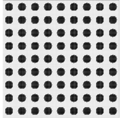
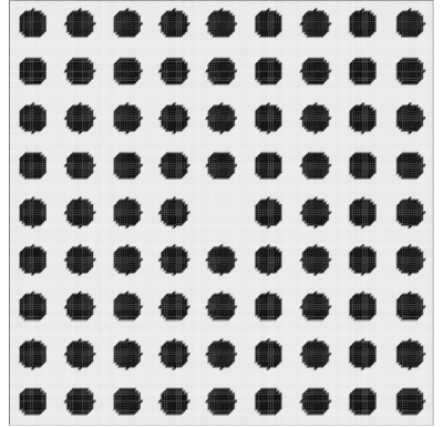
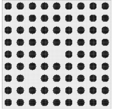
A setting with zero, one and two defects is shown in Figure 1 in the two-dimensional case of a reference material $A_{per}$ consisting of a periodic lattice of circular inclusions.

Figure 1: From left to right: zero defect, one defect and two defects.

Remark 5.

It is illustrative to consider the particular case where the random variable $B_{\eta}$ has a Bernoulli law. This is the case treated in [2]. Then, expansion (3.4) holds exactly with $d\bar{P}_{1}=\delta_{1}-\delta_{0}$. The distribution $d\bar{P}_{2}$ and all other terms of higher order identically vanish. The expressions (3.25) and (3.29) then coincide with (3.17) and (3.18) in [2].

In the next section we prove that $A_{1}^{*,N}$ converges to a finite limit when $N\rightarrow\infty$. The case of the second-order term $A_{2}^{*,N}$, which is shown to be a bounded sequence and thus to converge up to extraction, is discussed in Section 3.4.

3.3 Convergence of the first-order term

We study here the convergence as $N$ goes to infinity of $A_{1}^{*,N}$ defined by (3.25).

Proposition 7.

The sequence $A_{1}^{*,N}$ converges in $\mathbb{R}^{d\times d}$ to a finite limit $\bar{A_{1}^{*}}$ when $N\rightarrow\infty$.

Proof.

We fix $(i,j)\in\llbracket 1,d\rrbracket^{2}$ and study the convergence of $A_{1}^{*,N}e_{i}\cdot e_{j}$.

Using (3.24) and the adjoint problems defined by (2.18), we first obtain, for all
$s\in[-M,M]$,

$$\int_{I_{N}}A_{1}^{s,0}(\nabla w_{i}^{1,s,0,N}+e_{i})\cdot e_{j}=\int_{I_{N}}A_{1}^{s,0}(\nabla w_{i}^{1,s,0,N}+e_{i})\cdot(e_{j}+\nabla\tilde{w}_{j}^{0}).$$

Then, letting the distribution $d\bar{P}_{1}$ act on the left and right-hand sides, and using (3.25), we find that

$$A_{1}^{*,N}e_{i}\cdot e_{j}=\left\langle d\bar{P}_{1}(s),\int_{I_{N}}A_{1}^{s,0}(\nabla w_{i}^{1,s,0,N}+e_{i})\cdot(e_{j}+\nabla\tilde{w}_{j}^{0})\right\rangle.$$ (3.30)

Because of the definition of $A_{1}^{s,0}$,

$$\begin{aligned} \int_{I_{N}}A_{1}^{s,0}(\nabla w_{i}^{1,s,0,N}+e_{i})\cdot(e_{j}+\nabla\tilde{w}_{j}^{0})=\int_{I_{N}}A_{per}(\nabla w_{i}^{1,s,0,N}+e_{i})\cdot(e_{j}+\nabla\tilde{w}_{j}^{0})\\ +\int_{Q}sC_{per}(\nabla w_{i}^{1,s,0,N}+e_{i})\cdot(e_{j}+\nabla\tilde{w}_{j}^{0}).\end{aligned}$$ (3.31)

Next, using (2.18),

$$\begin{aligned} \int_{I_{N}}A_{per}(\nabla w_{i}^{1,s,0,N}+e_{i})\cdot(e_{j}+\nabla\tilde{w}_{j}^{0})&=\int_{I_{N}}(\nabla w_{i}^{1,s,0,N}+e_{i})\cdot A_{per}^{T}(e_{j}+\nabla\tilde{w}_{j}^{0})\\ &=\int_{I_{N}}e_{i}\cdot A_{per}^{T}(e_{j}+\nabla\tilde{w}_{j}^{0}).\end{aligned}$$ (3.32)

We know from Lemma 6 that $\langle d\bar{P}_{1},1\rangle=0$. Thus

$$\left\langle d\bar{P}_{1}(s),\int_{I_{N}}e_{i}\cdot A_{per}^{T}(e_{j}+\nabla\tilde{w}_{j}^{0})\right\rangle=0.$$ (3.33)

Collecting (3.30), (3.31), (3.32) and (3.33), we get

$$A_{1}^{*,N}e_{i}\cdot e_{j}=\left\langle d\bar{P}_{1}(s),\int_{Q}sC_{per}(\nabla w_{i}^{1,s,0,N}+e_{i})\cdot(e_{j}+\nabla\tilde{w}_{j}^{0})\right\rangle.$$ (3.34)

We now define

$$q_{i}^{1,s,0,N}=w_{i}^{1,s,0,N}-w_{i}^{0}.$$ (3.35)

$q_{i}^{1,s,0,N}$ solves

$$\left\{\begin{aligned} &-\mathrm{div}\left(A_{1}^{s,0}\nabla q_{i}^{1,s,0,N}\right)=\mathrm{div}(s\mathds{1}_{Q}C_{per}(\nabla w_{i}^{0}+e_{i}))\quad\mathrm{in}\;I_{N},\\ &q_{i}^{1,s,0,N}\;(N\mathbb{Z})^{d}-\mathrm{periodic}.\end{aligned}\right.$$ (3.36)

Using (3.35) in (3.34), we rewrite

$$A_{1}^{*,N}e_{i}\cdot e_{j} = \left\langle sd\bar{P}_{1}(s),\int_{Q}C_{per}(\nabla w_{i}^{0}+e_{i})\cdot(e_{j}+\nabla\tilde{w}_{j}^{0})\right\rangle$$ (3.37)

$$\qquad+\left\langle d\bar{P}_{1}(s),\int_{Q}sC_{per}(\nabla q_{i}^{1,s,0,N}+e_{i})\cdot(e_{j}+\nabla\tilde{w}_{j}^{0})\right\rangle.$$

The rest of the proof consists in showing that

$$\left\langle d\bar{P}_{1}(s),\int_{Q}sC_{per}(\nabla q_{i}^{1,s,0,N}+e_{i})\cdot(e_{j}+\nabla\tilde{w}_{j}^{0})\right\rangle,$$

which is of course equal to

$$\left\langle sd\bar{P}_{1}(s),\int_{Q}C_{per}(\nabla q_{i}^{1,s,0,N}+e_{i})\cdot(e_{j}+\nabla\tilde{w}_{j}^{0})\right\rangle,$$

converges to a finite limit when $N\rightarrow\infty$.

More precisely, defining

$$\forall s\in[-M,M],\;\forall N\in 2\mathbb{N}+1,\;\;f^{N}(s)=\int_{Q}C_{per}(\nabla q_{i}^{1,s,0,N}+e_{i})\cdot(e_{j}+\nabla\tilde{w}_{j}^{0}),$$

we will prove that the sequence $f^{N}$ and its derivatives converge uniformly, when $N$ goes to infinity, to a limit function $f^{\infty}$ and its derivatives.

Applying Lemma 15 of the appendix to (3.36), we obtain that for all $s\in[-M,M]$, $\nabla q_{i}^{1,s,0,N}$ converges in $L^{2}(Q)$, when $N\rightarrow\infty$, to $\nabla q_{i}^{1,s,0,\infty}$, where $q_{i}^{1,s,0,\infty}$ is a $L^{2}_{loc}(\mathbb{R}^{d})$ function solving

$$\left\{\begin{aligned} &-\mathrm{div}\left(A_{1}^{s,0}\nabla q_{i}^{1,s,0,\infty}\right)=\mathrm{div}(s\mathds{1}_{Q}C_{per}(\nabla w_{i}^{0}+e_{i}))\quad\mathrm{in}\;\mathbb{R}^{d},\\ &\nabla q_{i}^{1,s,0,\infty}\in L^{2}(\mathbb{R}^{d}).\end{aligned}\right.$$ (3.38)

Moreover, arguing as in the proof of Lemma 15 (given in our previous work [2]), it is easy to see that for all $k\in\mathbb{N}$ and all $s\in[-M,M]$, $\nabla\partial_{s}^{k}q_{i}^{1,s,0,N}$ converges in $L^{2}(Q)$ to $\nabla\partial_{s}^{k}q_{i}^{1,s,0,\infty}$.

We then define $f^{\infty}$ by

$$\forall s\in[-M,M],\;\;f^{\infty}(s)=\int_{Q}C_{per}(\nabla q_{i}^{1,s,0,\infty}+e_{i})\cdot(e_{j}+\nabla\tilde{w}_{j}^{0}).$$

Because of (5.4) and (5.5) in Lemma 16 of the appendix, and using a classical result of differentiation under the integral sign, it is clear that

$$\forall k\in\mathbb{N},\forall s\in]-M,M[,\;\frac{d^{k}}{ds^{k}}f^{N}(s)=\int_{Q}C_{per}(\nabla\partial^{k}_{s}q_{i}^{1,s,0,N}+e_{i})\cdot(e_{j}+\nabla\tilde{w}_{j}^{0}),$$

and

$$\forall k\in\mathbb{N},\forall s\in]-M,M[,\;\frac{d^{k}}{ds^{k}}f^{\infty}(s)=\int_{Q}C_{per}(\nabla\partial^{k}_{s}q_{i}^{1,s,0,\infty}+e_{i})\cdot(e_{j}+\nabla\tilde{w}_{j}^{0}).$$

The convergence of $\nabla\partial_{s}^{k}q_{i}^{1,s,0,N}$ to $\nabla\partial_{s}^{k}q_{i}^{1,s,0,\infty}$ in $L^{2}(Q)$ for every $k\in\mathbb{N}$ thus yields

$$\forall k\in\mathbb{N},\forall s\in]-M,M[,\lim_{N\rightarrow+\infty}\frac{d^{k}}{ds^{k}}f^{N}(s)=\frac{d^{k}}{ds^{k}}f^{\infty}(s).$$ (3.39)

On the other hand, we deduce from Lemma 17 that there exists a constant $C(p_{1},M)$ (recall that $p_{1}$ is the order of $d\bar{P}_{1}(s)$) such that for all $k\in\llbracket 0,p_{1}\rrbracket$,

$$\forall(s,s^{\prime})\in]-M,M[^{2},\forall N\in 2\mathbb{N}+1,\;\;|\frac{d^{k}}{ds^{k}}f^{N}(s)-\frac{d^{k}}{ds^{k}}f^{N}(s^{\prime})|\leq C(p_{1},M)|s-s^{\prime}|.$$ (3.40)

It is straightforward to see that (3.39) and (3.40) imply that

$$\forall 0\leq k\leq p_{1},\;\frac{d^{k}}{ds^{k}}f^{N}\mathrm{\;converges\;uniformly\;to\;}\frac{d^{k}}{ds^{k}}f^{\infty}\;\mathrm{\;in\;}]-M,M[.$$ (3.41)

It follows from (3.5) and (3.41) that

$$\langle sd\bar{P}_{1}(s),f^{N}(s)\rangle\rightarrow\langle sd\bar{P}_{1}(s),f^{\infty}(s)\rangle,$$

and then

$$\begin{aligned} &\left\langle d\bar{P}_{1}(s),\int_{Q}sC_{per}(\nabla q_{i}^{1,s,0,N}+e_{i})\cdot(e_{j}+\nabla\tilde{w}_{j}^{0})\right\rangle\\ &\qquad\qquad\underset{N\rightarrow\infty}{\rightarrow}\left\langle d\bar{P}_{1}(s),\int_{Q}sC_{per}(\nabla q_{i}^{1,s,0,\infty}+e_{i})\cdot(e_{j}+\nabla\tilde{w}_{j}^{0})\right\rangle.\end{aligned}$$ (3.42)

Collecting (3.37) and (LABEL:convdp1), we conclude that $A_{1}^{*,N}$ converges to a limit tensor $\bar{A_{1}^{*}}$ defined by

$$\begin{aligned} \forall(i,j)\in\llbracket 1,d\rrbracket^{2},\;\;\bar{A_{1}^{*}}e_{i}\cdot e_{j}&=\left\langle sd\bar{P}_{1}(s),\int_{Q}C_{per}\left(\nabla w_{i}^{0}+e_{i}\right)\cdot(e_{j}+\nabla\tilde{w}_{j}^{0})\right\rangle\\ &+\left\langle d\bar{P}_{1}(s),\int_{Q}sC_{per}\left(\nabla q_{i}^{1,s,0,\infty}+e_{i}\right)\cdot(e_{j}+\nabla\tilde{w}_{j}^{0})\right\rangle.\end{aligned}$$ (3.43)

∎

3.4 Second-order term

For completeness, we state here the result concerning the second-order term $A_{2}^{*,N}$ in (3.19), proved in [1]:

Proposition 8.

The sequence $A_{2}^{*,N}$ defined by (3.29) is bounded in $\mathbb{R}^{d\times d}$ and therefore converges up to extraction.

We firmly believe that $A_{2}^{*,N}$ is actually a convergent sequence, as shown by our numerical tests thereafter. We also stress that the explicit computations of Section 5.3 prove this convergence in dimension one.

4 Numerical experiments

The purpose of this section is to assess the numerical relevance of the approaches of Sections 2 and 3. To this end we build and homogenize stochastic composite materials using laws that satisfy the assumptions of these sections. Our motivations are not strictly identical for the two approaches. In contrast to the first approach which relies on a rigorous proof, our second approach is formal and we thus need to demonstrate its correctness experimentally (note that the tests performed in [2] in the Bernoulli case are already to be considered as a component of the validation of the approach). We wish to check that the expansions derived in Sections 2 and 3 provide an accurate and efficient approximation to the direct stochastic computation. The limited computational facilities we have access to impose that we restrict ourselves to the two-dimensional setting. We first explain our general methodology, which is the same as that presented in [2], and then make precise the specific settings.

4.1 Methodology

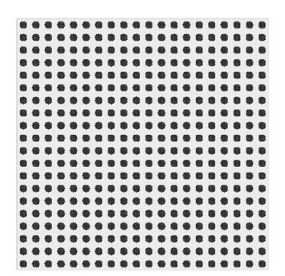
We mainly consider as in [2] a reference material $A_{per}$ that consists of a constant background reinforced by a periodic lattice of circular inclusions, that is

$$A_{per}(x_{1},x_{2})=20\times Id+100\sum_{k\in\mathbb{Z}^{2}}\mathds{1}_{B(k,0.3)}(x_{1},x_{2})\times Id,$$

where $B(k,0.3)$ is the ball of center $k$ and radius $1$. Loosely speaking, the role of the perturbation is to randomly eliminate some fibers:

$$C_{per}(x_{1},x_{2})=-100\sum_{k\in\mathbb{Z}^{d}}\mathds{1}_{B(k,0.3)}(x_{1},x_{2})\times Id.$$

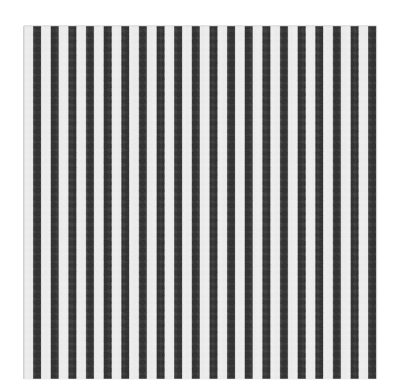
We will also, in our last test, consider a laminate

$$A_{per}(x_{1},x_{2})=5+10\sum_{l\in\mathbb{Z}}\mathds{1}_{l\leq x_{1}\leq l+1}(x_{1},x_{2}),$$

with the perturbation yielding an error in the lamination direction:

$$C_{per}(x_{1},x_{2})=10\sum_{l\in\mathbb{Z}}\mathds{1}_{l\leq x_{2}\leq l+1}(x_{1},x_{2})\times Id-10\sum_{l\in\mathbb{Z}}\mathds{1}_{l\leq x_{1}\leq l+1}(x_{1},x_{2})\times Id.$$

For both materials (shown in Figure 2), we have chosen the values of the coefficients in order to have a high contrast between $A_{per}$ and $A_{per}+C_{per}$ and thus for the perturbation to have an important impact on the microscopic structure. The specific value of these coefficients has no other significance.

We will consider different perturbations $b_{\eta}$, all of which satisfy (3.1) with the $B_{\eta}^{k}$ independent and identically distributed.

Figure 2: Left: a periodic lattice of circular inclusions. Right: a one-dimensional laminate.

Our goal is to compare $A_{\eta}^{*}$ with its approximation $A_{per}^{*}+\eta A_{1}^{*,N}+\eta^{2}A_{2}^{*,N}$. A major computational difficulty is the computation of the “exact” matrix $A_{\eta}^{*}$ given by formula (2.9). It ideally requires to solve the stochastic cell problems (2.8) on $\mathbb{R}^{d}$. To this end we first use ergodicity and formula (3.11), and actually compute, for a given realization $\omega$ and a domain $I_{N}$ chosen here to be $[0,N]^{2}$ for convenience, $A_{\eta}^{*,N}(\omega)$ defined by

$$A_{\eta}^{*,N}(\omega)e_{i}=\frac{1}{N^{d}}\int_{I_{N}}A_{\eta}(x,\omega)(\nabla w_{i}^{\eta,N,\omega}(x)+e_{i})dx.$$ (4.1)

In a second step, we take averages over the realizations $\omega$.

For each $\omega$, we use the finite element software FreeFem++ (available at www.freefem.org) to solve the boundary value problems (3.10) and compute the integrals (4.1). We work with standard P1 finite elements on a triangular mesh such that there are $10$ degrees of freedom on each edge of the unit cell $Q$.

We define an approximate value $A_{\eta}^{*,N}$ as the average of $A_{\eta}^{*,N}(\omega)$ over $40$ realizations $\omega$. Our numerical experiments indeed show that the number $40$ is sufficiently large for the convergence of the Monte-Carlo computation. We then let $N$ grow from $5$ to $80$ by steps of $5$. We observe that $A_{\eta}^{*,N}$ stabilizes at a fixed value around $N=80$ and thus take $A_{\eta}^{*,80}$ as the reference value for $A_{\eta}^{*}$ in our subsequent tests.

The next step is to compute the zero-order term $A_{per}^{*}$, and the first-order and second-order deterministic corrections. Using the same mesh and finite elements as for our reference computation above, we compute $A_{per}^{*}$ using (2.10) and (2.11). The computation of the next orders depends on the setting:

• in the setting of Section $2$, the first-order correction is given by (2.15) in Theorem 2 and is thus independent of $N$; since $b_{\eta}$ is of the form (2.26), we use formula (2.30) in Corollary 4 for the second-order correction which depends on $N$ through the term $t_{i}$ defined on $\mathbb{R}^{d}$ by (2.31), and which has to be approximated on $I_{N}$; we let $N$ grow from $5$ to $80$ by steps of $5$;

• in the setting of Section $3$, the corrections $A_{1}^{*,N}$ and $A_{2}^{*,N}$ are respectively given by (3.25) and (3.29); we let $N$ grow from $5$ to $80$ by steps of $5$ for $A_{1}^{*,N}$; the computation of $A_{2}^{*,N}$ being far more expensive (there is not only an integral over $I_{N}$ but also a sum over the $N^{2}$ cells in (3.29)), we have to limit ourselves to $N=25$ and approximate the value for $N$ larger than $25$ by the value obtained for $N=25$.

We stress that there are three distinct sources of error in these computations:

• the finite elements discretization error;

• the truncation error due to the replacement of $\mathbb{R}^{d}$ with $I_{N}$, in the computation of the stochastic cell problems (2.8) that are replaced with (3.10), as well as in the computation of the integrals (4.1);

• the stochastic error arising from the approximation of the expectation value by an empirical mean.

Detailed comments on these various errors and the way we deal with them are provided in [2]. We just emphasize, in the setting of Section 3, that it is not our purpose to prove through our tests that

$$A_{\eta}^{*}=A_{per}^{*}+\eta\bar{A_{1}^{*}}+\eta^{2}\bar{A_{2}^{*}}+o(\eta^{2})$$

with a $o(\eta^{2})$ which would be independent of $N$, of the number of realizations and of the size of the mesh. We only wish to demonstrate that the second-order expansion is an approximation to $A_{\eta}^{*}$ sufficiently good for all practical purposes. We will observe that $A_{2}^{*,N}$ is not only bounded as stated in Proposition 8 but converges to a limit $\bar{A_{2}^{*}}$, and that both $A_{1}^{*,N}$ and $A_{2}^{*,N}$ converge to their respective limits faster than $A_{\eta}^{*,N}$ to $A_{\eta}^{*}$ (which is expected since the former quantities are deterministic and contain less information). We will also observe that $A_{per}^{*}+\eta A_{1}^{*,N}$ is closer to $A_{\eta}^{*}$ than $A_{per}^{*}$ and that the inclusion of the second order improves the situation for $A_{per}^{*}+\eta A_{1}^{*,N}+\eta^{2}A_{2}^{*,N}$ is even closer.

To present our numerical results, we choose the first diagonal entry $(1,1)$ of all the matrices considered. Other coefficients in the matrices behave qualitatively similarly. We illustrate a practical interval of confidence for our Monte-Carlo computation of $A_{\eta}^{*}$ by showing, for each $N$, the minimum and maximum values of $A_{\eta}^{*,N}(\omega)$ achieved over the $40$ realizations $\omega$.

We will use the following legend in the graphs:

• periodic: gives the value of the periodic homogenized tensor $A_{per}^{*}$;

• first-order: gives the value of the first-order expansion;

• second-order: gives the value of the second-order expansion;

• stochastic mean, minima and maxima: respectively give the values of $A_{\eta}^{*,N}$ and the extrema obtained in the computation of the empirical mean.
  

Finally, the results are given for various values of $\eta$ which serve the purpose of testing our approach in a diversity of situations, and in particular for perturbations that are “not so small”.

4.2 An example of setting for our theory in Section 2 (and 3)

Consider $B_{\eta}=\eta\,G\,\mathds{1}_{0\leq\eta G\leq 1}$ where $G$ is a normalized centered Gaussian random variable. It is easy to check that

$$B_{\eta}=\eta G\mathds{1}_{0\leq G\leq+\infty}+o(\eta^{2})\quad\mathrm{in\;}L^{2}(\Omega),$$

so that Corollary 4 of Section 2 applies. Alternatively, we can use Lemma 5, which gives

$$dP_{\eta} = \delta_{0}-\eta\frac{1}{\sqrt{2}}\delta_{0}^{\prime}+\frac{\eta^{2}}{4}\delta_{0}^{\prime\prime}+o(\eta^{2})\;\mathrm{in}\;\mathcal{E}^{\prime}(\mathbb{R}),$$

to perform our formal approach. We verify in Section 5.4 of the appendix that both approaches yield the same results up to second order.

We show results for the lattice of inclusions and for $\eta=0.1$ and $\eta=0.2$ (Figures 3 and 4 respectively).

Figure 3: Inclusions - results for a Gaussian perturbation and $\eta=0.1$. Above: complete results. Below: close-up on $A_{\eta}^{*,N}$ and the first and second-order corrections.

Figure 4: Inclusions - Results for a Gaussian perturbation and $\eta=0.2$. Above: complete results. Below: close-up on $A_{\eta}^{*,N}$ and the first and second-order corrections.

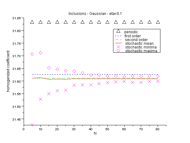
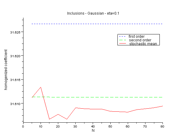
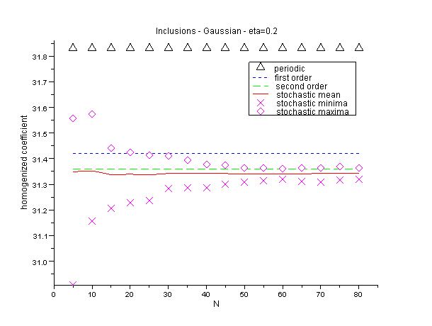
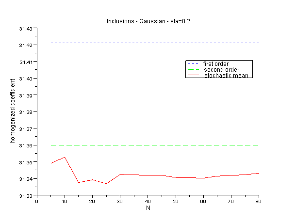
The results are very satisfying for both values of $\eta$. The first-order correction, which does not depend on $N$, enables to get substantially closer to $A_{\eta}^{*}$. Moreover, it is clear (especially from the close-ups) that the second-order correction $A_{2}^{*,N}$ converges very fast (convergence is already reached at $N=5$), and in particular much faster than the stochastic computation $A_{\eta}^{*,N}$. It also provides excellent accuracy.

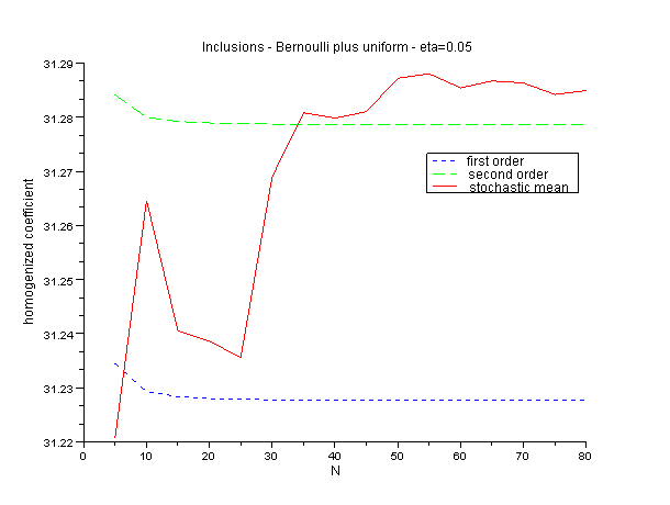
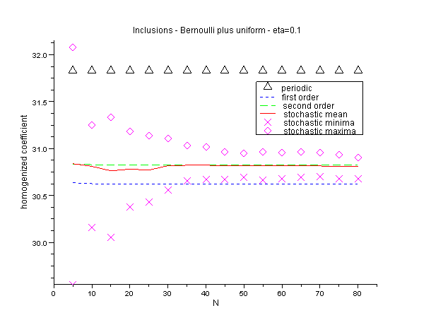
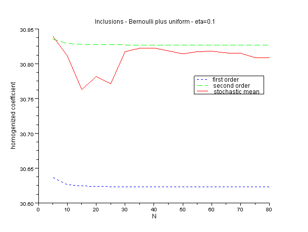
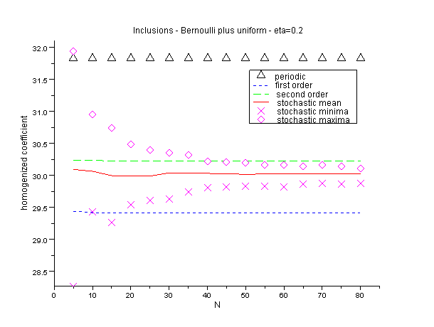
4.3 A first example of setting for our formal approach of Section 3

Consider $R_{\eta}$ a random variable having Bernoulli law with parameter $\eta$, and $G$ a normalized centered Gaussian random variable independent of $R_{\eta}$. We define the product random variable $B_{\eta}=R_{\eta}\times\eta G\mathds{1}_{|\eta G|\leq 1}$. Then

$$\mathbb{E}(\varphi(B_{\eta})) = \mathbb{E}(\varphi(R_{\eta}\times\eta G\mathds{1}_{|\eta G|\leq 1}))$$

$$= \eta\mathbb{E}(\varphi(\eta G\mathds{1}_{|\eta G|\leq 1}))+(1-\eta)\varphi(0)$$

$$= \eta(\varphi(0)+\eta\mathbb{E}(G)\varphi^{\prime}(0)+\frac{\eta^{2}}{2}\varphi^{\prime\prime}(0)+o(\eta^{2}))+(1-\eta)\varphi(0)$$

$$= \varphi(0)+\frac{\eta^{3}}{2}\varphi^{\prime\prime}(0)+o(\eta^{3}).$$

This implies

$$dP_{\eta}=\delta_{0}+\frac{\eta^{3}}{2}\delta^{{}^{\prime\prime}}_{0}+o(\eta^{3})\quad\mathrm{in\;}\mathcal{E}^{\prime}(\mathbb{R}).$$ (4.2)

In this case we only consider the first-order correction since the dominant order in (4.2) is already tiny. We present the results in the case of the lattice of inclusions, for $\eta=0.2$, $\eta=0.3$ and $\eta=0.5$ (Figures 5, 6, 7 respectively).

Figure 5: Inclusions - results for perturbation (4.2) and $\eta=0.1$. Above: complete results. Below: close-up on $A_{\eta}^{*,N}$ and the first-order correction.

Figure 6: Inclusions - results for perturbation (4.2) and $\eta=0.3$. Above: complete results. Below: close-up on $A_{\eta}^{*,N}$ and the first-order correction.

Figure 7: Inclusions - results for perturbation (4.2) and $\eta=0.5$. Above: complete results. Below: close-up on $A_{\eta}^{*,N}$ and the first-order correction.

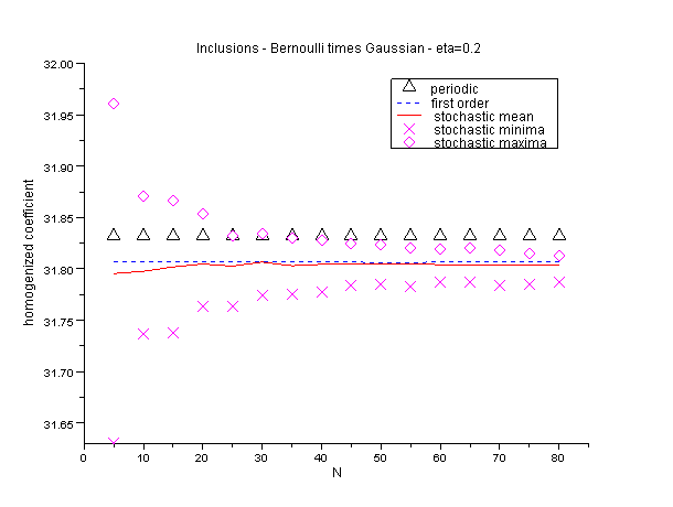
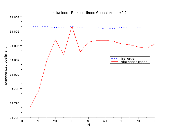
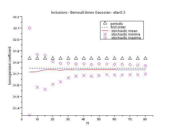
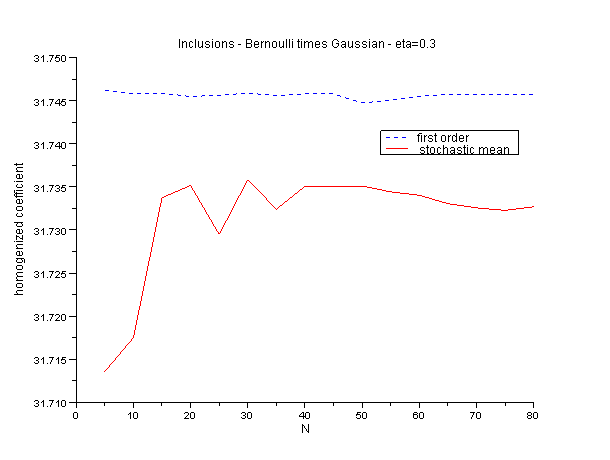
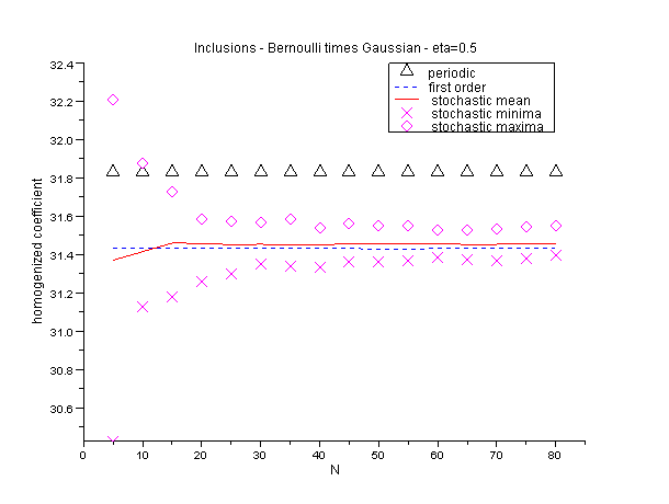
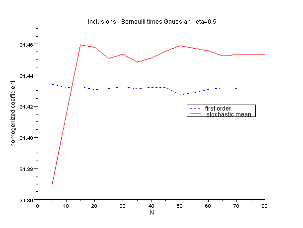
Once again, our approach converges rapidly and allows for an accurate approximate value of $A_{\eta}^{*}$ even for $\eta$ as large as 0.5.

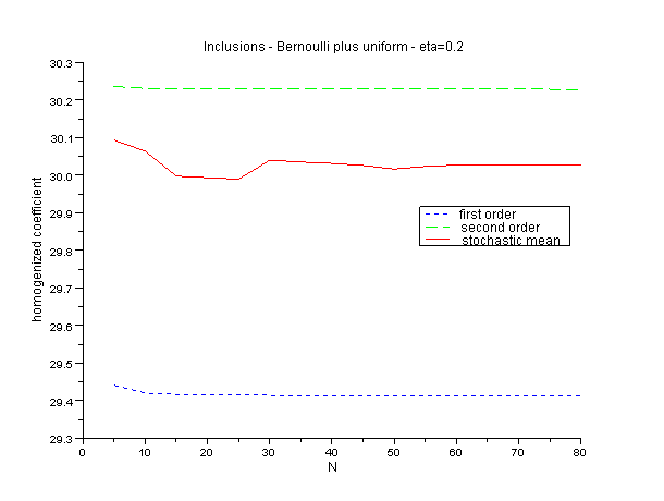
4.4 A second example of setting for our formal approach of Section 3

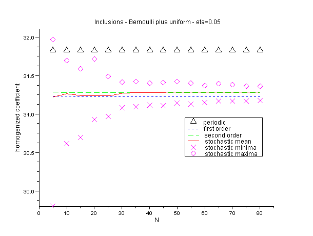
Consider $R_{\eta}$ a random variable having Bernoulli law with parameter $\eta$, and $U$ a uniform variable on $[0,1]$ independent of $R_{\eta}$. We define $B_{\eta}=R_{\eta}-\eta U$. Then

$$\mathbb{E}(\varphi(B_{\eta})) = \mathbb{E}(\varphi(R_{\eta}-\eta U))$$

$$= \eta\mathbb{E}(\varphi(1-\eta U))+(1-\eta)\mathbb{E}(\varphi(-\eta U))$$

$$= \eta\left(\varphi(1)-\eta\mathbb{E}(U)\varphi^{\prime}(1)+o(\eta)\right)$$

$$+(1-\eta)\left(\varphi(0)-\eta\mathbb{E}(U)\varphi^{\prime}(0)+\frac{\eta^{2}}{2}\mathbb{E}(U^{2})\varphi^{\prime\prime}(0)+o(\eta^{2})\right)$$

$$= \varphi(0)+\eta\left(-\mathbb{E}(U)\varphi^{\prime}(0)+\varphi(1)-\varphi(0)\right)$$

$$+\eta^{2}\left(-\mathbb{E}(U)(\varphi^{\prime}(1)-\varphi^{\prime}(0))+\frac{1}{2}\mathbb{E}(U^{2})\varphi^{\prime\prime}(0)\right)+o(\eta^{2}),$$

so that

$$\begin{aligned} dP_{\eta}=&\delta_{0}+\eta\left(-\mathbb{E}(U)\delta^{\prime}_{0}+\delta_{1}-\delta_{0}\right)\\ &+\eta^{2}\left(-\mathbb{E}(U)(\delta^{\prime}_{1}-\delta^{\prime}_{0})+\frac{1}{2}\mathbb{E}(U^{2})\delta^{\prime\prime}(0)\right)+o(\eta^{2})\quad\mathrm{in\;}\mathcal{E}^{\prime}(\mathbb{R}).\end{aligned}$$ (4.3)

Notice that this complex case is a mixture of Sections 2 and 3. The first-order perturbation is of course only the sum of the first-order perturbations for a Bernoulli law (Section 3 and [2]) and a uniform law (Section 2). The interaction of these laws at order 2, and notably the $\delta^{\prime}_{1}$ term, is much more involved and requires the computation of the cross derivatives of $w_{i}^{2,s,t,0,k,N}$ with respect to $s$ and $t$ at $s=0$ and $t=1$.

We give the results in the case of the inclusions and for $\eta=0.05$, $\eta=0.1$ and $\eta=0.2$ (Figures 8, 9, 10, respectively).

For $\eta=0.05$ and $\eta=0.1$, the results display the same features as in our previous tests and are very good. The case $\eta=0.2$ is instructive: the second-order expansion significantly departs from the "exact" value provided by the direct stochastic computation. Our interpretation is that, far from contradicting the validity of our expansion in the limit of small $\eta$, it shows the limitations of the approach. The value $\eta=0.2$ is too large for the expansion to be accurate in the case of a lattice of inclusions with a high contrast between the inclusions and the surrounding phase.

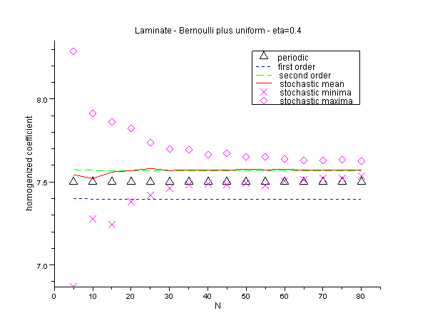
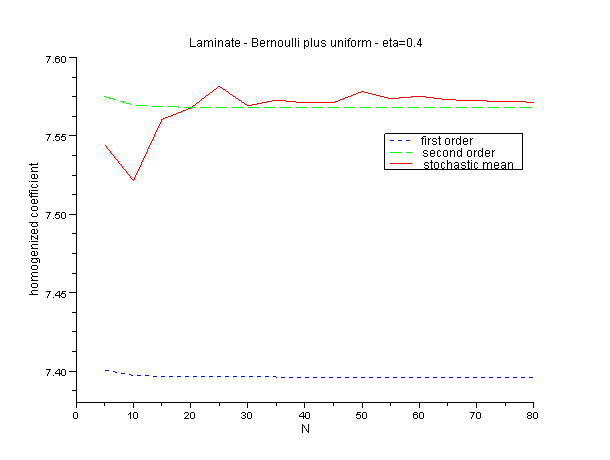
Interestingly, a value of $\eta$ twice as large (0.4) provides a very accurate approximation for another material, as shown by our final test performed on the laminate (Figure 11).

Our approach has limitations and deteriorates, like any asymptotic approach, for large values of $\eta$. The threshold is case dependent. The approach is however generically robust.

Figure 8: Inclusions- results for perturbation (4.3) and $\eta=0.05$. Above: complete results. Below: close-up on $A_{\eta}^{*,N}$ and the first and second-order corrections.

Figure 9: Inclusions - results for perturbation (4.3) and $\eta=0.1$. Above: complete results. Below: close-up on $A_{\eta}^{*,N}$ and the first and second-order corrections.

Figure 10: Inclusions - results for perturbation (4.3) and $\eta=0.2$. Above: complete results. Below: close-up on $A_{\eta}^{*,N}$ and the first and second-order corrections.

Figure 11: Laminate - results for perturbation (4.3) and $\eta=0.4$. Above: complete results. Below: close-up on $A_{\eta}^{*,N}$ and the first and second-order corrections.

5 Appendix

The objectives of this appendix are diverse. We first quickly recall some elements of distribution theory. We then prove technical results used in Section 3. Next we show that the approach formally derived in Section 3 is rigorous in dimension one. Finally we prove that this approach is also rigorous, in general dimensions, in a specific setting close to that of Theorem 2 and Corollary 4.

5.1 Elements of distribution theory

We recall here some basic definitions and results of distribution theory for convenience of the reader. See [6] for a comprehensive presentation.

In this section $\mathcal{O}$ denotes an open set in $\mathbb{R}$.

Definition 9.

We denote by $\mathcal{D}(\mathcal{O})$ the space of infinitely differentiable functions on $\mathcal{O}$ having compact support in $\mathcal{O}$.

Definition 10.

T is a distribution on $\mathcal{O}$ if $T$ is a linear form on $\mathcal{D}(\mathcal{O})$ satisfying the following continuity property: for every compact $K\subset\mathcal{O}$, there exists an integer $p$ and a constant $C$ such that for all $\varphi\in\mathcal{D}(\mathcal{O})$ having compact support in $K$,

$$|\langle T,\varphi\rangle|\leq C\sup_{x\in K,0\leq n\leq p}\left|\frac{d^{n}}{dx^{n}}\varphi(x)\right|.$$ (5.1)

The space of distributions on $\mathcal{O}$ is denoted by $\mathcal{D}^{\prime}(\mathcal{O})$.

If the integer $p$ in (5.1) can be chosen independently of $K$, the distribution $T$ is said to have a finite order. The smallest possible value for $p$ is called the order of $T$.

Definition 11.

A distribution $T\in\mathcal{D}^{\prime}(\mathcal{O})$ is said to have compact support if there exists a compact set $K\subset\mathcal{O}$ such that for all $\varphi\in\mathcal{D}(\mathcal{O})$ having compact support in $\mathcal{O}\backslash K$, $\langle T,\varphi\rangle=0$.

The support of $T$ is defined as the smallest compact set $K$ which satisfies the above assertion.

The space of distributions on $\mathcal{O}$ having compact support is denoted by $\mathcal{E}^{\prime}(\mathcal{O})$.

Proposition 12.

If $T\in\mathcal{E}^{\prime}(\mathcal{O})$, its action on $\mathcal{D}(\mathcal{O})$ can be naturally extended to $\mathcal{C}^{\infty}(\mathcal{O})$. Denoting by $K$ a compact neighborhood of the support of $T$, and by $\chi$ a cut-off function in $\mathcal{D}(\mathcal{O})$ equal to 1 on the support of $T$ and vanishing on $\mathcal{O}\backslash K$, we define

$$\forall\varphi\in\mathcal{C}^{\infty}(\mathcal{O}),\;\langle T,\varphi\rangle:=\langle T,\chi\varphi\rangle.$$

This definition does not depend on $K$ and $\chi$.

Proposition 13.

If a distribution $T$ is in $\mathcal{E}^{\prime}(\mathcal{O})$, it has a finite order. Denoting by $p$ its order and by $K$ a compact neighborhood of the support of $T$, there exists a constant $C>0$ such that:

$$\forall\varphi\in C^{\infty}(\mathcal{O}),\;|\langle T,\varphi\rangle|\leq C\sup_{x\in K,0\leq n\leq p}\left|\frac{d^{n}}{dx^{n}}\varphi(x)\right|.$$

5.2 Some technical results

This section is devoted to the proof of technical lemmas used in Section 3. Loosely speaking, these lemmas all deal with the variation of the supercell correctors defined by (3.15), (3.24), and (3.28) with respect to the amplitudes of the defects.

Lemma 14.

Let $\tilde{H}^{1}_{per}(I_{N})$ be the set of $(N\mathbb{Z})^{d}$-periodic functions in $H^{1}_{loc}(\mathbb{R}^{d})$ with zero mean on $I_{N}$. The function

$$F:(s_{1},\cdots,s_{N^{d}})\in]-M,M[^{N^{d}}\mapsto\bar{w}_{i}^{s_{1},\cdots,s_{N^{d}}}\in\tilde{H}^{1}_{per}(I_{N}),$$

where $\bar{w}_{i}^{s_{1},\cdots,s_{N^{d}}}=w_{i}^{s_{1},\cdots,s_{N^{d}}}-\int_{I_{N}}w_{i}^{s_{1},\cdots,s_{N^{d}}}$ and $w_{i}^{s_{1},\cdots,s_{N^{d}}}$ is defined by (3.15), is $C^{\infty}$.

Proof.

For $(s_{1},\cdots,s_{N^{d}})\in[-M,M]^{N^{d}}$, $\bar{w}_{i}^{s_{1},\cdots,s_{N^{d}}}$ is the unique solution to

$$\left\{\begin{aligned} &-\mathrm{div}\left(A^{s_{1},\cdots,s_{N^{d}}}(\nabla\bar{w}_{i}^{s_{1},\cdots,s_{N^{d}}}+e_{i})\right)=0\quad\,\mathrm{in}\,I_{N},\\ &\bar{w}_{i}^{s_{1},\cdots,s_{N^{d}}}\,(N\mathbb{Z})^{d}-\mathrm{periodic},\quad\int_{I_{N}}\bar{w}_{i}^{s_{1},\cdots,s_{N^{d}}}=0,\end{aligned}\right.$$

so that $F$ is well defined.

Let us now define $G:]-M,M[^{N^{d}}\times\tilde{H}^{1}_{per}(I_{N})\rightarrow H^{-1}(I_{N})$ by

$$G(s_{1},\cdots,s_{N^{d}},w)=-\mathrm{div}\left(A^{s_{1},\cdots,s_{N^{d}}}(\nabla w+e_{i})\right),$$

so that $F(s_{1},\cdots,s_{N^{d}})=\bar{w}_{i}^{s_{1},\cdots,s_{N^{d}}}$ is the unique solution to

$$G(s_{1},\cdots,s_{N^{d}},F(s_{1},\cdots,s_{N^{d}}))=0.$$

It is easy to see that $G$ is a $C^{1}$ function, and that

$$\forall h\in\tilde{H}^{1}_{per}(I_{N}),\quad\partial_{w}G(s_{1},\cdots,s_{N^{d}},w)\cdot h=-\mathrm{div}\left(A^{s_{1},\cdots,s_{N^{d}}}\nabla h\right),$$

where $\partial_{w}G(s_{1},\cdots,s_{N^{d}},w)$ is the first derivative of $G$ with respect to $w$ at $(s_{1},\cdots,s_{N^{d}},w)$.

The Lax-Milgram theorem and the coercivity of $A^{s_{1},\cdots,s_{N^{d}}}$ show that $\partial_{w}G(s_{1},\cdots,s_{N^{d}},w)$ is an isomorphism. We can therefore apply the inverse function theorem and deduce that $F$ is $C^{1}$, with $\partial_{s_{l}}F$ the unique solution to

$$\left\{\begin{aligned} &-\mathrm{div}\left(A^{s_{1},\cdots,s_{N^{d}}}(\nabla\partial_{s_{l}}F)\right)=\mathrm{div}\left(\mathds{1}_{Q_{l}}C_{per}(\nabla F+e_{i})\right)\quad\,\mathrm{in}\,I_{N},\\ &\partial_{s_{l}}F\,(N\mathbb{Z})^{d}-\mathrm{periodic},\quad\int_{I_{N}}\partial_{s_{l}}F=0.\end{aligned}\right.$$

Arguing by induction, we obtain that $F$ is a $C^{\infty}$ function.

∎

For consistency, we state next a lemma proved in [2, Lemma 6]

Lemma 15.

Consider $f\in L^{2}(Q)$, and a tensor field $A$ from $\mathbb{R}^{d}$ to $\mathbb{R}^{d\times d}$ such that there exist $\lambda>0$ and $\Lambda>0$ such that

$$\forall\xi\in\mathbb{R}^{d},\mathrm{\;a.e\;in\;}x\in\mathbb{R}^{d},\;\lambda|\xi|^{2}\leq A(x)\xi\cdot\xi\;\mathrm{and}\;|A(x)\xi|\leq\Lambda|\xi|.$$

Consider $q^{N}$ solution to

$$\left\{\begin{aligned} &-\mathrm{div}\left(A\nabla q^{N}\right)=\mathrm{div}(\mathds{1}_{Q}f)\quad\mathrm{in}\;I_{N},\\ &q^{N}\,(N\mathbb{Z})^{d}-\mathrm{periodic}.\end{aligned}\right.$$ (5.2)

Then $\mathds{1}_{I_{N}}\nabla q^{N}$ converges in $L^{2}(\mathbb{R}^{d})$, when $N$ goes to infinity, to $\nabla q^{\infty}$, where $q^{\infty}$ is a $L^{2}_{loc}(\mathbb{R}^{d})$ function solving

$$\left\{\begin{aligned} &-\mathrm{div}\left(A\nabla q^{\infty}\right)=\mathrm{div}(\mathds{1}_{Q}f)\quad\mathrm{in}\;\mathbb{R}^{d},\\ &\nabla q^{\infty}\in L^{2}(\mathbb{R}^{d}).\end{aligned}\right.$$ (5.3)

Lemma 16.

Consider $q_{i}^{1,s,0,N}$ and $q_{i}^{1,s,0,\infty}$ solutions to (3.36) and (3.38) respectively, and $k\in\mathbb{N}$. There exists a constant $C(k,M)$, such that

$$\forall s\in]-M,M[\,,\;\forall N\in 2\mathbb{N}+1,\;\;\|\nabla\partial_{s}^{k}q_{i}^{1,s,0,N}\|_{L^{2}(I_{N})}\leq C(k,M)\|\nabla w_{i}^{0}+e_{i}\|_{{L^{2}}(Q)},$$ (5.4)

$$\forall s\in]-M,M[\,,\;\;\|\nabla\partial_{s}^{k}q_{i}^{1,s,0,\infty}\|_{L^{2}(\mathbb{R}^{d})}\leq C(k,M)\|\nabla w_{i}^{0}+e_{i}\|_{{L^{2}}(Q)}.$$ (5.5)

Proof.

Multiplying the first line of (3.36) by $q_{i}^{1,s,0,N}$ and integrating by parts, we find that

$$\|\nabla q_{i}^{1,s,0,N}\|_{L^{2}(I_{N})}\leq M\frac{\|C_{per}\|_{L^{\infty}(Q)}}{\alpha}\|\nabla w_{i}^{0}+e_{i}\|_{{L^{2}}(Q)},$$ (5.6)

where $\alpha$ is defined by (2.6).

Thus (5.4) is true for $k=0$ with $C(0,M)=M\frac{\|C_{per}\|_{L^{\infty}(Q)}}{\alpha}$.

Next, the first derivative $\partial_{s}q_{i}^{1,s,0,N}$ is solution to

$$\left\{\begin{aligned} &-\mathrm{div}(A_{1}^{s,0}\nabla\partial_{s}q_{i}^{1,s,0,N})=\mathrm{div}\left(\mathds{1}_{Q}C_{per}(\nabla w_{i}^{0}+e_{i})\right)+\mathrm{div}\left(\mathds{1}_{Q}C_{per}\nabla q_{i}^{1,s,0,N}\right)\quad\mathrm{in}\;I_{N},\\ &\partial_{s}q_{i}^{1,s,0,N}\;\;(N\mathbb{Z})^{d}-\mathrm{periodic},\end{aligned}\right.$$ (5.7)

from which we deduce

$$\|\nabla\partial_{s}q_{i}^{1,s,0,N}\|_{L^{2}(I_{N})}\leq\frac{\|C_{per}\|_{L^{\infty}(Q)}}{\alpha}\left(\|\nabla w_{i}^{0}+e_{i}\|_{{L^{2}}(Q)}+\|\nabla q_{i}^{1,s,0,N}\|_{{L^{2}}(Q)}\right)$$

and, using (5.6),

$$\|\nabla\partial_{s}q_{i}^{1,s,0,N}\|_{L^{2}(I_{N})}\leq\frac{\|C_{per}\|_{L^{\infty}(Q)}}{\alpha}(M+1)\|\nabla w_{i}^{0}+e_{i}\|_{{L^{2}}(Q)}.$$

Thus (5.4) is true for $k=1$ with $C(1,M)=(M+1)\frac{\|C_{per}\|_{L^{\infty}(Q)}}{\alpha}$.

Finally, we have for $k\geq 2$

$$\left\{\begin{aligned} &-\mathrm{div}(A_{1}^{s,0}\nabla\partial_{s}^{k}q_{i}^{1,s,0,N})=k\mathrm{div}\left(\mathds{1}_{Q}C_{per}\nabla\partial_{s}^{k-1}q_{i}^{1,s,0,N}\right)\quad\mathrm{in}\;I_{N},\\ &\nabla\partial_{s}^{k}q_{i}^{1,s,0,N}\;\;(N\mathbb{Z})^{d}-\mathrm{periodic},\end{aligned}\right.$$ (5.8)

so that an easy induction proves (5.4). The proof of (5.5) is identical. ∎

The following result is an immediate consequence of Lemma 16.

Lemma 17.

Consider $q_{i}^{1,s,0,N}$ and $q_{i}^{1,s,0,\infty}$ solutions to (3.36) and (3.38) respectively. For every $k\in\mathbb{N}$, there exists a constant $C(k,M)$ such that for all $(s,s^{\prime})\in]-M,M[^{2}$,

$$\forall N\in 2\mathbb{N}+1,\;\;\|\nabla\partial_{s}^{k}q_{i}^{1,s,0,N}-\nabla\partial_{s}^{k}q_{i}^{1,s^{\prime},0,N}\|_{L^{2}(I_{N})}\leq C(k,M)\|\nabla w_{i}^{0}+e_{i}\|_{{L^{2}}(Q)}|s-s^{\prime}|,$$ (5.9)

$$\|\nabla\partial_{s}^{k}q_{i}^{1,s,0,\infty}-\nabla\partial_{s}^{k}q_{i}^{1,s^{\prime},0,\infty}\|_{L^{2}(\mathbb{R}^{d})}\leq C(k,M)\|\nabla w_{i}^{0}+e_{i}\|_{{L^{2}}(Q)}|s-s^{\prime}|.$$ (5.10)

5.3 The one-dimensional case

We address here the one-dimensional context. All the computations are explicit, for the settings of Sections 2 and 3. To stress the fact that we deal with scalar quantities, we use lower-case letters for the tensors. Note also that in this section $Q=[-\frac{1}{2},\frac{1}{2}]$ and $I_{N}=[-\frac{N}{2},\frac{N}{2}]$.

5.3.1 An extension of Theorem 2

The following theorem extends the result of Theorem 2, stated in $L^{\infty}(Q;L^{2}(\Omega))$,
to $L^{\infty}(Q;L^{p}(\Omega))$ for any $p\in]1,\infty]$:

Theorem 18 (one-dimensional setting).

Assume that $d=1$, that $b_{\eta}$ satisfies (2.4) and $m_{\eta}:=\|b_{\eta}\|_{L^{\infty}([-\frac{1}{2},\frac{1}{2}];L^{p}(\Omega))}\underset{\eta\rightarrow 0}{\rightarrow 0}$ for some $p>1$. There exists a subsequence of $\eta$, still denoted $\eta$ for simplicity, such that $\frac{b_{\eta}}{m_{\eta}}$ converges weakly-* in ${L^{\infty}([-\frac{1}{2},\frac{1}{2}];L^{p}(\Omega))}$ to a limit field denoted by $\bar{b}_{0}$ when $\eta\rightarrow 0$. Then

• the expansion

  $$\frac{d}{dx}w^{\eta}=\frac{d}{dx}w^{0}+m_{\eta}\frac{d}{dx}v^{0}+o(m_{\eta})$$ (5.11)

  holds weakly in $L^{2}([-\frac{1}{2},\frac{1}{2}];L^{p}(\Omega))$, where $w^{0}$ is the periodic corrector and $v^{0}$ solves

  $$\left\{\begin{aligned} &-\frac{d}{dx}(a_{per}\frac{d}{dx}v^{0})=\frac{d}{dx}\left(\bar{b}_{0}c_{per}(\frac{d}{dx}w^{0}+1)\right)\quad\mathrm{in}\;\mathbb{R},\\ &\frac{d}{dx}v^{0}\;\mathrm{stationary},\;\mathbb{E}\left(\int_{-\frac{1}{2}}^{\frac{1}{2}}\frac{d}{dx}v^{0}\right)=0.\end{aligned}\right.$$ (5.12)

• $a_{\eta}^{*}$ reads

  $$a_{\eta}^{*}=a_{per}^{*}+m_{\eta}\int_{-\frac{1}{2}}^{\frac{1}{2}}\mathbb{E}(\bar{b}_{0})c_{per}(\frac{d}{dx}w^{0}+1)+m_{\eta}\int_{-\frac{1}{2}}^{\frac{1}{2}}a_{per}\frac{d}{dx}\mathbb{E}(v^{0})+o(m_{\eta}).$$

Proof.

The periodic and stochastic correctors can be computed explicitly. They are respectively given by

$$\frac{d}{dx}w^{0}=\left(\int_{-\frac{1}{2}}^{\frac{1}{2}}a_{per}^{-1}\right)^{-1}a_{per}^{-1}-1\;\;\mathrm{and}\;\;\frac{d}{dx}w^{\eta}=\left(\mathbb{E}\left(\int_{-\frac{1}{2}}^{\frac{1}{2}}a_{\eta}^{-1}\right)\right)^{-1}a_{\eta}^{-1}-1.$$

Note that $w^{0}$ is in $W^{1,\infty}(-\frac{1}{2},\frac{1}{2})$.

We define $\displaystyle v^{\eta}=\frac{w^{\eta}-w^{0}}{m_{\eta}}$. It solves

$$\left\{\begin{aligned} &-\frac{d}{dx}(a_{\eta}\frac{d}{dx}v^{\eta})=\frac{d}{dx}\left(\frac{b_{\eta}}{\eta}c_{per}(\frac{d}{dx}w^{0}+1)\right)\quad\mathrm{in}\;\mathbb{R},\\ &\frac{d}{dx}v^{\eta}\;\;\mathrm{stationary},\;\;\mathbb{E}\left(\int_{-\frac{1}{2}}^{\frac{1}{2}}\frac{d}{dx}v^{\eta}\right)=0.\end{aligned}\right.$$ (5.13)

We deduce from (5.13) that

$$a_{\eta}\frac{d}{dx}v^{\eta}=\frac{b_{\eta}}{m_{\eta}}c_{per}(\frac{d}{dx}w^{0}+1)+k_{\eta},$$ (5.14)

where $k_{\eta}$ depends only on $\omega$. Since $k_{\eta}$ is by construction stationary ergodic, it is constant, and we compute from (5.13) and (5.14):

$$k_{\eta}=-\frac{1}{m_{\eta}}\left(\mathbb{E}\int_{-\frac{1}{2}}^{\frac{1}{2}}\frac{1}{a_{\eta}}\right)^{-1}\times\left(\mathbb{E}\int_{-\frac{1}{2}}^{\frac{1}{2}}\frac{b_{\eta}}{a_{\eta}}c_{per}(\frac{d}{dx}w^{0}+1)\right).$$

Since $w^{0}$ is in $W^{1,\infty}(-\frac{1}{2},\frac{1}{2})$, $a_{\eta}$ is coercive and $c_{per}$ is bounded, it holds

$$\left|k_{\eta}\right| \leq C\frac{\|b_{\eta}\|_{L^{1}([-\frac{1}{2},\frac{1}{2}]\times\Omega)}}{m_{\eta}}$$

$$\leq C\frac{\|b_{\eta}\|_{L^{1}([-\frac{1}{2},\frac{1}{2}]\times\Omega)}}{\|b_{\eta}\|_{L^{\infty}([-\frac{1}{2},\frac{1}{2}];L^{p}(\Omega))}}.$$

This implies that $k_{\eta}$ is a bounded function of $\eta$ whatever $p\geq 1$ and thus, using (5.14), that $\frac{d}{dx}v^{\eta}$ is bounded in $L^{2}([-\frac{1}{2},\frac{1}{2}];L^{p}(\Omega))$ for all $p\geq 1$. As a result, for $p>1$, $\frac{d}{dx}v^{\eta}$ converges weakly and up to extraction in $L^{2}([-\frac{1}{2},\frac{1}{2}];L^{p}(\Omega))$ to a limit we denote $\frac{d}{dx}v^{0}$.

The random field $b_{\eta}$ tends to $0$ in $L^{2}([-\frac{1}{2},\frac{1}{2}];L^{p}(\Omega))$. Since it is bounded in $L^{\infty}([-\frac{1}{2},\frac{1}{2}]\times\Omega)$, it converges to $0$ in $L^{2}([-\frac{1}{2},\frac{1}{2}];L^{r}(\Omega))$ for all $r>p$. By Hölder inequality it also converges to $0$ in $L^{2}([-\frac{1}{2},\frac{1}{2}];L^{r}(\Omega))$ for all $1<r<p$. Thus it converges to $0$ in in $L^{2}([-\frac{1}{2},\frac{1}{2}];L^{q}(\Omega))$ where $q=\frac{p}{p-1}$.

The space $L^{2}([-\frac{1}{2},\frac{1}{2}];L^{q}(\Omega))$ being the dual of $L^{2}([-\frac{1}{2},\frac{1}{2}];L^{p}(\Omega))$, we obtain that $b_{\eta}\,c_{per}\,\frac{d}{dx}v^{\eta}$ tends to $0$ in $\mathcal{D}^{\prime}([-\frac{1}{2},\frac{1}{2}]\times\Omega)$. We can then take the limit $\eta\rightarrow 0$ in (5.13) and obtain that $v^{0}$ is solution to (5.12).

We have thus proved that $\frac{1}{m_{\eta}}\left(\frac{d}{dx}w^{\eta}-\frac{d}{dx}w^{0}\right)$ converges, up to extraction, weakly to $\frac{d}{dx}v^{0}$ in $L^{2}([-\frac{1}{2},\frac{1}{2}];L^{p}(\Omega))$, which is equivalent to (5.11).

The second assertion of Theorem 18 is obtained by inserting (5.11) into the expression (2.9) of $a_{\eta}^{*}$. ∎

Note that the proof of Theorem 18 depends crucially on the fact that we are able to solve explicitly the cell problems.

Theorem 18 allows for a better intuitive understanding of Theorem 2. In dimension one, the homogenized coefficient is explicitly given by

$$a_{\eta}^{*}=\left(\mathbb{E}\int_{-\frac{1}{2}}^{\frac{1}{2}}\frac{1}{a_{per}+b_{\eta}c_{per}}\right)^{-1},$$

which, when $\displaystyle b_{\eta}(x,\omega)=\sum_{k\in\mathbb{Z}}\mathds{1}_{[k,k+1]}(x)B_{\eta}(\tau_{k}\omega)$, may be rewritten as the formal series

$$\frac{1}{a_{\eta}^{*}}=\sum_{k=0}^{\infty}(-1)^{k}\mathbb{E}((B_{\eta})^{k})\int_{-\frac{1}{2}}^{\frac{1}{2}}\left(\frac{c_{per}}{a_{per}}\right)^{k}a_{per}^{-1}.$$ (5.15)

Assume now that there exists $p>1$ such that $\|B_{\eta}\|_{L^{p}(\Omega)}\rightarrow 0$ when $\eta\rightarrow 0$ and $\frac{B_{\eta}}{\|B_{\eta}\|_{L^{p}(\Omega)}}$ converges weakly in $L^{p}(\Omega)$ to some $\bar{B}_{0}$ with $\mathbb{E}(\bar{B}_{0})\neq 0$. We have in particular

$$\frac{\mathbb{E}(B_{\eta})}{\|B_{\eta}\|_{L^{p}(\Omega)}}\rightarrow\mathbb{E}(\bar{B}_{0})\neq 0,$$

which, since $\mathbb{E}(|B_{\eta}|^{p})\rightarrow 0$, implies

$$\mathbb{E}(|B_{\eta}|^{p})=\underset{\eta\rightarrow 0^{+}}{o}\left(\mathbb{E}(B_{\eta})\right).$$ (5.16)

We now claim that, without loss of generality and up to an extraction in $\eta$, we may take $p=2$ in (5.16). Indeed, if $p<2$, then since $B_{\eta}$ is bounded in $L^{\infty}(\Omega)$, (5.16) implies $\mathbb{E}(|B_{\eta}|^{2})=\underset{\eta\rightarrow 0^{+}}{o}\left(\mathbb{E}(B_{\eta})\right)$. On the other hand, if $p>2$, we consider the normalized sequence $\frac{B_{\eta}}{\|B_{\eta}\|_{L^{2}(\Omega)}}$ in $L^{2}(\Omega)$. Up to extraction, it weakly converges to $\bar{B}_{2}\in L^{2}(\Omega)$. Since

$$\frac{\mathbb{E}(B_{\eta})}{\|B_{\eta}\|_{L^{p}(\Omega))}}=\frac{\mathbb{E}(B_{\eta})}{\|B_{\eta}\|_{L^{2}(\Omega)}}\frac{\|B_{\eta}\|_{L^{2}(\Omega)}}{\|B_{\eta}\|_{L^{p}(\Omega)}}$$

where the left hand side converges to $\mathbb{E}(\bar{B}_{0})\neq 0$ and $\frac{\|B_{\eta}\|_{L^{2}(\Omega)}}{\|B_{\eta}\|_{L^{p}(\Omega)}}$ is bounded by 1 by Hölder’s inequality, $\displaystyle\mathbb{E}(\bar{B}_{2})=\lim_{\eta\rightarrow 0}\frac{\mathbb{E}(B_{\eta})}{\|B_{\eta}\|_{L^{2}(\Omega))}}\neq 0$ and (5.16) is satisfied with $p=2$.

We then take $p=2$. Since $\mathbb{E}(|B_{\eta}|^{2})=\underset{\eta\rightarrow 0^{+}}{o}\left(\mathbb{E}(B_{\eta})\right)$ and $B_{\eta}$ is bounded in $L^{\infty}(\Omega)$, $\mathbb{E}(|B_{\eta}|^{k})=\underset{\eta\rightarrow 0^{+}}{o}\left(\mathbb{E}(B_{\eta})\right)$ for all $k\geq 2$.

This intuitively expresses that all orders higher than or equal to 2 are negligible as compared to the first-order term in the series (5.15), and thus that a kind of “separation of scales” is satisfied. This is of course formal since one has to check that the remainder term consisting of the sum of all terms of order higher than or equal to 2 is $o\left(\mathbb{E}(B_{\eta})\right)$, so that

$$a_{\eta}^{*} = \left(\int_{-\frac{1}{2}}^{\frac{1}{2}}\frac{1}{a_{per}}\right)^{-1}+\left(\int_{-\frac{1}{2}}^{\frac{1}{2}}\frac{1}{a_{per}}\right)^{-2}\left(\int_{-\frac{1}{2}}^{\frac{1}{2}}\mathbb{E}(B_{\eta})\frac{c_{per}}{a_{per}}\right)+o\left(\mathbb{E}(B_{\eta})\right)$$

$$= \left(\int_{-\frac{1}{2}}^{\frac{1}{2}}\frac{1}{a_{per}}\right)^{-1}+m_{\eta}\left(\int_{-\frac{1}{2}}^{\frac{1}{2}}\frac{1}{a_{per}}\right)^{-2}\left(\int_{-\frac{1}{2}}^{\frac{1}{2}}\mathbb{E}(\bar{B}_{0})\frac{c_{per}}{a_{per}}\right)+o\left(\mathbb{E}(B_{\eta})\right).$$

But this is the purpose of the proofs of Theorems 2 and 18, using another viewpoint, to show this is indeed the case.

5.3.2 The setting of Section 3 in dimension one

We now prove that our approach of Section 3 is rigorous in dimension one.

Lemma 19.

In dimension $d=1$, it holds

$$a_{\eta}^{*}=a_{per}^{*}+\eta\bar{a}_{1}^{*}+\eta^{2}\bar{a}_{2}^{*}+o(\eta^{2}),$$

where $\bar{a}_{1}^{*}$ and $\bar{a}_{2}^{*}$ are the limits as $N\rightarrow\infty$ of $a_{1}^{*,N}$ and $a_{2}^{*,N}$ defined generally by (3.25) and (3.29) respectively.

Proof.

Recall that in dimension one, $a_{\eta}^{*}$ is given by the simple explicit expression

$$a_{\eta}^{*}=\left(\mathbb{E}\int_{-\frac{1}{2}}^{\frac{1}{2}}\frac{1}{a_{per}+b_{\eta}c_{per}}\right)^{-1}=\left\langle dP_{\eta}(s),\int_{-\frac{1}{2}}^{\frac{1}{2}}\frac{1}{a_{per}+sc_{per}}\right\rangle^{-1}.$$

The proof thus consists in inserting expansion (3.4) in this explicit expression and identifying successively the first three dominant orders.

Using (3.4), we write

$$(a_{\eta}^{*})^{-1} = \int_{-\frac{1}{2}}^{\frac{1}{2}}\frac{1}{a_{per}}+\eta\left\langle d\bar{P}_{1}(s),\int_{-\frac{1}{2}}^{\frac{1}{2}}\frac{1}{a_{per}+sc_{per}}\right\rangle+\eta^{2}\left\langle d\bar{P}_{2}(s),\int_{-\frac{1}{2}}^{\frac{1}{2}}\frac{1}{a_{per}+sc_{per}}\right\rangle$$

$$+o(\eta^{2})$$

$$=(a_{per}^{*})^{-1}\left(1+\eta a_{per}^{*}\left\langle d\bar{P}_{1}(s),\int_{-\frac{1}{2}}^{\frac{1}{2}}\frac{1}{a_{per}+sc_{per}}\right\rangle+\eta^{2}a_{per}^{*}\left\langle d\bar{P}_{2}(s),\int_{-\frac{1}{2}}^{\frac{1}{2}}\frac{1}{a_{per}+sc_{per}}\right\rangle\right)$$

$$+o(\eta^{2}).$$

This yields the expansion

$$\begin{aligned} a_{\eta}^{*}=&a_{per}^{*}-\eta(a_{per}^{*})^{2}\left\langle d\bar{P}_{1}(s),\int_{-\frac{1}{2}}^{\frac{1}{2}}\frac{1}{a_{per}+sc_{per}}\right\rangle\\ &+\eta^{2}(a_{per}^{*})^{3}\left\langle d\bar{P}_{1}(s),\int_{-\frac{1}{2}}^{\frac{1}{2}}\frac{1}{a_{per}+sc_{per}}\right\rangle^{2}\\ &-\eta^{2}(a_{per}^{*})^{2}\left\langle d\bar{P}_{2}(s),\int_{-\frac{1}{2}}^{\frac{1}{2}}\frac{1}{a_{per}+sc_{per}}\right\rangle+o(\eta^{2}).\end{aligned}$$ (5.17)

We now devote the rest of the proof to verifying that the coefficients of $\eta$ and $\eta^{2}$ in (5.17) are indeed obtained as the limit as $N\rightarrow\infty$ of $a_{1}^{*,N}$ and $a_{2}^{*,N}$ defined generally by (3.25) and (3.29) respectively, in this particular one-dimensional setting.

The function $w^{1,s,0,N}$ generally defined by (3.24) satisfies here

$$\left\{\begin{aligned} &-\frac{d}{dx}\left(a_{1}^{s,0}(\frac{d}{dx}w_{i}^{1,s,0,N}+1)\right)=0\quad\,\mathrm{in}\,]-\frac{N}{2},\frac{N}{2}[,\\ &w_{i}^{1,s,0,N}\,N-\mathrm{periodic}.\end{aligned}\right.$$ (5.18)

We easily compute using (5.18):

$$a_{1}^{s,0}(\frac{d}{dx}w^{1,s,0,N}+1) = N\left(\int_{-\frac{N}{2}}^{\frac{N}{2}}\frac{1}{a_{per}+s\mathds{1}_{[-\frac{1}{2},\frac{1}{2}]}c_{per}}\right)^{-1}$$

$$= N\left(N(a_{per}^{*})^{-1}-f(s)\right)^{-1}$$

$$= a_{per}^{*}+\frac{(a_{per}^{*})^{2}}{N}f(s)+\frac{(a_{per}^{*})^{3}}{N^{2}}f(s)^{2}+o(N^{-2}),$$

where $\displaystyle f(s)=\int_{-\frac{1}{2}}^{\frac{1}{2}}\frac{sc_{per}}{a_{per}(a_{per}+sc_{per})}$.

Thus $a_{1}^{*,N}$ defined generally by (3.25) takes here the form

$$a_{1}^{*,N} = \left\langle d\bar{P}_{1}(s),\int_{-\frac{N}{2}}^{\frac{N}{2}}a_{1}^{s,0}(\frac{d}{dx}w^{1,s,0,N}+1)\right\rangle$$

$$= Na_{per}^{*}\left\langle d\bar{P}_{1}(s),1\right\rangle+(a_{per}^{*})^{2}\left\langle d\bar{P}_{1}(s),f(s)\right\rangle+o(1).$$

We know from Lemma 6 that $\left\langle d\bar{P}_{1}(s),1\right\rangle=0$, whence

$$a_{1}^{*,N}\underset{N\rightarrow\infty}{\rightarrow}\bar{a}_{1}^{*}=(a_{per}^{*})^{2}\left\langle d\bar{P}_{1}(s),f(s)\right\rangle.$$ (5.19)

Likewise, we compute from (3.28), for $k\in\llbracket-\frac{N-1}{2},\frac{N-1}{2}\rrbracket$,

$$a_{2}^{s,t,0,k}(\frac{d}{dx}w^{2,s,t,0,k,N}+1) = N\left(\int_{-\frac{N}{2}}^{\frac{N}{2}}\frac{1}{a_{per}+s\mathds{1}_{[-\frac{1}{2},\frac{1}{2}]}c_{per}+t\mathds{1}_{[k-\frac{1}{2},k+\frac{1}{2}]}c_{per}}\right)^{-1}$$

$$=N\left(N(a_{per}^{*})^{-1}-\int_{-\frac{1}{2}}^{\frac{1}{2}}\frac{sc_{per}}{a_{per}(a_{per}+sc_{per})}-\int_{-\frac{1}{2}}^{\frac{1}{2}}\frac{tc_{per}}{a_{per}(a_{per}+tc_{per})}\right)^{-1}$$

$$=N\left(N(a_{per}^{*})^{-1}-f(s)-f(t)\right)^{-1}.$$

Then

$$a_{2}^{s,t,0,k}(\frac{d}{dx}w^{2,s,t,0,k,N}+1)=a_{per}^{*}+\frac{(a_{per}^{*})^{2}}{N}(f(s)+f(t))+\frac{(a_{per}^{*})^{3}}{N^{2}}(f(s)+f(t))^{2}+o(N^{-2}).$$

Notice that this expression is independent of $k$ (and so of the distance between the two defects), so that $a_{2}^{*,N}$ defined by (3.29) here reads

$$\begin{aligned} a_{2}^{*,N}=&\frac{N(N-1)}{2}\left\langle d\bar{P}_{1}(s)d\bar{P}_{1}(t),a_{per}^{*}+\frac{(a_{per}^{*})^{2}}{N}(f(s)+f(t))+\frac{(a_{per}^{*})^{3}}{N^{2}}(f(s)+f(t))^{2}\right\rangle\\ &+N\left\langle d\bar{P}_{2}(s),a_{per}^{*}+\frac{(a_{per}^{*})^{2}}{N}f(s)\right\rangle+o(1).\end{aligned}$$ (5.20)

Since we know from Lemma 6 that $\left\langle d\bar{P}_{1}(s),1\right\rangle=0$ and $\left\langle d\bar{P}_{2}(s),1\right\rangle=0$, (5.20) reduces to

$$a_{2}^{*,N}=(a_{per}^{*})^{3}\left\langle d\bar{P}_{1}(s),f(s)\right\rangle^{2}+(a_{per}^{*})^{2}\left\langle d\bar{P}_{2}(s),f(s)\right\rangle+o(1).$$

Thus

$$a_{2}^{*,N}\underset{N\rightarrow\infty}{\rightarrow}\bar{a}_{2}^{*}=(a_{per}^{*})^{3}\left\langle d\bar{P}_{1}(s),f(s)\right\rangle^{2}+(a_{per}^{*})^{2}\left\langle d\bar{P}_{2}(s),f(s)\right\rangle.$$ (5.21)

Finally, since $\displaystyle f(s)=\int_{-\frac{1}{2}}^{\frac{1}{2}}\frac{1}{a_{per}}-\int_{-\frac{1}{2}}^{\frac{1}{2}}\frac{1}{a_{per}+sc_{per}}$, and $\left\langle d\bar{P}_{1}(s),1\right\rangle=\left\langle d\bar{P}_{2}(s),1\right\rangle=0$, we have

$$\left\langle d\bar{P}_{1}(s),f(s)\right\rangle=-\left\langle d\bar{P}_{1}(s),\int_{-\frac{1}{2}}^{\frac{1}{2}}\frac{1}{a_{per}+sc_{per}}\right\rangle,$$ (5.22)

and

$$\left\langle d\bar{P}_{2}(s),f(s)\right\rangle=-\left\langle d\bar{P}_{2}(s),\int_{-\frac{1}{2}}^{\frac{1}{2}}\frac{1}{a_{per}+sc_{per}}\right\rangle.$$ (5.23)

In view of (5.17), (5.19), (5.21), (5.22) and (5.23), we have proved

$$a_{\eta}^{*}=a_{per}^{*}+\eta\bar{a}_{1}^{*}+\eta^{2}\bar{a}_{2}^{*}+o(\eta^{2}).$$

∎

5.4 A proof of the approach of Section 3 in a specific setting

The purpose of this final section is to prove that the formal approach of Section 3 is rigorous in a setting related to that of Corollary 4.

More precisely, we assume that the random field $b_{\eta}$ satisfies the assumptions of Corollary 4. These assumptions do not imply that the image measure $dP_{\eta}$ satisfies assumption (3.4) which is at the heart of the approach of Section 3, so that we have to impose that $dP_{\eta}$ additionally satisfies (3.4). The following preliminary result then gives the necessary form of the expansion of the image measure $dP_{\eta}$.

Lemma 20.

Assume that $b_{\eta}$ satisfies

$$b_{\eta}(x,\omega)=\sum_{k\in\mathbb{Z}^{d}}\mathds{1}_{Q+k}(x)B_{\eta}^{k}(\omega),$$ (5.24)

where the $B_{\eta}^{k}$ are i.i.d random variables, the distribution of which is given by a “mother variable” $B_{\eta}$ satisfying

$$\forall\eta>0,\|B_{\eta}\|_{L^{\infty}(\Omega)}\leq M,$$ (5.25)

$$B_{\eta}=\eta\bar{B}_{0}+\eta^{2}\bar{R}_{0}+o(\eta^{2})\quad\mathrm{weakly\;in\;}L^{2}(\Omega).$$ (5.26)

Assume further that the image measure $dP_{\eta}$ of $B_{\eta}$ satisfies (3.4). Then

$$dP_{\eta}=\delta_{0}-\eta\mathbb{E}(\bar{B}_{0})\delta_{0}^{\prime}+\frac{\eta^{2}}{2}\mathbb{E}(\bar{B}_{0}^{2})\delta_{0}^{\prime\prime}-\eta^{2}\mathbb{E}(\bar{R}_{0})\delta_{0}^{\prime}+o(\eta^{2})\;\mathrm{in}\;\mathcal{E}^{\prime}(\mathbb{R}).$$ (5.27)

Proof.

Firstly, notice that $\frac{B_{\eta}}{\eta}$ converges strongly to $\bar{B}_{0}$ in $L^{2}(\Omega)$ because of (5.26). Now consider $\varphi\in\mathcal{D}(\mathbb{R})$. We have on the one hand

$$\mathbb{E}\left(\frac{B_{\eta}^{2}}{\eta^{2}}\varphi(B_{\eta})\right)\rightarrow\mathbb{E}\left(\bar{B}_{0}^{2}\right)\varphi(0),$$

and on the other hand

$$\mathbb{E}\left(B_{\eta}^{2}\varphi(B_{\eta})\right)=\eta\langle s^{2}d\bar{P}_{1},\varphi\rangle+\eta^{2}\langle s^{2}d\bar{P}_{2},\varphi\rangle+o(\eta^{2}).$$

Thus $s^{2}d\bar{P}_{1}=0$ and $s^{2}d\bar{P}_{2}=\mathbb{E}\left(\bar{B}_{0}^{2}\right)\delta_{0}$ in $\mathcal{D}^{\prime}(\mathbb{R})$. It is then well known that there exist $\gamma_{1}$, $\kappa_{1}$, $\gamma_{2}$, $\kappa_{2}$ in $\mathbb{R}$ such that

$$d\bar{P}_{1}=\gamma_{1}\delta_{0}+\kappa_{1}\delta_{0}^{\prime}\quad\mathrm{and}\quad d\bar{P}_{2}=\gamma_{2}\delta_{0}+\kappa_{2}\delta_{0}^{\prime}+\frac{\mathbb{E}\left(\bar{B}_{0}^{2}\right)}{2}\delta_{0}^{\prime\prime}.$$

Lemma 6 implies $\gamma_{1}=\gamma_{2}=0$. Then, we have

$$\mathbb{E}(B_{\eta})=\eta\mathbb{E}(\bar{B}_{0})+\eta^{2}\mathbb{E}(\bar{R}_{0})+o(\eta^{2})$$

and also

$$\mathbb{E}(B_{\eta})=\eta\langle sd\bar{P}_{1},1\rangle+\eta^{2}\langle sd\bar{P}_{2},1\rangle+o(\eta^{2}).$$

Thus $\langle sd\bar{P}_{1},1\rangle=\mathbb{E}(\bar{B}_{0})$ and $\langle sd\bar{P}_{2},1\rangle=\mathbb{E}\left(\bar{R}_{0}\right)$, from which we deduce $\kappa_{1}=-\mathbb{E}(\bar{B}_{0})$ and $\kappa_{2}=-\mathbb{E}(\bar{R}_{0})$.

∎

Theorem 2 and Corollary 4 rigorously yield the second-order expansion

$$A_{\eta}^{*}=A_{per}^{*}+\eta\tilde{A_{1}^{*}}+\eta^{2}\tilde{A_{2}^{*}}+o(\eta^{2})$$

with $\tilde{A_{1}^{*}}$ and $\tilde{A_{2}^{*}}$ respectively defined by (2.15) and (2.24).

On the other hand, using (5.27), Section 3 yields the formal expansion

$$A_{\eta}^{*}=A_{per}^{*}+\eta\bar{A_{1}^{*}}+\eta^{2}\bar{A_{2}^{*}}+o(\eta^{2}).$$

where $\bar{A_{1}^{*}}$ is the limit of the sequence $A_{1}^{*,N}$ defined by (3.25) or equivalently by (3.30), and $\bar{A_{2}^{*}}$ the limit (proved only up to extraction) of the sequence $A_{2}^{*,N}$ defined by (3.29).

The rest of this section is devoted to verifying that $\bar{A_{1}^{*}}$ coincides with $\tilde{A}_{1}^{*}$ and $\bar{A_{2}^{*}}$ coincides with $\tilde{A}_{2}^{*}$ in the specific setting of Lemma 20.

5.4.1 First-order term

Using (5.27), (3.30) reads

$$A_{1}^{*,N}e_{i}\cdot e_{j}=-\mathbb{E}(\bar{B}_{0})\left\langle\delta_{0}^{\prime}(s),\int_{Q}sC_{per}(\nabla w_{i}^{1,s,0,N}+e_{i})\cdot(e_{j}+\nabla\tilde{w}_{j}^{0})\right\rangle,$$

and we compute

$$A_{1}^{*,N}=\mathbb{E}(\bar{B}_{0})\int_{Q}C_{per}(\nabla w_{i}^{1,0,0,N}+e_{i})\cdot(e_{j}+\nabla\tilde{w}_{j}^{0}).$$

Setting $s=0$ in (3.24), it is clear that $w_{i}^{1,0,0,N}$ is equal to the periodic corrector $w_{i}^{0}$. Then

$$A_{1}^{*,N}=\mathbb{E}(\bar{B}_{0})\int_{Q}C_{per}(\nabla w_{i}^{0}+e_{i})\cdot(e_{j}+\nabla\tilde{w}_{j}^{0}).$$ (5.28)

Clearly $A_{1}^{*,N}$ does not depend on $N$ and its limit is then

$$\bar{A_{1}^{*}}=\mathbb{E}(\bar{B}_{0})\int_{Q}C_{per}(\nabla w_{i}^{0}+e_{i})\cdot(e_{j}+\nabla\tilde{w}_{j}^{0}).$$ (5.29)

We recognize in the right-hand side of (5.29) the first-order coefficient in (2.19), which we know from Remark 2 is equivalent to (2.15). Theorem 2 therefore shows that the first-order expansion

$$A_{\eta}^{*}=A_{per}^{*}+\eta\bar{A_{1}^{*}}+o(\eta)$$

is correct with the values of the coefficients given by our formal approach of Section 3.

We now proceed similarly with the second-order coefficient.

5.4.2 Second-order term

Using the adjoint cell problems (2.18) in (3.29) as in the proof of Proposition 7, let us first rewrite

$$\begin{aligned} A_{2}^{*,N}e_{i}\cdot e_{j}=&\sum_{k\in\mathcal{T}_{N},k\neq 0}\left\langle d\bar{P}_{1}(s)d\bar{P}_{1}(t),\int_{Q}sC_{per}\nabla w_{i}^{2,s,t,0,k,N}\cdot(e_{j}+\nabla\tilde{w}_{j}^{0})\right\rangle\\ &+\left\langle d\bar{P}_{2}(s),\int_{Q}sC_{per}(\nabla w_{i}^{1,s,0,N}+e_{i})\cdot(e_{j}+\nabla\tilde{w}_{j}^{0})\right\rangle.\end{aligned}$$ (5.30)

Inserting (5.27) in (5.30), we start by focusing on

$$\left\langle d\bar{P}_{2}(s),\int_{Q}sC_{per}(\nabla w_{i}^{1,s,0,N}+e_{i})\cdot(e_{j}+\nabla\tilde{w}_{j}^{0})\right\rangle=$$

$$\frac{1}{2}\left(\mathbb{E}(\bar{B}_{0})\right)^{2}\left\langle\delta_{0}^{\prime\prime}(s),\int_{Q}sC_{per}(\nabla w_{i}^{1,s,0,N}+e_{i})\cdot(e_{j}+\nabla\tilde{w}_{j}^{0})\right\rangle$$

$$-\,\mathbb{E}(\bar{R}_{0})\left\langle\delta_{0}^{\prime}(s),\int_{Q}sC_{per}(\nabla w_{i}^{1,s,0,N}+e_{i})\cdot(e_{j}+\nabla\tilde{w}_{j}^{0})\right\rangle.$$

Denoting by $\partial_{s}w_{i}^{1,0,0,N}$, the first derivative of $w_{i}^{1,s,0,N}$ evaluated at $s=0$, we compute

$$\begin{aligned} &\left\langle d\bar{P}_{2}(s),\int_{Q}sC_{per}(\nabla w_{i}^{1,s,0,N}+e_{i})\cdot(e_{j}+\nabla\tilde{w}_{j}^{0})\right\rangle&&\\ &=\mathbb{E}(\bar{B}_{0}^{2})\int_{Q}C_{per}\nabla\partial_{s}w_{i}^{1,0,0,N}\cdot(\nabla\tilde{w}_{j}^{0}+e_{j})+\mathbb{E}(\bar{R}_{0})\int_{Q}C_{per}(\nabla w_{i}^{1,0,0,N}+e_{i})\cdot(\nabla\tilde{w}_{j}^{0}+e_{j})\\ &=\mathbb{E}(\bar{B}_{0}^{2})\int_{Q}C_{per}\nabla\partial_{s}w_{i}^{1,0,0,N}\cdot(\nabla\tilde{w}_{j}^{0}+e_{j})+\mathbb{E}(\bar{R}_{0})\int_{Q}C_{per}(\nabla w_{i}^{0}+e_{i})\cdot(\nabla\tilde{w}_{j}^{0}+e_{j}).\end{aligned}$$

It follows from (3.24) that $\partial_{s}w_{i}^{1,0,0,N}$ solves

$$\left\{\begin{aligned} &-\mathrm{div}(A_{per}\nabla\partial_{s}w_{i}^{1,0,0,N})=\mathrm{div}\left(\mathds{1}_{Q}C_{per}(\nabla w_{i}^{0}+e_{i})\right)\quad\,\mathrm{in}\,I_{N},\\ &\partial_{s}w_{i}^{1,0,0,N}\,(N\mathbb{Z})^{d}-\mathrm{periodic}.\\ \end{aligned}\right.$$ (5.31)

Applying Lemma 15 to (5.31), we deduce that $\nabla\partial_{s}w_{i}^{1,0,0,N}$ converges in $L^{2}(Q)$, when $N\rightarrow\infty$, to $\nabla t_{i}$ defined by (2.31) in Corollary 4. Consequently,

$$\left\langle d\bar{P}_{2}(s),\int_{Q}sC_{per}\left(\nabla w_{i}^{1,s,0,N}+e_{i}\right)\cdot(e_{j}+\nabla\tilde{w}_{j}^{0})\right\rangle\underset{N\rightarrow\infty}{\rightarrow}$$ (5.32)

$$\mathbb{E}(\bar{B}_{0}^{2})\int_{Q}C_{per}\nabla t_{i}\cdot(\nabla\tilde{w}_{j}^{0}+e_{j})+\mathbb{E}(\bar{R}_{0})\int_{Q}C_{per}\left(\nabla w_{i}^{0}+e_{i}\right)\cdot(\nabla\tilde{w}_{j}^{0}+e_{j}).$$

Next, we address

$$\sum_{k\in\mathcal{T}_{N},k\neq 0}\left\langle d\bar{P}_{1}(s)d\bar{P}_{1}(t),\int_{Q}sC_{per}\nabla w_{i}^{2,s,t,0,k,N}\cdot(e_{j}+\nabla\tilde{w}_{j}^{0})\right\rangle =$$

$$\mathbb{E}(\bar{B}_{0})^{2}\sum_{k\in\mathcal{T}_{N},k\neq 0}\left\langle\delta_{0}^{\prime}(s)\delta_{0}^{\prime}(t),\int_{Q}sC_{per}\nabla w_{i}^{2,s,t,0,k,N}\cdot(e_{j}+\nabla\tilde{w}_{j}^{0})\right\rangle.$$

Denoting by $\partial_{t}w_{i}^{2,0,0,0,k,N}$ the first derivative of $w_{i}^{2,s,t,0,k,N}$ with respect to $t$ evaluated at $s=t=0$, we have

$$\sum_{k\in\mathcal{T}_{N},k\neq 0}\left\langle d\bar{P}_{1}(s)d\bar{P}_{1}(t),\int_{Q}sC_{per}\nabla w_{i}^{2,s,t,0,k,N}\cdot(e_{j}+\nabla\tilde{w}_{j}^{0})\right\rangle =$$ (5.33)

$$\mathbb{E}(\bar{B}_{0})^{2}\sum_{k\in\mathcal{T}_{N},k\neq 0}\int_{Q}C_{per}\nabla\partial_{t}w_{i}^{2,0,0,0,k,N}\cdot(e_{j}+\nabla\tilde{w}_{j}^{0}).$$

It follows from (3.28) that $\partial_{t}w_{i}^{2,0,0,0,k,N}$ solves

$$\left\{\begin{aligned} &-\mathrm{div}(A_{per}\nabla\partial_{t}w_{i}^{2,0,0,0,k,N})=\mathrm{div}\left(\mathds{1}_{Q+k}C_{per}(\nabla w_{i}^{0}+e_{i})\right)\quad\,\mathrm{in}\,I_{N},\\ &\partial_{t}w_{i}^{2,0,0,0,k,N}\,(N\mathbb{Z})^{d}-\mathrm{periodic}.\\ \end{aligned}\right.$$ (5.34)

Defining $d_{i}^{N}=\sum_{k\in\mathcal{T}_{N}}\partial_{t}w_{i}^{2,0,0,0,k,N}$, it is easy to see that $d_{i}^{N}$ is a $\mathbb{Z}^{d}$-periodic function that solves

$$\left\{\begin{aligned} &-\mathrm{div}(A_{per}\nabla d_{i}^{N})=\mathrm{div}\left(C_{per}(\nabla w_{i}^{0}+e_{i})\right)\quad\,\mathrm{in}\,Q,\\ &d_{i}^{N}\,\mathbb{Z}^{d}-\mathrm{periodic}.\end{aligned}\right.$$ (5.35)

Since problem (5.35) has a unique solution up to an additive constant, $\nabla d_{i}^{N}=\nabla s_{i}$ where $s_{i}$ is defined by (2.32) in Corollary 4.

Finally, comparing (5.31) to (5.34) for $k=0$, we find that $\nabla\partial_{t}w_{i}^{2,0,0,0,0,N}$ is equal to $\nabla\partial_{s}w_{i}^{1,0,0,N}$ and then also converges in $L^{2}(Q)$ to $\nabla t_{i}$ when $N\rightarrow\infty$.

Then, starting from (5.33),

$$\sum_{k\in\mathcal{T}_{N},k\neq 0}\left\langle d\bar{P}_{1}(s)d\bar{P}_{1}(t),\int_{Q}sC_{per}\nabla w_{i}^{2,s,t,0,k,N}\cdot(e_{j}+\nabla\tilde{w}_{j}^{0})\right\rangle$$ (5.36)

$$=\left(\mathbb{E}(\bar{B}_{0})\right)^{2}\int_{Q}C_{per}\sum_{k\in\mathcal{T}_{N}}\nabla\partial_{t}w_{i}^{2,0,0,0,k,N}\cdot(e_{j}+\nabla\tilde{w}_{j}^{0})$$

$$-\left(\mathbb{E}(\bar{B}_{0})\right)^{2}\int_{Q}C_{per}\nabla\partial_{t}w_{i}^{2,0,0,0,0,N}\cdot(e_{j}+\nabla\tilde{w}_{j}^{0})$$

$$=\left(\mathbb{E}(\bar{B}_{0})\right)^{2}\int_{Q}C_{per}\nabla s_{i}\cdot(e_{j}+\nabla\tilde{w}_{j}^{0})-\left(\mathbb{E}(\bar{B}_{0})\right)^{2}\int_{Q}C_{per}\nabla\partial_{t}w_{i}^{2,0,0,0,0,N}\cdot(e_{j}+\nabla\tilde{w}_{j}^{0})$$

$$\underset{N\rightarrow\infty}{\rightarrow}\left(\mathbb{E}(\bar{B}_{0})\right)^{2}\int_{Q}C_{per}\nabla s_{i}\cdot(e_{j}+\nabla\tilde{w}_{j}^{0})-\left(\mathbb{E}(\bar{B}_{0})\right)^{2}\int_{Q}C_{per}\nabla t_{i}\cdot(e_{j}+\nabla\tilde{w}_{j}^{0})$$

It entails from (5.30), (5.32) and (5.36) that $A_{2}^{*,N}$ converges to a limit $\bar{A_{2}^{*}}$ defined by

$$\bar{A_{2}^{*}}e_{i}\cdot e_{j} = \mathbb{E}(\bar{R}_{0})\int_{Q}C_{per}\left(\nabla w_{i}^{0}+e_{i}\right)\cdot(\nabla\tilde{w}_{j}^{0}+e_{j})+Var(\bar{B}_{0})\int_{Q}C_{per}\nabla t_{i}\cdot(\nabla\tilde{w}_{j}^{0}+e_{j})$$

$$\hskip 142.26378pt\quad\quad\quad+\left(\mathbb{E}(\bar{B}_{0})\right)^{2}\int_{Q}\nabla s_{i}\cdot(e_{j}+\nabla\tilde{w}_{j}^{0}).$$

$\bar{A_{2}^{*}}$ is equal to the second-order term given by (2.30) in Corollary 4 since we deal with independent random variables in each cell of $\mathbb{Z}^{d}$. Thus the second-order expansion

$$A_{\eta}^{*}=A_{per}^{*}+\eta\bar{A_{1}^{*}}+\eta^{2}\bar{A_{2}^{*}}+o(\eta^{2})$$

derived from the formal approach of Section 3 is correct in this specific setting.

References

- [1] A. Anantharaman, Thèse de l’Université Paris-Est, in preparation.
- [2] A. Anantharaman, C. Le Bris, A numerical approach related to defect-type theories for some weakly random problems in homogenization, preprint available on this archive.
- [3] A. Anantharaman, C. Le Bris, Homogenization of a weakly randomly perturbed periodic material, C. R. Acad. Sci. Paris Série I, 348 (9-10) (2010), pp. 529-534.
- [4] X. Blanc, C. Le Bris, P.-L. Lions, Stochastic homogenization and random lattices, J. Math. Pures Appl., 88 (2007), pp. 34-63.
- [5] A. Bourgeat, A. Piatnitski, Approximations of effective coefficients in stochastic homogenization, Annales de l’Institut Henri Poincaré (B) Probabilités et Statistiques, 40 no. 2 (2004), pp. 153-165.
- [6] L. Hörmander, The analysis of linear partial differential operators I: Distribution Theory and Fourier Analysis, Grundl. Math. Wissenschaft. 256, Springer (1983).
- [7] V. V. Jikov, S. M. Kozlov, O. A. Oleinik, Homogenization of Differential Operators and Integral Functionals, Springer Verlag (1994).