Coulomb-induced dynamic correlations in a double nanosystem

Abstract

Time-dependent transport through two capacitively coupled quantum dots is studied in the framework of the generalized master equation. The Coulomb interaction is included within the exact diagonalization method. Each dot is connected to two leads at different times, such that a steady state is established in one dot before the coupling of the other dot to its leads. By appropriately tuning the bias windows on each dot we find that in the final steady state the transport may be suppressed or enhanced. These two cases are explained by the redistribution of charge on the many-body states built on both dots. We also predict and analyze the transient mutual charge sensing of the dots.

I Introduction

Recent on-chip measurements show how two nearby mesoscopic conductors with little or no particle exchange interact via Coulomb forces. For example a quantum point contact (QPC) has been used as a charge detector (electrometer) near a quantum dot (QD) Field ; Johnson and in measurements of the counting statistics of the electrons in the dot Gustavsson . Conversely, the backaction of the current flowing through the QPC on the states of the QD have been demonstrated Onac ; Sukhorukov . A ratchet effect in a serial double quantum dot (DQD) driven by the current in the nearby QPC has been recently reported Khrapai . The electrons in the serial DQD could also be excited by photons emitted by the QPC Gustavsson2 ; Ouyang or by phonons Gasser .

Transport experiments in a parallel DQD with tunable coupling have been performed by McClure et al. McClure . Both positive and negative cross current correlations have been observed and related to the interdot Coulomb interaction, whereas in the noninteracting case only negative correlations are expected Buttiker . Another effect of the Coulomb correlations in parallel dots is the mesoscopic Coulomb drag Goorden ; EPL . Unlike the macroscopic drag effect which is a result of quasi-equilibrium thermal fluctuations in the drive circuit Levchenko , the current in an unbiased dot is driven by nonequilibrium time-dependent charge in the second, biased dot Sanchez .

In the theoretical descriptions of transport in parallel DQDs each dot is coupled to two semi-infinite leads seen as particle reservoirs with fixed chemical potentials. When the lead-dot coupling is weak (tunneling regime) rate or Markovian master equations are used Ouyang ; McClure ; Sanchez ; Welack ; Stace . Usually the dots are considered one-level systems and the dot-dot interaction is reduced to one parameter. For strong lead-dot coupling a scattering theory has been formulated Goorden and also Keldysh-Green methods combined with phenomenological interaction Levchenko or with the random-phase approximation EPL . Most of the theoretical calculations were performed for the steady state.

In this paper we theoretically investigate Coulomb correlation effects in capacitively coupled parallel nanosystems both in transient and steady states regime. Conventionally we shall call them quantum dots, but the method we use is adaptable to any sample geometry and any number of leads. In our setup each QD is connected to the leads at different moments and due to the Coulomb interaction they mutually respond to each other’s transient charging or discharging. The aim of this work is to describe and understand these effects. Depending on the initial conditions (occupations, bias voltages) the current cross-correlations may be positive or negative. The calculations are performed within the generalized master equation (GME) method for the reduced density operator (RDO) of the double dot. The formalism was adapted for open mesoscopic systems by several authors GMEmeso . We used it recently to study the transient behavior of open noninteracting NJP1 ; NJP2 ; PRB1 and interacting nanosystems PRBCB . The interaction is treated with the exact diagonalization method, both intradot and interdot, on equal footing.

II Theory

The Hamiltonian of the total system, shown in Fig. 1, is

$$H(t)=H_{\rm S}+H_{\{l\}}+H_{\rm T}(t),$$ (1)

where S stands for the “sample”, in this case the DQD, i.e. ${\rm QD}_{a}+{\rm QD}_{b}$, and $\{l\}=\mathrm{\{L_{a},R_{a},L_{b},R_{b}\}}$ is the set of leads. $H_{\rm T}$ incorporates the sample-leads tunneling,

$$H_{\rm T}(t)=\sum_{n}\sum_{l}\int dq\chi_{l}(t)\left(T^{l}_{qn}c^{\dagger}_{ql}d_{n}+h.c.\right),$$ (2)

with $\chi_{l}(t)$ time-dependent functions describing the contact with the lead $l$. $c^{\dagger}_{ql}/d_{n}$ are the creation/annihilation operators in the leads and sample respectively, and $T^{l}_{qn}$ are model specific coupling coefficients..

Figure 1: The system: A double dot and four leads.

The RDO $\rho(t)$, or the “effective” statistical operator of the open sample, is defined by averaging the statistical operator of the total system over the states of all leads. In the lowest (quadratic) order in $H_{T}$ it satisfies the GME.

$${\dot{\rho}}(t)=-\frac{i}{\hbar}[H_{\rm S},\rho(t)]$$ (3)

$$-\frac{1}{\hbar^{2}}{\rm Tr}_{\{l\}}\left[H_{\rm T}(t),\int_{t_{0}}^{t}dsU_{t-s}\left[H_{\rm T}(s),\rho(s)\rho_{\{l\}}\right]U_{t-s}^{\dagger}\right],$$

where $U_{t}=e^{-it(H_{S}+H_{\{l\}})/\hbar}$ is the evolution operator of the disconnected system, and $\rho_{\{l\}}$ is the statistical operator of the leads in equilibrium which is the product of the Fermi distributions of each lead $l$ with chemical potential $\mu_{l}$. Before the leads are coupled $\rho(t)$ describes an equilibrium state of the isolated sample NJP1 ; NJP2 ; PRB1 ; PRBCB .

$H_{S}$ also includes the Coulomb interaction. The interacting many-electron states (MES) of the isolated sample, solutions of $H_{S}|\alpha\rangle=\cal E_{\alpha}|\alpha\rangle$, are found by exact diagonalization. Each MES is expanded in the Fock space built on a finite number of single-electron states (SES), $N_{SES}$. The number of electrons $N$ in the sample may vary between zero and $N_{SES}$ and hence the number of MES is $N_{MES}=2^{N_{SES}}$. Since the dots are not in direct tunneling contact the number of electrons in each dot, $N_{a}$ and $N_{b}$, respectively, are “good quantum numbers” for the MESs. The ground-state energies of the isolated DQD can be labeled as ${\cal E}_{g}(N_{a},N_{b})$. The chemical potential of a MES with $N=N_{a}+N_{b}$ electrons, $\mu(N_{a},N_{b})$, is the energy cost to add one more electron to the ground-state with $N-1$, and has to fit with the leads’ chemical potentials in order to allow transfer of electrons.

We solve Eq. (3) numerically in the MES basis $\{|\alpha\rangle\}$. Using the RDO we can calculate the mean number of electrons and hence the charge in each dot, $Q_{i}(t),\ (i=a,b)$, and by taking the time derivative we obtain the currents in each lead,

$$\dot{Q}_{i}(t)=\sum_{n_{i}}n_{i}\sum_{\alpha_{n_{i}}}\dot{\rho}_{\alpha_{n_{i}}\alpha_{n_{i}}}=J_{{\rm L}i}(t)-J_{{\rm R}i}(t),$$ (4)

where $\alpha_{n_{i}}$ are the MESs of the double system with $n_{i}$ electrons in ${\rm QD}_{i}$. We can thus describe the partial charge and currents associated with any partition of electrons. The currents corresponding to each lead are identified from the last term of Eq. (3) NJP1 ; PRBCB . A current is positive when flowing from left to right and negative otherwise.

III Results

We use a lattice model for our system, each QD being a chain of four sites. The electrons are distributed on a $2\times 4$ lattice, but the hopping between the chains is forbidden. The coupling coefficients are

$$T^{l}_{qn}=V_{0}{\psi}^{*}_{ql}(0)\phi_{n}(i_{l})\,$$ (5)

where $\psi_{ql}$ and $\phi_{n}$ being the single-particle wave functions in the leads and in the sample, evaluated at the contact sites labeled as 0 and $i_{l}$, respectively NJP1 . The parameter $V_{0}$ gives the coupling strength. All electrons on this lattice interact with pairwise Coulomb potentials $U/d_{jk}$ with $d_{jk}$ the distance between electrons $j$ and $k$ and $U$ a strength parameter. Coulomb forces are neglected in the leads. We use all 8 SES of the lattice to calculate all 256 MES, and the first 40 MES are sufficient to obtain convergent results from Eq. (3) PRBCB . Our energy unit is the hopping energy in the dots $t_{D}$, the time unit is $\hbar/t_{D}$, and the currents are calculated in units of $et_{D}/\hbar$. We use $V_{0}=1.5$ and $U=1$. The ground-state energies for the DQD are ${\cal E}_{g}(0,0)=0,\ {\cal E}_{g}(1,0)=2.38,\ {\cal E}_{g}(1,1)=5.47,\ {\cal E}_{g}(2,0)=6.36,\ {\cal E}_{g}(2,1)=10.08,\ {\cal E}_{g}(3,0)=12.37,\ etc.$, and thus $\mu(1,1)=3.09,\ \mu(2,0)=3.97,\ \mu(2,1)=4.6$. The dots being identical ${\cal E}_{g}(N_{a},N_{b})={\cal E}_{g}(N_{b},N_{a})$.

In the following cases both dots are initially empty and $\mu_{\rm La}=\mu_{\rm Lb},\mu_{\rm Ra}=\mu_{\rm Rb}$. $\mathrm{QD_{a}}$ opens at $t_{a}=0$ and after a charging period it evolves towards a steady state. In Fig. 2(a,b) we show the current in $\mathrm{QD_{a}}$ for two choices of the chemical potentials of the leads. In the first case $\mu(1,1)<\mu_{\rm Ra}<\mu(2,0)<\mu_{\rm La}<\mu(2,1)$, meaning that in the steady state of $\mathrm{QD_{a}}$ the main contributor to the current is the MES $(2,0)$ PRBCB . $\mathrm{QD_{b}}$ is coupled at $t_{b}=120$ when a new transient period begins for both dots, after which all currents end up at equal values, considerably smaller than before $t_{b}$. So one can say the two dots are negatively correlated: The activation of one inhibits the other until they block each other, Fig. 2(a). In the second case, Fig. 2(b), we have instead $\mu(2,0)<\mu_{\rm Ra}<\mu(2,1)<\mu_{\rm La}$ and only a very small current passes through $\mathrm{QD_{a}}$ in the first steady state due to the Coulomb blockade. But the coupling of $\mathrm{QD_{b}}$ now activates $\mathrm{QD_{a}}$, so the dots become positively correlated McClure .

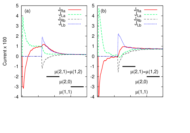
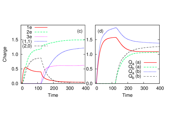
Figure 2: (Color online) (a)-(b): The total currents in the leads for two bias windows: (a) $\mu_{\rm La}=\mu_{\rm Lb}=4.25$, $\mu_{\rm Ra}=\mu_{\rm Rb}=3.75$; (b) $\mu_{\rm La}=\mu_{\rm Lb}=4.75$, $\mu_{\rm Ra}=\mu_{\rm Rb}=4.35$. The insets show the bias windows and the MES chemical potentials. (c) Partial charge for the states involved in (a) (see text); (d) Total charge on each dot for (a) and (b).

To explain what is going on we show in Fig. 2(c) the population of the relevant states for the first case, calculated with Eq. (4). As long as $\mathrm{QD_{b}}$ is closed one- and two-particle states of $\mathrm{QD_{a}}$ are charging yielding a total charge up to $Q_{a}\approx 1.5$, as further shown in Fig. 2(d). Once $\mathrm{QD_{b}}$ opens the electrons tunneling into it repel some charge from $\mathrm{QD_{a}}$ and new MESs are being created like (1,1) and (2,1). Since ${\cal E}_{g}(2,0)>{\cal E}_{g}(1,1)$ the new two-particle ground state is (1,1) and hence the transition $(2,0)\to(1,1)$ occurs, but also $(2,0)\to(2,1)$. The later is possible because ${\cal E}_{g}(2,1)-{\cal E}_{g}(2,0)=3.72$ is slightly below the bias window. Consequently the states (2,0) depopulate fast whereas the populations of the states (1,1) and $(2,1)$ (and $(1,2)$ as well) increase, as seen in Fig. 2(c). In the steady state the bias window is nearly empty of any MES chemical potential and consequently the currents nearly vanish. This is an interdot Coulomb blocking effect McClure . The total charge in the dots converges to 2.2 electrons. Of that 1.5 reside on two-electron states: 1.2 on the ground state (1,1), i.e.  below the bias window, and 0.3 on excited states (1,1) and MESs (2,0). Also, about 0.6 electrons are on three-particle states (2,1), i.e.  above the bias window.

In Fig. 3(a) we show the partial currents in the leads connected to $\mathrm{QD_{a}}$ carried by the two- and three-particle states. The former drop fast after $t_{b}$ during the depletion of the MES (2,0). Because $\mu(2,0)$ is almost in the center of the bias window $J_{\rm Ra,2}$ and $J_{\rm La,2}$ are very similar. The three-particle currents in $\mathrm{QD_{a}}$ are more interesting. They correspond to the states (2,1) and, surprisingly, $J_{\rm La,3}<0$ and $J_{Ra,3}>0$, meaning that $\mathrm{QD_{a}}$ ejects charge in both leads ${\rm L}_{a}$ and ${\rm R}_{a}$. The resulting “lobe” shape is also seen in Fig. 2(a). The net charging of the (2,1) states is actually done through the leads connected to $\mathrm{QD_{b}}$, as can be seen in Fig. 3(b), where $J_{\rm Lb,3}>0$ and $J_{\rm Rb,3}<0$, i.e. both currents flow into the dot.

Figure 3: (Color online) The partial currents carried by the two- and three-particle states in $\mathrm{QD_{a}}$ and $\mathrm{QD_{b}}$: (a-b) corresponding to Fig. 2(a); (c-d) corresponding to Fig. 2(b).

We return now to the positive correlation case. For $t<t_{b}$ no chemical potential of type $\mu(N_{a},0)$ is inside the bias window and hence no current flows in the steady state of $\mathrm{QD_{a}}$. The charging goes up to $Q_{a}\approx 1.9$ as seen in Fig. 2(d), with the ground state (2,0) occupied. When $\mathrm{QD_{b}}$ is open the new states (2,1) are created and since the corresponding $\mu(2,1)$ is inside the bias window they are available for transport. After the transient phase, when $\mathrm{QD_{b}}$ is charging and $\mathrm{QD_{a}}$ is discharging, all currents reach the same steady value, driven by the states (2,1) and (1,2) which end up equally populated. The currents in the steady state have now two- and three-particle components. These partial currents, shown in Fig. 3(c), have another curious behavior. Both $J_{\rm La,3}$ and $J_{\rm Ra,3}$ are positive in the steady state, whereas $J_{\rm La,2}$ and $J_{\rm Ra,2}$ are negative, the net result being the total, positive current. This means that three-particle currents flow from left to right, but the two-particle currents go from right to left. The reason is that in our model the electrons are created or annihilated one at a time. A MES (2,1) is formed by creating one more electron to the ground MES (1,1), and so the positive (2,1) and (1,2) currents deplete the (1,1) states. But $\mu(1,1)$ is below the bias window and so the (1,1) states have to be backfed by a negative, two-particle current. The single particle states are not occupied and do not contribute to transport. The current in the circuit $a$ is carried by MES (2,1), but not by (1,2), and the other way round in the circuit $b$. The electrons tunneling from the left leads $a$ and $b$ thus compete each other to access the (1,1) MES. In turn, when electrons leave a dot the remaining two-particle MES has the lowest energy ${\cal E}_{g}(1,1)$ and not ${\cal E}_{g}(2,0)$ which is higher. Such transitions are called “U-sensitive processes” in Ref. McClure, .

The partial currents of states (2,1) and (1,2) are shown in Fig. 4(a,b). In this case we use the same chemical potentials as in Fig. 2(b), but now $\mathrm{QD_{b}}$ contains one electron in the ground state at $t=0$. After $t=t_{b}$ $\mathrm{QD_{b}}$ absorbs more charge and the double system evolves toward the same steady state as before, Fig. 4(c). But prior to $t_{b}$, although isolated, the initial electron is being excited by the charging of $\mathrm{QD_{a}}$. This can be seen in the Fig. 4(d) where the populations of the ground state (2,1) and of the MESs containing the excited state of the electron in $\mathrm{QD_{b}}$ denoted as $(2,1_{x})$ are displayed. The currents in the circuit $a$ feel the initial electron in $\mathrm{QD_{b}}$, but also the excited states of it. Indeed the MESs $(2,1_{x})$ decay while the system approaches the steady state.

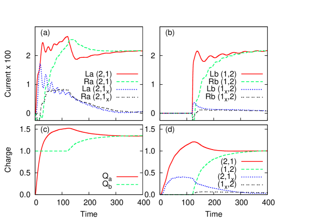
Figure 4: (Color online) (a-b) The contributions of the ground state (2,1) and of the excited states $(2,1_{x})$ to the currents in the leads. $\mu_{\rm La}=\mu_{\rm Lb}=4.75$, $\mu_{\rm Ra}=\mu_{\rm Rb}=4.35$. $\mathrm{QD_{b}}$ initially contains one electron. (c) The evolution of total charge in each dot. (d) Populations of the three-particle states.

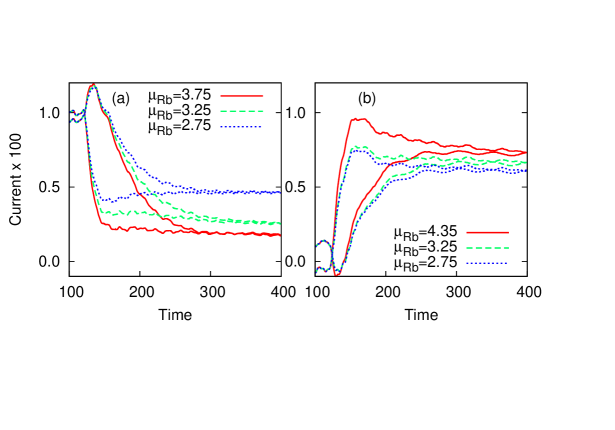
Figure 5: (Color online) The effect of the bias applied on $\mathrm{QD_{b}}$ on the currents $J_{\rm La,Ra}$. (a) $\mu_{\rm La}=\mu_{\rm Lb}=4.25,\mu_{\rm Ra}=3.75$. (b) $\mu_{\rm La}=\mu_{\rm Lb}=4.75,\mu_{\rm Ra}=4.35$. The same line type is used for the left and right currents.

Next we keep $\mu_{\rm Lb}$ fixed and decrease $\mu_{\rm Rb}$ relatively to the setup of Fig. 2(a), for increasing the bias $eV_{b}=\mu_{\rm Lb}-\mu_{\rm Rb}$. Fig. 5(a) shows that the splitting of the two currents in $\mathrm{QD_{a}}$ during the second transient phase decreases. The final current increases with $V_{b}$, but it is still smaller than the steady value before $t_{b}$. The effect of increasing $V_{b}$ on the final currents occurs in two steps. First the states (2,0) and (0,2) become slightly populated and tunneling of one electron creates three-particle currents, Fig. 5(a) with $\mu_{\rm Rb}=3,25$. Then, the bias window approaches $\mu(1,1)$ and eventually includes it, and tunneling on MES (1,1) amplifies the three-particle currents. Since $V_{b}$ is acting directly on $\mathrm{QD_{b}}$ the final currents in the $b$ circuit are larger than in $a$ (not shown). Fig. 5(b) shows the result of increasing $V_{b}$ starting with the setup of Fig. 2(b). The Coulomb blockade on $\mathrm{QD_{a}}$ is still lifted when the bias on $\mathrm{QD_{b}}$ increases. The discharging in the $a$ arm may be large enough to produce a negative left current.

Finally, one comment on the interdot distance. The interdot Coulomb interaction decreases with the distance between the dots, but for simplicity we kept it equal to the lattice constant. Increasing it the MESs change, but similar effects were obtained by appropriately tuning the chemical potentials of the leads.

IV Conclusions

In conclusion, we discussed time dependent charge sensing effects and computed mutually sensitive currents in parallel quantum dots. A steady-state transport regime of one dot is suppressed after connecting the second one. Conversely, the current through one dot increases if the charging of the second dot opens new many-body channels within the bias window. In particular, we predict that the transient current in the leads attached to the first dot may change sign when the second dot is connected. This effect can be experimentally tested.

The RDO of the coupled system and the GME describe its entangled dynamics by treating all electrons equally. The Coulomb effects are fully included and the charging and discharging energies are present in the MES structure. The classical charging and the quantum correlations are treated together. The exact many-body states fit naturally with the Fock space formulation of the GME. The access to individual MES allows a better understanding of the Coulomb-induced effects on the total currents.

- (1) M. Field, C. G. Smith, M. Pepper, D. A. Ritchie, J. E. F. Frost, G. A. C. Jones, D. G. Hasko, Phys. Rev. Lett. 70, 1311 (1993).
- (2) A. C. Johnson, C. M. Marcus, M. P. Hanson, A. C. Gossard, Phys. Rev. Lett. 93, 106803 (2004).
- (3) S. Gustavsson, R. Leturcq, B. Simovic, R. Schleser, T. Ihn, P. Studerus, K. Ensslin, D. C. Driscoll, A. C. Gossard, Phys. Rev. Lett. 96, 076605 (2006).
- (4) E. Onac, F. Balestro, L. H . Willems van Beveren, U. Hartmann, Y. V. Nazarov, L. P. Kouwenhoven, Phys. Rev. Lett. 96, 176601 (2006).
- (5) E. V. Sukhorukov, A. N. Jordan, S. Gustavsson, R. Leturcq, T. Ihn, K. Ensslin, Nature Physics 3, 243 (2007).
- (6) V. S. Khrapai, S. Ludwig, J. P. Kotthaus, H. P. Tranitz, W. Wegscheider, Phys. Rev. Lett. 97, 176803 (2006).
- (7) S. Gustavsson, M. Studer, R. Leturcq, T. Ihn, K. Ensslin, Phys. Rev. Lett. 99, 206804 (2007).
- (8) S-H. Ouyang, C-H. Lam, J.Q. You, Phys. Rev. B 81, 075301 (1010).
- (9) U. Gasser, S. Gustavsson, B. Küng, K. Ensslin, T. Ihn, D. C. Driscoll, A. C. Gossard, Phys. Rev. B 79, 035503 (2009).
- (10) D. T. McClure, L. DiCarlo, Y. Zhang, H.-A. Engel, C. M. Marcus, M. P. Hanson, A. C. Gossard, Phys. Rev. Lett. 98, 056801 (2007).
- (11) M. Büttiker, Phys. Rev. Lett. 65, 2901 (1990); Phys. Rev. B 46, 12485 (1992).
- (12) M. C. Goorden and M. Büttiker, Phys. Rev. Lett. 99, 146801 (2007).
- (13) V. Moldoveanu and B. Tanatar, Europhys. Lett. 86, 67004 (2009).
- (14) A. Levchenko and A. Kamenev, Phys. Rev. Lett. 101, 216806 (2008).
- (15) R. Sanchez, R. Lapez, D. Sanchez, M. Büttiker, Phys. Rev. Lett. 104, 076801 (2010).
- (16) S. Welack, M. Esposito, U. Harbola, S. Mukamel, Phys. Rev. B 77, 195315 (2008).
- (17) T. M. Stace and S. D. Barrett, Phys. Rev. Lett. 92, 136802 (2004).
- (18) For example: J. Rammer, A. L. Shelankov, and J. Wabnig, Phys. Rev. B 70, 115327 (2004); U. Harbola, M. Esposito, and S. Mukamel, Phys. Rev. B 74, 235309 (2006).
- (19) V. Moldoveanu, A. Manolescu, V. Gudmundsson, New. J. Phys. 11, 073019 (2009).
- (20) V. Gudmundsson, C. Gainar, C. S. Tang, V. Moldoveanu, A. Manolescu, New J. Phys. 11, 113007 (2009).
- (21) V. Moldoveanu, A. Manolescu, V. Gudmundsson, Phys. Rev. B 80, 205325 (2009).
- (22) V. Moldoveanu, A. Manolescu, C. S. Tang, V. Gudmundsson, Phys. Rev. B 81, 155442 (2010).