Mass hierarchies and non-decoupling in multi-scalar field dynamics

Abstract

In this work we study the effects of field space curvature on scalar field perturbations around an arbitrary background field trajectory evolving in time. Non-trivial imprints of the ‘heavy’ directions on the low energy dynamics arise when the vacuum manifold of the potential does not coincide with the span of geodesics defined by the sigma model metric of the full theory. When the kinetic energy is small compared to the potential energy, the field traverses a curve close to the vacuum manifold of the potential. The curvature of the path followed by the fields can still have a profound influence on the perturbations as modes parallel to the trajectory mix with those normal to it if the trajectory turns sharply enough. We analyze the dynamical mixing between these non-decoupled degrees of freedom and deduce its non-trivial contribution to the low energy effective theory for the light modes. We also discuss the consequences of this mixing for various scenarios where multiple scalar fields play a vital role, such as inflation and low-energy compactifications of string theory.

I Introduction and summary

A thorough and tractable understanding of early universe physics through an ultraviolet (UV) complete description, such as string theory, remains out of our reach for now. While we do not completely understand the precise features of the UV completion of the standard model coupled to gravity, or even the gross structure of such a putative theory, one of its likely generic consequences is the presence of a large number of scalar fields and possibly a large number of vacua. The masses of these fields are typically associated with the internal structure of the theory, for example, the cutoff scale of the effective action which encapsulates the UV relevant physics that completes our theory.

However, in general it might be that different fields have different mass scales associated with them such that a hierarchy appears in the field content, and we can colloquially speak of ‘light’ and ‘heavy’ modes. Usually, the heavy fields are assumed to be integrated out since they are kinematically inaccessible provided that their masses are larger than the scale of physics of interest. However in reality, we cannot completely ignore the heavy fields as the conditions underlying the decoupling theorem of Ref. Appelquist:1974tg can sometimes be relaxed, for instance through time dependence in the heavy sector, or through dynamical mixing of heavy and light sectors. In the context of field theories at a point in field space, gauge symmetry breaking can lead to a non-decoupling scenario (see SekharChivukula:2007gi , and references therein, for a recent example). In the context of supergravity, decoupling of heavy fields is still actively being studied Choi:2004sx ; deAlwis:2005tg ; deAlwis:2005tf ; Binetruy:2004hh ; Achucarro:2007qa ; Achucarro:2008sy ; Achucarro:2008fk ; BenDayan:2008dv ; Gallego:2008qi ; Brizi:2009nn ; Gallego:2009px ; Gallego:2011jm .

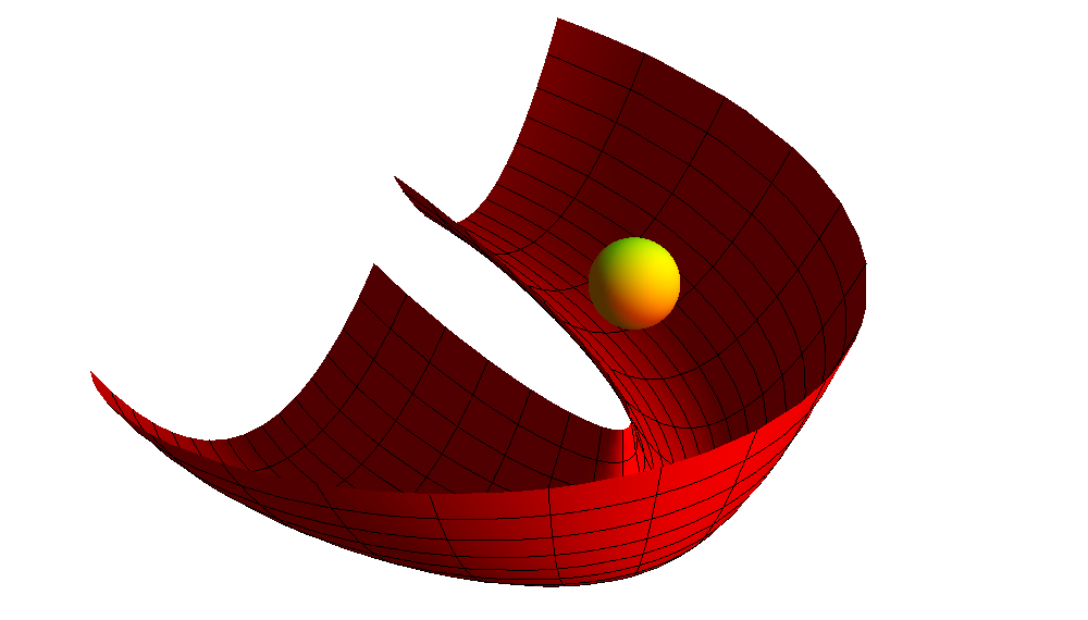
Figure 1: A curved trajectory with a sudden bend, where a scalar potential presents a turning flat direction with a massive mode remaining perpendicular to it

In a series of papers, this collaboration will examine the conditions under which decoupling is relaxed, or fails outright, and explore quantitatively the consequences of this failure. The subject of this paper is to study multi-scalar field theories in Minkowski spacetimes characterized by having a hierarchy of scales between different families of fields. Our main goal is to characterize the interaction between light and heavy degrees of freedom as the background expectation value of the scalar fields (which we assume to be spatially homogeneous) varies in time, traversing a curved trajectory in field space. Specifically, we analyze those situations where the heavy degrees of freedom correspond to the transverse modes with respect to the path followed by the background fields. Pictorially, these curved trajectories are placed in the nearly flat valleys of the vacuum manifold. An example of such a curved trajectory is schematically shown in Fig. 1 where a scalar potential presents a curved flat direction with a massive mode remaining perpendicular to it. Such curvature mixes light and heavy directions along the field trajectory, possibly non-adiabatically if the field space is ‘curved’ enough. In the context of inflation, the effects studied in this work lead to potentially observable effects in the spectrum of primordial perturbations (see Achucarro:2010da and references therein).

In the case of two-field models, we will show that whenever the trajectory makes a turn in field space such that the light direction is interchanged by a heavy direction (and vice versa), the low energy effective action describing the dynamics of the light degrees of freedom generically picks up a non-trivial correction, hereby parameterized by $\beta$ and given by

$$\beta=\ln\left(1+\frac{4\dot{\phi}_{0}^{2}}{\kappa^{2}M_{H}^{2}}\right)\,,$$ (1.1)

where $\dot{\phi}_{0}$ is the velocity of the background scalar field, $\kappa$ is the radius of curvature characterizing the bending of the trajectory in field space, and $M_{H}$ is the characteristic mass scale of the heavy modes. We emphasize that the bending is measured with respect to the geodesics of the sigma model metric, whether or not it is canonical; notice that $\kappa$ represents a distance measured in the geometrical space of scalar fields, and therefore it has units of mass.

More precisely, at low energies ($k\ll M_{H}$) the equation of motion describing the scalar field fluctuation parallel to the trajectory of background fields is found to be

$$\ddot{\varphi}-e^{-\beta}\nabla^{2}\varphi+M^{2}_{L}\,\varphi=0\,,$$ (1.2)

with $\nabla^{2}\equiv\delta^{ij}\partial_{i}\partial_{j}$ being the spatial Laplacian: see (4.55). Thus the kinetic energy term is modified by a factor of $e^{-\beta}$ in front of the spatial gradient term, in agreement with Tolley:2009fg . In the context of inflation, this can give rise to sizable effects that may be observable in the next generation of the cosmic microwave background observations. For example, for inflation in supergravity models, the masses of heavy degrees of freedom during inflation are typically of order $M_{H}=\mathcal{O}(H)$, with $H$ being the Hubble parameter during inflation. This leads to the naive expectation

$$e^{\beta}\sim 1+\epsilon\frac{M_{\rm Pl}^{2}}{\kappa^{2}}\,,$$ (1.3)

where $\epsilon\equiv-\dot{H}/H^{2}=(\dot{\phi}_{0}/H)^{2}/(2M_{\rm Pl}^{2})$ is the so-called slow-roll parameter. Then, if the bending of the trajectory is such that the radius of curvature $\kappa$ becomes much smaller than $M_{\rm Pl}$ one then is led to $e^{\beta}\gg 1$. Such a situation implies strong modifications on the scale dependence of inflaton fluctuations, contributing non-trivial features to the power spectrum well within the threshold of detection. The full analysis valid for inflationary cosmology is, however, more involved than the naive arguments above as it requires a detailed account of gravity and careful treatments of the multi-field dynamics at horizon crossing. For this reason, in the present note we study the basic features of the effects of the heavy-light field interactions during turns of the scalar field trajectory in a Minkowski background, and leave the study of inflationary de Sitter case for a separate paper Achucarro:2010da . We stress here that the perspective that follows from our analysis is that the only relevant criteria for the effects we uncover (such as the modified speed of sound for the perturbations) is that our system deviates sufficiently from a geodesic trajectory .

Our formalism, and its application to inflation Achucarro:2010da builds upon previous work GrootNibbelink:2000vx ; GrootNibbelink:2001qt ; Gordon:2000hv ; Nilles:2001fg that we extend to be able to account for the effects coming from very sharp turns and also prolonged turns in which the true ground state deviates significantly from its single-field approximation. By disregarding the effects of gravity, we are able to describe in detail the evolution of the quantum modes in some idealized settings (e.g. turns at a constant rate). We also extend recent results by Chen:2009we ; Tolley:2009fg , that we recover in the right limits. In particular, we are able to clarify the relevance or otherwise of non-canonical kinetic terms, in particular with respect to a reduced speed of sound in the effective low energy theory (see also sera ). We expect our results to be relevant for any phenomena where the variation of vacuum expectation values plays a significant role, such us inflation, phase transitions, soliton interactions and soliton-radiation scattering.

In the remainder of this paper, we will first elaborate on the general framework and study the background equations of motion in Section II. In Section III, we will study the theory of perturbations and the quantization around a general field trajectory. In Section IV, we will apply the theory to the case of a large hierarchy between light and heavy degrees of freedom that span a curved field space trajectory. To conclude, we will discuss some applications in Section V, in particular regarding inflation and the decoupling of heavy modes in supergravity. Some calculational details are provided in the appendices.

II Geometry of multi-scalar field models

We are interested in multi-scalar field theories admitting a low energy effective action consisting of at most two space-time derivatives. Examples of such theories are low energy compactifications of string theory and supergravity models, where the number of scalar degrees of freedom (often referred to as moduli) can be considerably large. For an arbitrary number $n_{\rm tot}$ of scalar fields in a Minkowski background, the effective action of such a theory may be written in the form

$$S=-\int d^{4}x\left[\frac{1}{2}\gamma_{ab}\partial^{\mu}\phi^{a}\partial_{\mu}\phi^{b}+V(\phi)\right]\,,$$ (2.1)

where $\phi^{a}$, with $a=1,\cdots n_{\rm tot}$, is a set of scalar fields and $\gamma_{ab}=\gamma_{ab}(\phi)$ is an arbitrary symmetric matrix restricted to be positive definite. Any contribution to this action containing higher space-time derivatives will be suppressed by some cutoff energy scale $\Lambda$, which we assume to be much larger than the energy scale of our interest. In low energy string compactifications, such a scale $\Lambda$ corresponds to the compactification scale, which may be close to $M_{\rm Pl}$. However, as mentioned before, we do not consider coupling this theory to gravity, saving this for a separate report Achucarro:2010da .

In order to study the dynamics of the present system it is useful to think of $\gamma_{ab}$ as a metric tensor of some abstract scalar manifold $\mathcal{M}$ of dimension $n_{\rm tot}$. This allows us to consider the definition of several standard geometrical quantities related to $\mathcal{M}$. For instance, the Christoffel connections are given by

$$\Gamma^{a}_{bc}=\frac{1}{2}\gamma^{ad}\left(\partial_{b}\gamma_{dc}+\partial_{c}\gamma_{bd}-\partial_{d}\gamma_{bc}\right)\,,$$ (2.2)

where $\gamma^{ab}$ is the inverse metric satisfying $\gamma^{ac}\gamma_{cb}=\delta^{a}{}_{b}$, and $\partial_{a}$ denotes a partial derivative with respect to $\phi^{a}$. This allows us to define covariant derivatives in the usual way as $\nabla_{a}X_{b}\equiv\partial_{a}X_{b}-\Gamma_{ab}^{c}X_{c}$. Also, we may define the associated Riemann tensor as

$$\mathcal{R}^{a}{}_{bcd}\equiv\partial_{c}\Gamma^{a}_{bd}-\partial_{d}\Gamma^{a}_{bc}+\Gamma^{a}_{ce}\Gamma^{e}_{db}-\Gamma^{a}_{de}\Gamma^{e}_{cb}\,.$$ (2.3)

as well as the Ricci tensor $\mathcal{R}_{ab}=\mathcal{R}^{c}{}_{acb}$ and the Ricci scalar $\mathcal{R}=\gamma^{ab}\mathcal{R}_{ab}$. We should keep in mind that, typically, there will be an energy scale $\Lambda_{\mathcal{M}}$ associated with the curvature of $\mathcal{M}$, fixing the typical mass scale of the Ricci scalar as $\mathcal{R}\sim\Lambda_{\mathcal{M}}^{-2}$. In many concrete situations the scale $\Lambda_{\mathcal{M}}$ corresponds precisely to the aforementioned cutoff scale $\Lambda$. For example, in $N=1$ supergravity realizations of string compactifications, one typically finds that the Ricci scalar of the Kähler manifold satisfies $\mathcal{R}\sim M_{\rm Pl}^{-2}$ GomezReino:2006wv ; Covi:2008ea . In the following, we assume $\Lambda\sim\Lambda_{\mathcal{M}}$ and do not distinguish them.

Given these geometric quantities, we can write the background equation of motion of the homogeneous background fields $\phi_{0}^{a}=\phi_{0}^{a}(t)$ from the action (2.1). If $\dot{\phi}_{0a}\dot{\phi}_{0}^{a}\neq 0$, one may think of $\phi_{0}^{a}(t)$ as the coordinates parametrizing a trajectory in $\mathcal{M}$, where $t$ is the parameter on the curve describing the expectation value of the scalar fields. Before proceeding with a detailed analysis of these trajectories, let us emphazise that these trajectories may or may not be the geodesics of $\mathcal{M}$, with the details depending on the specific form of the scalar potential $V(\phi)$ and the geometry of $\mathcal{M}$. Varying the action (2.1) with respect to $\phi^{a}$, the equations of motion of $\phi^{a}$ are then found to be

$$\frac{D}{dt}\dot{\phi}_{0}^{a}+V^{a}=0\,,$$ (2.4)

where we have introduced the notation $DX^{a}\equiv dX^{a}+\Gamma^{a}_{bc}X^{b}d\phi_{0}^{c}$ and $V^{a}\equiv\gamma^{ab}\partial_{b}V$. Given a certain scalar manifold $\mathcal{M}$ and a scalar potential $V$, these equations can be solved to obtain the trajectory in $\mathcal{M}$ traversed by the background scalar fields. It is convenient to define the rate of variation of the scalar fields $\dot{\phi}_{0}$ along the trajectory as

$$\dot{\phi}_{0}^{2}\equiv\gamma_{ab}\dot{\phi}_{0}^{a}\dot{\phi}_{0}^{b}\,.$$ (2.5)

Since $\gamma_{ab}$ is positive definite, $\dot{\phi}_{0}^{2}$ is always greater than or equal to zero. Without loss of generality, in what follows we assume that $\dot{\phi}(t)>0$ for all $t$. Then the unit tangent vector $T^{a}$ to the trajectory is defined as

$$T^{a}\equiv\frac{\dot{\phi}_{0}^{a}}{\dot{\phi}_{0}}\,,$$ (2.6)

and if the trajectory is curved we can define one of the normal vectors to be

$$N^{a}\equiv s_{N}(t)\left(\gamma_{bc}\frac{DT^{b}}{dt}\frac{DT^{c}}{dt}\right)^{-1/2}\frac{DT^{a}}{dt}\,,$$ (2.7)

where $s_{N}(t)=\pm 1$ denotes the orientation of $N^{a}$ with respect to the vector $DT^{a}/dt$. That is, if $s_{N}(t)=+1$ then $N^{a}$ is pointing in the same direction as $DT^{a}/dt$, whereas if $s_{N}(t)=-1$ then $N^{a}$ is pointing in the opposite direction. Due to the presence of the square root, it is clear that $N^{a}$ is only well defined at intervals where $DT^{a}/dt\neq 0$. However, since $DT^{a}/dt$ may become zero at finite values of $t$, we allow $s_{N}(t)$ to flip signs each time this happens in such a way that both $N^{a}$ and $DT^{a}/dt$ remain a continuous function of $t$. This implies that the sign of $s_{N}$ may be chosen conventionally at some initial time $t_{i}$, but from then on it is subject to the equations of motion respected by the background . As we shall see later, in the particular case where $\mathcal{M}$ is two dimensional, the presence of $s_{N}(t)$ in (2.7) is sufficient for $N^{a}$ to have a fixed orientation with respect to $T^{a}$ (either left-handed or right-handed).

After some formal manipulations, we can deduce $\kappa$, the radius of curvature of the trajectory followed by the vacuum expectation value $\phi_{0}^{a}(t)$, as

$$\frac{1}{\kappa}=\frac{|V_{N}|}{\dot{\phi}_{0}^{2}}\,,$$ (2.8)

where $V_{N}\equiv N^{a}V_{a}$. Details of how (2.8) is derived can be found in Appendix A. Notice that for $\dot{\phi}_{0}\neq 0$, the only way of having $V_{N}=0$ is by following a straight curve for which there is no geodesic deviation, $DT^{a}/dt=0$. This result follows the basic intuition that, during a turn in the trajectory, the scalar fields will shift from the minimum of the potential $V_{N}=0$ along the perpendicular direction $N^{a}$. Trajectories for which $V_{N}=0$ are in fact geodesics, and therefore the parameter $\kappa$ is a useful measure of the geodesic deviation caused by the potential $V$. On dimensional grounds, we should expect $\kappa^{-1}\sim\Lambda_{M}^{-1}$, as the intrinsic curvature of the manifold $M$ is the result of the embedding in a yet higher energy completion, and this likely bestows this manifold with a similar extrinsic curvature scale. This extrinsic curvature is then necessarily the minimal extrinsic curvature for any trajectory on $M$. Yet, much more curved trajectories are perfectly possible  and we therefore allow a wider range of values for $\kappa$.

III Perturbation theory and its quantization

We now study the evolution of the scalar field fluctuations around the background time-dependent solution examined in the previous section. We extend the formalism of GrootNibbelink:2000vx ; Nilles:2001fg ; GrootNibbelink:2001qt to be able to deal with regimes of fast and or continuous turns. As we shall see, the radius of curvature $\kappa$ couples the perturbations parallel and normal to the motion of the background fields. Let us start by writing $\phi^{a}$ including perturbations $\delta\phi^{a}(t,{\bf x})\equiv\varphi^{a}(t,{\bf x})$ as

$$\phi^{a}(t,{\bf x})=\phi_{0}^{a}(t)+\varphi^{a}(t,{\bf x})\,,$$ (3.1)

where $\phi_{0}^{a}(t)$ corresponds to the exact solution to the homogeneous equation of motion (2.4). Starting from the action (2.1), one finds the equations of motion for $\varphi^{a}$ as

$$\frac{D^{2}\varphi^{a}}{dt^{2}}-\nabla^{2}\varphi^{a}+C^{a}_{\phantom{a}b}\varphi^{b}=0\,,$$ (3.2)

where

$$C^{a}_{\phantom{a}b}=\nabla_{b}V^{a}-\dot{\phi}_{0}^{2}\,\mathcal{R}^{a}_{\phantom{a}cdb}T^{c}T^{d}\,.$$ (3.3)

It is convenient to rewrite these equations in terms of a new set of perturbations orthogonal to each other. For this we define a complete set of vielbeins $e^{I}_{a}$ and work with redefined fields

$$v^{I}=e^{I}_{a}\varphi^{a}\,.$$ (3.4)

An example of a possible choice for these vielbeins is a set $\left\{e^{I}_{a}\right\}$ with $T_{a}$ and $N_{a}$ among its elements Gordon:2000hv , but we do not consider this choice until later. Recall that the vielbeins satisfy the basic relations $\delta_{IJ}e^{I}_{a}e^{J}_{b}=\gamma_{ab}$ and $\gamma^{ab}e^{I}_{a}e^{J}_{b}=\delta^{IJ}$, which lead to

$$e^{I}_{a}\frac{D}{dt}e^{a}_{J} = -e^{a}_{J}\frac{D}{dt}e^{I}_{a}\,,$$ (3.5)

$$e^{a}_{I}\frac{D}{dt}e_{b}^{I} = -e_{b}^{I}\frac{D}{dt}e_{I}^{a}\,.$$ (3.6)

In (3.4) the $\varphi^{a}$ are vectors with respect to the covariant derivative $D/dt$, while the fields $v^{I}$ are scalars. Then, it is easy to show that

$$\dot{v}^{I} = e^{I}_{a}\frac{D\varphi^{a}}{dt}-Z^{I}_{\,\,\,J}v^{J}\,,$$ (3.7)

$$\ddot{v}^{I} = e^{I}_{a}\frac{D^{2}\varphi^{a}}{dt^{2}}-2Z^{I}_{\,\,\,J}\dot{v}^{J}-\left(Z^{I}_{\,\,\,K}Z^{K}_{\phantom{a}J}+\dot{Z}^{I}_{\,\,\,J}\right)v^{J},\quad$$ (3.8)

where we have introduced the antisymmetric matrix $Z^{I}_{\,\,\,J}$ as

$$Z^{I}_{\,\,\,J}=e^{I}_{a}\frac{D}{dt}e^{a}_{J}\,.$$ (3.9)

Notice that $Z^{I}_{\,\,\,J}=\left(e^{I}_{a}\partial_{b}e^{a}_{J}+e^{I}_{a}\Gamma^{a}_{bc}e^{c}_{J}\right)\dot{\phi}_{0}^{b}=\omega_{b\,\,\,J}^{\,\,\,I}\dot{\phi}_{0}^{b},$ where $\omega_{b\,\,\,J}^{\,\,\,I}$ are the usual spin connections for non-coordinate basis, therefore $Z^{I}_{\,\,\,J}$ can be used to define a covariant derivative acting on the $v^{I}$-fields as

$$\frac{\mathcal{D}}{dt}v^{I}\equiv\dot{v}^{I}+Z^{I}_{\,\,\,J}v^{J}\,.$$ (3.10)

From (3.7) and (3.8), we can see that this new covariant derivative is related to the original covariant derivative as

$$\frac{\mathcal{D}}{dt}v^{I} = e^{I}_{a}\frac{D}{dt}\varphi^{a}\,,$$ (3.11)

$$\frac{{\mathcal{D}}^{2}}{dt^{2}}v^{I} = e^{I}_{a}\frac{D^{2}}{dt^{2}}\varphi^{a}\,.$$ (3.12)

One can verify that this derivative is compatible with the Kronecker delta in the sense that $\mathcal{D}\delta_{IJ}/dt=0$. Then, it is easy to show that the equation of motion (3.2) in terms of the new perturbations $v^{I}$ becomes

$$\frac{{\mathcal{D}}^{2}}{dt^{2}}v^{I}-\nabla^{2}v^{I}+C^{I}_{\,\,J}v^{J}=0\,,$$ (3.13)

where $C^{I}{}_{J}\equiv e^{I}_{a}e^{b}_{J}C^{a}_{\phantom{a}b}$.

III.1 Canonical frame

In introducing the vielbeins in the previous section, we have not specified any alignment of the moving frame. In fact, given an arbitrary frame $e^{I}_{a}$, it is always possible to find a ‘canonical’ frame where the scalar field perturbations acquire canonical kinetic terms in the action. To find it, let us introduce a new set of fields $u^{I}$ defined from the original ones $v^{I}$ in the following way:

$$v^{I}(t)=R^{I}_{\phantom{I}J}(t,t_{0})u^{J}(t)\,.$$ (3.14)

Here, $R^{I}_{\phantom{I}J}(t,t_{0})$ is a matrix satisfying the first order differential equation

$$\frac{d}{dt}R^{I}_{\phantom{I}J}=-Z^{I}_{\phantom{I}K}R^{K}_{\phantom{K}J}\,,$$ (3.15)

with the boundary condition $R^{I}_{\phantom{I}J}(t_{0},t_{0})=\delta^{I}{}_{J}$. By defining a new matrix $S^{I}_{\phantom{I}J}$ to be the inverse of $R^{I}_{\phantom{I}J}$, namely $S^{I}_{\phantom{I}K}R^{K}_{\phantom{K}J}=R^{I}_{\phantom{I}K}S^{K}_{\phantom{K}J}=\delta^{I}{}_{J}$, it is not difficult to see that $S^{I}_{\phantom{I}J}$ satisfies

$$\frac{d}{dt}S_{I}^{\phantom{I}J}=-Z^{J}_{\phantom{J}K}S_{I}^{\phantom{I}K}\,,$$ (3.16)

where we used the fact that $Z$ is antisymmetric in its indices $Z_{IJ}=-Z_{JI}$. Since both solutions to (3.15) and (3.16) are unique, the previous equation tells us that $S_{IJ}=R_{JI}$. Thus, $S$ corresponds to $R^{T}$, the transpose of $R$. This means that for a fixed time $t$, $R_{IJ}(t,t_{0})$ is an element of the orthogonal group O$(n_{\rm tot})$, the group of matrices $R$ satisfying $RR^{T}=1$. The solution of (3.15) is well known, and may be symbolically written as

$$R(t,t_{0}) = 1+\sum_{n=1}^{\infty}\frac{(-1)^{n}}{n!}\!\!\int_{t_{0}}^{t}\mathbb{T}\left[Z(t_{1})\cdots Z(t_{n})\right]d^{n}t$$ (3.17)

$$= \mathbb{T}\exp\left[-\int_{t_{0}}^{t}\!\!\!dt\,Z(t)\right]\,,$$

where $\mathbb{T}$ stands for the time ordering symbol. That is: $\mathbb{T}[Z(t_{1})Z(t_{2})\cdots Z(t_{n})]$ corresponds to the product of $n$ matrices $Z(t_{i})$ for which $t_{1}\geq t_{2}\geq\cdots\geq t_{n}$. Coming back to the $u^{I}$-fields, it is possible to see now that, by virtue of (3.15) one has

$$\frac{\mathcal{D}v^{I}}{dt} = R^{I}_{\phantom{I}J}\frac{du^{J}}{dt}\,,$$ (3.18)

$$\frac{\mathcal{D}^{2}v^{I}}{dt^{2}} = R^{I}_{\phantom{I}J}\frac{d^{2}u^{J}}{dt^{2}}\,.$$ (3.19)

Inserting these relations back into the equation of motion (3.13), we obtain the equation of motion for the $u^{I}$-fields as

$$\frac{d^{2}u^{I}}{dt^{2}}-\nabla^{2}u^{I}+\left[R^{T}(t)\,C\,R(t)\right]^{I}_{\phantom{I}J}u^{J}=0\,.$$ (3.20)

This equation of motion can be derived from an action

$$S = \frac{1}{2}\int d^{4}x\big{\{}\dot{u}^{I}\dot{u}_{I}-\nabla u^{I}\cdot\nabla u_{I}$$ (3.21)

$$\qquad-\left[R^{T}(t)CR(t)\right]_{IJ}u^{I}u^{J}\big{\}}\,.$$

Thus, we see that the $u^{I}$-fields correspond to the canonical fields in the usual sense. To finish, let us notice that by construction, at the initial time $t_{0}$, the canonical fields $u^{I}$ and the original fields $v^{I}$ coincide, $u^{I}(t_{0})=v^{I}(t_{0})$. Obviously, it is always possible to redefine a new set of canonical fields by performing an orthogonal transformation.

III.2 Quantization of the system

Having the canonical frame at hand, we may now quantize the system in the usual way. Starting from the action (3.21), the canonical momentum conjugate to $u^{I}$ is given by $\Pi_{u}^{I}=du^{I}/dt$. To quantize the system, we then demand this pair to satisfy the canonical commutation relations

$$\left[u^{I}({\bf x},t),\Pi_{u}^{J}({\bf y},t)\right] = i\delta^{IJ}\delta^{(3)}({\bf x}-{\bf y})\,,$$ (3.22)

with all other commutators vanishing. With the help of the $R$ transformation introduced in (3.14), we can define commutation relations which are valid in an arbitrary moving frame. More precisely, we are free to define a new canonical pair $v^{I}$ and $\Pi^{I}_{v}$ given by

$$v^{I} = R^{I}_{\phantom{I}J}u^{J}\,,$$ (3.23)

$$\Pi_{v}^{I} \equiv \frac{\mathcal{D}}{dt}v^{I}=R^{I}_{\phantom{I}J}(t,t_{0})\Pi_{u}^{J}\,.$$ (3.24)

This pair is found to satisfy similar commutation relations GrootNibbelink:2001qt

$$\left[v^{I}({\bf x},t),\Pi_{v}^{J}({\bf y},t)\right]=i\delta^{IJ}\delta^{(3)}({\bf x}-{\bf y})\,.$$ (3.25)

It is in fact possible to obtain an explicit expression for $v^{I}({\bf x},t)$ in terms of creation and annihilation operators. For this, let us write $v^{I}({\bf x},t)$ as a sum of Fourier modes

$$v^{I}({\bf x},t) = \frac{1}{(2\pi)^{3/2}}\sum_{\alpha}\int d^{3}k\big{[}e^{i{\bf k}\cdot{\bf x}}\,v_{\alpha}^{I}(k,t)\,a_{\alpha}({\bf k})$$ (3.26)

$$\qquad+e^{-i{\bf k}\cdot{\bf x}}\,v_{\alpha}^{I*}(k,t)\,a^{{\dagger}}_{\alpha}({\bf k})\big{]}\,,$$

where we have anticipated the need of expressing $v^{I}({\bf x},t)$ as a linear combination of $n_{\rm tot}$ time-independent creation and annihilation operators $a^{{\dagger}}_{\alpha}({\bf k})$ and $a_{\alpha}({\bf k})$ respectively, with $\alpha=1,\cdots,n_{\rm tot}$. These operators are required to satisfy the usual commutation relations

$$\left[a_{\alpha}({\bf k}),a_{\beta}^{{\dagger}}({\bf k^{\prime}})\right]=\delta_{\alpha\beta}\delta^{(3)}({\bf k}-{\bf k^{\prime}})\,,$$ (3.27)

otherwise zero. Since the operators $a^{{\dagger}}_{\alpha}({\bf k})$, for different $\alpha$, are taken to be linearly independent, the time-dependent coefficients $v_{\alpha}^{I}(k,t)$ in (3.26) must satisfy $n_{\rm tot}$ independent equations (one for each value of $\alpha$) given by

$$\frac{\mathcal{D}^{2}}{dt^{2}}v_{\alpha}^{I}(t,k)+k^{2}v_{\alpha}^{I}(k,t)+C^{I}_{\phantom{I}J}v_{\alpha}^{J}(k,t)=0\,,$$ (3.28)

which follows from (3.13). Of course, there must exist $n_{\rm tot}$ independent solutions $v_{\alpha}^{I}(k,t)$ to this equation. For definiteness, at a given initial time $t=t_{0}$ we are allowed to choose each mode to satisfy the following orthogonal initial conditions

$$v_{1}^{I}=\left(\begin{array}[]{c}1\\ 0\\ \vdots\\ 0\end{array}\right)v_{1}(k),\quad v_{2}^{I}=\left(\begin{array}[]{c}0\\ 1\\ \vdots\\ 0\end{array}\right)v_{2}(k),\quad\cdots\quad v_{n_{\rm tot}}^{I}=\left(\begin{array}[]{c}0\\ 0\\ \vdots\\ 1\end{array}\right)v_{n_{\rm tot}}(k),$$ (3.29)

and initial momenta

$$\frac{\mathcal{D}v_{1}^{I}}{dt}=\left(\begin{array}[]{c}1\\ 0\\ \vdots\\ 0\end{array}\right)\pi_{1}(k),\quad\frac{\mathcal{D}v_{2}^{I}}{dt}=\left(\begin{array}[]{c}0\\ 1\\ \vdots\\ 0\end{array}\right)\pi_{2}(k),\quad\cdots\quad\frac{\mathcal{D}v_{n_{\rm tot}}^{I}}{dt}=\left(\begin{array}[]{c}0\\ 0\\ \vdots\\ 1\end{array}\right)\pi_{n_{\rm tot}}(k),$$ (3.30)

where each unit vector refers to a direction in the tangent space labelled by the $I$-index, and $v_{\alpha}(k)$ and $\pi_{\alpha}(k)$ are the factors defining the amplitude of the initial conditions. Since the operator $\mathcal{D}/dt=\partial/\partial t+Z$ mixes different directions in the $v^{I}$-field space and since in general the time-dependent matrix $C_{IJ}$ is non-diagonal, then the mode solutions $v_{\alpha}^{I}(k,t)$ satisfying the initial conditions (3.29) and (3.30) will not necessarily remain pointing in the same direction nor will they remain orthogonal at an arbitrary time $t\neq t_{0}$. Therefore, each mode solution labelled by $\alpha$ will provide a linearly independent vector which is allowed to vary its direction in the field space labelled by the $I$-index, which is why one needs to distinguish between the two set of indices. In other words the $I$-index labels the system of coupled oscillators while the $\alpha$-index labels the modes.

In Appendix B we show that it is always possible to choose initial conditions for $v_{\alpha}^{I}(k,t)$ and $\mathcal{D}v_{\alpha}^{I}(k,t)/dt$ such that the commutation relations (3.25) are ensured. The choice of the initial conditions in (3.29) and (3.30) is a convenient one, as it is not difficult to verify that with this choice and the requirement on $v_{\alpha}(k)$ and $\pi_{\alpha}(k)$ such that

$$v_{\alpha}(k)\pi_{\alpha}^{*}(k)-v_{\alpha}^{*}(k)\pi_{\alpha}(k)=i,$$ (3.31)

and the commutation relations (3.25) are automatically satisfied for all times. We should emphazise however that, as discussed in the appendix, this is not the unique choice for initial conditions. In general, any choice satisfying conditions (B.14) and (B.15) deduced and discussed in Appendix B will do just fine.

IV Dynamics in the presence of mass hierarchies

The main quantity determining the dynamics of the present system is the scalar potential $V(\phi)$. Since we are interested in studying the dynamics of multi-scalar field theories in Minkowski space-time, we will assume that it is positive definite, $V(\phi)\geq 0$. From the potential one can define the mass matrix $M^{2}_{ab}$ associated to the scalar fluctuations around a given vacuum expectation value $\langle\phi^{a}\rangle=\phi^{a}_{0}$ as

$$M^{2}_{ab}(\phi_{0})\equiv\nabla_{a}\nabla_{b}V\big{|}_{\phi=\phi_{0}}\,.$$ (4.1)

In general this definition renders a non-diagonal mass matrix, yet it is always possible to find a ‘local’ frame in which it becomes diagonal, where the entries are given by the eigenvalues $m_{a}^{2}$. Now, we take into account the existence of hierarchies among different families of scalar fields, and specifically consider two families, herein referred to as heavy and light fields which are characterized by

$$m^{2}_{H}\gg m^{2}_{L}\,.$$ (4.2)

In the particular case where the vacuum expectation value of the scalar fields remains constant $\dot{\phi}^{a}_{0}=0$, it is well understood that the heavy fields can be systematically integrated out, providing corrections of $\mathcal{O}(k^{2}/m^{2}_{H})$ with $k$ being the energy scale of interest to the low energy effective Lagrangian describing the remaining light degrees of freedom Appelquist:1974tg . If however the vacuum expectation value $\phi^{a}_{0}$ is allowed to vary with time, new effects start occurring which can be significant at low energies. Naively speaking, given the mass matrix (4.1) one would say that a hierarchy between the directions $T^{a}$ and $N^{a}$ is present if

$$T^{a}T^{b}M^{2}_{ab} \sim m_{L}^{2}\,,$$ (4.3)

$$N^{a}N^{b}M^{2}_{ab} \sim m_{H}^{2}\,.$$ (4.4)

However, the flatness of the potential along the $T^{a}$ direction is rather given by the following condition

$$T^{a}\nabla_{a}(T^{b}\nabla_{b}V)\sim m_{L}^{2}.$$ (4.5)

After recalling the definitions (2.7) and (2.8) and using the geometrical identity $T^{a}\nabla_{a}=\dot{\phi}^{-1}D/dt$ along the trajectory, we arrive to the more refined requirements

$$T^{a}T^{b}M^{2}_{ab}-\frac{V_{N}^{2}}{\dot{\phi}^{2}} \sim m_{L}^{2}\,,$$ (4.6)

$$N^{a}N^{b}M^{2}_{ab} \sim m_{H}^{2}\,.$$ (4.7)

We therefore focus on scalar potentials $V(\phi)$ for which a hierarchy of the type (4.6) and (4.7) is present. Since $M^{2}_{ab}$ is in general non-diagonal, for consistency we take $T^{a}N^{b}M^{2}_{ab}$ to be at most of $\mathcal{O}(m_{L}m_{H})$. Such trajectories are generic in the following sense: for arbitrary initial conditions, the background field $\phi_{0}^{a}$ typically will start evolving to the minimum of the potential $V(\phi)$ by first quickly minimizing the heavy directions. Then the light modes evolve to their minimum much more slowly.

We will continue the present analysis systematically by splitting the potential into two parts,

$$V(\phi)=V_{*}(\phi)+\delta V(\phi)\,.$$ (4.8)

Here, $V_{*}(\phi)\geq 0$ is the zeroth-order positive definite potential characterized by containing exactly flat directions, and $\delta V(\phi)$ is a correction which breaks this flatness. Such a type of splitting happens, for instance, in the moduli sector of many low energy string compactifications, where $V_{*}$ appear as a consequence of fluxes Giddings:2001yu and $\delta V(\phi)$ arguably from non-perturbative effects Kachru:2003aw .

By construction, $V_{*}(\phi)$ contains all the information regarding the heavy directions. Therefore, the mass matrix $M_{*\,ab}^{2}$ obtained out of $V_{*}(\phi)$ presents eigenvalues which are either zero or $\mathcal{O}(m_{H}^{2})$, and the light masses appear only after including the correction $\delta V(\phi)$. We thus require the second derivatives of $\delta V(\phi)$ to be at most $\mathcal{O}(m_{L}^{2})$. It should be clear that such a splitting is not unique, as it is always possible to redefine both contributions while keeping the property $M_{*\,ab}^{2}\sim m_{H}^{2}$. In Appendix C we study in detail the dynamics offered by the zeroth order contribution $V_{*}(\phi)$ to the potential and show how the effects of geodesic deviations take place on the evolution of background fields for slow turns. In what follows we use these criteria to disentangle light and heavy physics, leading us to an effective description of this class of system at low energy.

IV.1 Two-field models

For theories with two scalar fields we can always choose the set of vielbeins $e^{I}_{a}$ to consists in the following pair:

$$e_{1}^{a} = e_{T}^{a}=T^{a},$$ (4.9)

$$e_{2}^{a} = e_{N}^{a}=N^{a}.$$ (4.10)

This is in fact allowed by the presence of $s_{N}(t)$ in definition (2.7). A concrete choice for $T^{a}$ and $N^{a}$ with the properties implied by (2.7) is given by

$$T^{a} = \,\frac{1}{\dot{\phi}_{0}}\left(\dot{\phi}^{1},\dot{\phi}^{2}\right),$$ (4.11)

$$N^{a} = \,\frac{1}{\dot{\phi}_{0}\sqrt{\gamma}}\left(-\gamma_{22}\dot{\phi}^{2}-\gamma_{12}\dot{\phi}^{1},\gamma_{11}\dot{\phi}^{1}+\gamma_{21}\dot{\phi}^{2}\right),\qquad$$ (4.12)

where $\gamma=\gamma_{11}\gamma_{22}-\gamma_{12}\gamma_{21}$ is the determinant of $\gamma_{ab}$. With this choice we can write $v^{T}\equiv T_{a}\varphi^{a}$ and $v^{N}\equiv N_{a}\varphi^{a}$ from (3.4), which denote the perturbations parallel and normal to the background trajectory, respectively. In the case where $\mathcal{M}$ is two-dimensional, these mutually orthogonal vectors are enough to span all of space. Therefore, the two unit vectors satisfy the relations

$$\frac{DT^{a}}{dt} = -\,\zeta\,N^{a}\,,$$ (4.13)

$$\frac{DN^{a}}{dt} = \zeta\,T^{a}\,,$$ (4.14)

where we have defined the useful parameter:

$$\zeta\equiv\frac{V_{N}}{\dot{\phi}_{0}}.$$ (4.15)

From eq. (2.8) we also have $|\zeta|=\dot{\phi}_{0}/\kappa$. In terms of the formalism of the previous sections, we may write $Z_{TN}=-Z_{NT}=\zeta$. Further, the entries of the symmetric tensor $C_{IJ}=e_{I}^{a}e_{J}^{b}C_{ab}$ defined in (3.13) are given by

$$C_{TT} = T^{a}T^{b}\nabla_{a}V_{b}\,,$$ (4.16)

$$C_{TN} = T^{a}N^{b}\nabla_{a}V_{b}\,,$$ (4.17)

$$C_{NN} = N^{a}N^{b}\nabla_{a}V_{b}+\frac{\dot{\phi}_{0}^{2}}{2}\mathcal{R}\,,$$ (4.18)

where $\mathcal{R}=\gamma^{ab}\mathcal{R}^{c}_{\,\,\,acb}=2\mathcal{R}^{T}_{\,\,\,NTN}$ is the Ricci scalar. Then, by noticing that $T^{a}T^{b}\nabla_{a}V_{b}=T^{a}\nabla_{a}\left(T^{b}V_{b}\right)-\left(T^{a}\nabla_{a}T^{b}\right)V_{b}$ and using the fact $T^{a}\nabla_{a}\equiv\nabla_{\phi}=\dot{\phi}_{0}^{-1}D/dt$, we may rewrite

$$C_{TT} = \nabla_{\phi}V_{\phi}+\zeta^{2}\,,$$ (4.19)

$$C_{TN} = \dot{\zeta}-\frac{2V_{\phi}}{\kappa}\,.$$ (4.20)

The remaining component $C_{NN}$ cannot be deduced in this way, as it depends on the second variation of $V$ away from the trajectory. From our discussion regarding equations (4.6) and (4.7), we demand $\nabla_{\phi}V_{\phi}\sim m_{L}^{2}$ and $C_{NN}\sim m_{H}^{2}$ such that $m_{L}^{2}\ll m_{H}^{2}$.

Inserting the previous expressions back into (3.13), the set of equations of motion for the pair of perturbations $v^{T}$ and $v^{N}$ is found to be

$$\Box v^{T}-2\zeta\dot{v}^{N}-2\dot{\zeta}v^{N}-\nabla_{\phi}V_{\phi}v^{T}+2\frac{V_{\phi}}{\kappa}v^{N} = 0,\qquad$$ (4.21)

$$\Box v^{N}+2\zeta\dot{v}^{T}-M^{2}v^{N}+2\frac{V_{\phi}}{\kappa}v^{T} = 0,$$ (4.22)

where $\Box=-\partial_{t}^{2}+\nabla^{2}$ and $M^{2}=C_{NN}-\zeta^{2}$. It is interesting to see that the contribution $\zeta^{2}$ to (4.19) has cancelled out in the equations of motion. The rotation matrix $R^{I}_{\,\,\,J}$ connecting the perturbations $v^{I}$ with the canonical counterparts $u^{I}$ is easily found to be

$$R^{I}_{\,\,\,J} = \left(\begin{array}[]{cc}\cos\theta(t)&-\sin\theta(t)\\ \sin\theta(t)&\cos\theta(t)\end{array}\right)\,,$$ (4.25)

$$\theta(t) = \int_{t}~{}dt^{\prime}\,\zeta(t^{\prime})\,.$$ (4.26)

The convenience of staying in the frame where $e_{T}^{a}=T^{a}$ and $e_{N}^{a}=N^{a}$ is that the matrix $C_{IJ}$ has elements with a well defined physical meaning.

IV.2 An exact analytic solution : Constant radius of curvature

To gain some insight into the dynamics behind these equations, let us consider the particular case where $V_{\phi}=T^{a}V_{a}=0$ and $\nabla_{\phi}V_{\phi}=0$. This is the situation in which the background solution consists of a trajectory in field space crossing an exactly flat valley within the landscape. As $V_{\phi}=0$ requires $\ddot{\phi}_{0}=0$, we see that $\dot{\phi}_{0}$ becomes a constant of motion. Additionally, let us assume that the radius of curvature $\kappa$ remains constant, and that the mass matrix $M^{2}=C_{NN}-\zeta^{2}$ is also constant . Under these conditions $\zeta$ is a constant and one has $C_{TT}=\zeta^{2}$ and $C_{TN}=0$. Then, the equations of motion for the perturbations become

$$\ddot{v}^{T}-\nabla^{2}v^{T}+2\zeta\dot{v}^{N} = 0\,,$$ (4.27)

$$\ddot{v}^{N}-\nabla^{2}v^{N}-2\zeta\dot{v}^{T}+M^{2}v^{N} = 0\,.$$ (4.28)

We can solve and quantize these perturbations by following the procedure described in Section III. First, the mode solutions $v^{I}_{\alpha}(k)$ must satisfy

$$\ddot{v}^{T}_{\alpha}+2\zeta\dot{v}^{N}_{\alpha}+k^{2}v^{T}_{\alpha} = 0\,,$$ (4.29)

$$\ddot{v}^{N}_{\alpha}-2\zeta\dot{v}^{T}_{\alpha}+\left(M^{2}+k^{2}\right)v^{N}_{\alpha} = 0\,.$$ (4.30)

To obtain the mode solutions let us try the ansatz

$$v^{T}_{\alpha}(k,t)=v_{\alpha}^{T}(k)e^{-i\omega_{\alpha}t},$$ (4.31)

$$v^{N}_{\alpha}(k,t)=v_{\alpha}^{N}(k)e^{-i\omega_{\alpha}t},$$ (4.32)

where $\omega_{\alpha}\geq 0$ ($\alpha=1,2$) corresponds to a set of frequencies to be deduced shortly. Notice that the associated operators $a_{\alpha}^{{\dagger}}(\bf k)$ and $a_{\alpha}(\bf k)$ create and annihilate quanta characterized by the frequency $\omega_{\alpha}$ and momentum ${\bf k}$. Before proceeding, it is already clear that due to the mass hierarchy we will obtain a hierarchy for the frequencies. This frequency hierarchy precisely dictates what is meant by heavy and light, and therefore the fields $v^{T}$ and $v^{N}$ associated to directions of the trajectory in field space are combinations of both light and heavy modes. With the former ansatz, the equations of motion take the form

$$\left(k^{2}-\omega_{\alpha}^{2}\right)v^{T}_{\alpha}(k)-2i\omega_{\alpha}\zeta v^{N}_{\alpha}(k) = 0\,,$$ (4.33)

$$\left(M^{2}+k^{2}-\omega_{\alpha}^{2}\right)v^{N}_{\alpha}(k)+2i\omega_{\alpha}\zeta v^{T}_{\alpha}(k) = 0\,.$$ (4.34)

Combining them one finds the equation determining the values of $\omega_{\alpha}$ as

$$\left(k^{2}-\omega_{\alpha}^{2}\right)\left(M^{2}+k^{2}-\omega_{\alpha}^{2}\right)=4\zeta^{2}\omega_{\alpha}^{2}\,.$$ (4.35)

The solutions to this equation are

$$\omega^{2}_{\pm} = \frac{1}{2}\bigg{[}\left(M^{2}+2k^{2}+4\zeta^{2}\right)$$ (4.36)

$$\pm\sqrt{\left(M^{2}+2k^{2}+4\zeta^{2}\right)^{2}-4k^{2}\left(M^{2}+k^{2}\right)}\bigg{]}.\,\,\,\qquad$$

On the other hand, the coefficients $v_{\alpha}^{T}(k)$ and $v_{\alpha}^{N}(k)$ must be such that relations (B.1) and (B.2) are satisfied. After straightforward algebra, it is possible to show that these coefficients are given by

$$|v^{T}_{-}(k)|^{2} = \frac{\left(\omega_{+}^{2}-k^{2}\right)\omega_{-}}{2k^{2}\left(\omega_{+}^{2}-\omega_{-}^{2}\right)}\,,$$ (4.37)

$$|v^{N}_{-}(k)|^{2} = \frac{\left(\omega_{+}^{2}-M^{2}-k^{2}\right)\omega_{-}}{2\left(M^{2}+k^{2}\right)\left(\omega_{+}^{2}-\omega_{-}^{2}\right)}\,,$$ (4.38)

$$|v^{T}_{+}(k)|^{2} = \frac{\left(k^{2}-\omega_{-}^{2}\right)\omega_{+}}{2k^{2}\left(\omega_{+}^{2}-\omega_{-}^{2}\right)}\,,$$ (4.39)

$$|v^{N}_{+}(k)|^{2} = \frac{\left(M^{2}+k^{2}-\omega_{-}^{2}\right)\omega_{+}}{2\left(M^{2}+k^{2}\right)\left(\omega_{+}^{2}-\omega_{-}^{2}\right)}\,.$$ (4.40)

In the low energy regime $k^{2}\ll M^{2}$ we can in fact expand all the relevant quantities in powers of $k^{2}$. One finds, up to leading order in $k^{2}/M^{2}$,

$$\omega^{2}_{-} = k^{2}\left(1-\frac{4\zeta^{2}}{M^{2}+4\zeta^{2}}\right),$$ (4.41)

$$\omega^{2}_{+} = M^{2}+4\zeta^{2}+k^{2}\left(1+\frac{4\zeta^{2}}{M^{2}+4\zeta^{2}}\right),\quad$$ (4.42)

$$|v^{T}_{-}(k)|^{2} = \frac{M}{2k\sqrt{M^{2}+4\zeta^{2}}},$$ (4.43)

$$|v^{N}_{-}(k)|^{2} = \frac{2\zeta^{2}k}{M(M^{2}+4\zeta^{2})^{3/2}},$$ (4.44)

$$|v^{T}_{+}(k)|^{2} = \frac{2\zeta^{2}}{(M^{2}+4\zeta^{2})^{3/2}},$$ (4.45)

$$|v^{N}_{+}(k)|^{2} = \frac{1}{2\sqrt{M^{2}+4\zeta^{2}}}.$$ (4.46)

Thus we see that in the particular case where $\zeta=0$ at all times (a straight trajectory) one has $|v^{N}_{-}(k)|^{2}=0$ and $|v^{T}_{+}(k)|^{2}=0$ and one recovers the standard results describing the quantization of a massless scalar field $v^{T}_{-}$ and a massive scalar field $v^{N}_{+}$ of mass $M$. Observe that in this case it was not necessary to choose eqs. (3.29), (3.30) and (3.31) as initial conditions to ensure the quantization of the system. Note also that the results hold regardless of whether the sigma model metric is canonical or not.

IV.3 The general case: low energy effective theory in the presence of a very heavy mode

Although in general it is not possible to solve (4.21) and (4.22) analytically, we may integrate the heavy mode to deduce a reliable low energy effective theory describing the light degree of freedom parallel to the trajectory as long as $k\ll M$. In the example of the previous section, heavy and light modes were identified with the set of frequencies $\omega_{+}$ and $\omega_{-}$, and found to be closely related to the respective directions $N$ and $T$ in field space. Following that guideline, here we adopt the notation $\alpha=L,H$ and focus on the light mode $v_{L}^{I}$, which here we express as

$$v^{I}_{L}\to\left(\begin{array}[]{c}v^{T}_{L}\\ v^{N}_{L}\end{array}\right)\equiv\left(\begin{array}[]{c}\psi\\ \chi\end{array}\right)\,,$$ (4.47)

where $\chi$ is a contribution satisfying $|\ddot{\chi}|\ll M^{2}|\chi|$, that is, its time variation is much slower than the time scale $M^{-1}$ characterizing the heavy mode. Then, inserting (4.47) back into the second equation of motion (4.22) and keeping the leading term in $\chi$, we obtain the result

$$\chi=\frac{2\zeta}{M^{2}}\dot{\psi}+2\frac{V_{\phi}}{M^{2}\kappa}\psi\,.$$ (4.48)

Of course, we have to verify that $|\ddot{\chi}|\ll M^{2}|\chi|$ is a good ansatz for the solution. Inserting (4.48) back into the first equation of motion (4.21) we obtain

$$\ddot{\psi}+4\frac{d}{dt}\left(\frac{\zeta^{2}}{M^{2}}\dot{\psi}\right)+\left(k^{2}+m^{2}_{L}\right)\psi=0\,,$$ (4.49)

$$m_{L}^{2}=\nabla_{\phi}\left[\left(1+\frac{4\zeta^{2}}{M^{2}}\right)V_{\phi}\right]\,.$$ (4.50)

Simple inspection of this equation shows that indeed $|\ddot{\chi}|\ll M^{2}|\chi|$ is satisfied. Additionally, from (4.48) notice that the vector (4.47) is pointing almost entirely towards the direction $(1,0)$, which corresponds to the direction parallel to the motion of the background field. To deal with the previous equation we define

$$e^{\beta}=1+4\zeta^{2}/M^{2}.$$ (4.51)

Then, we may write

$$e^{\beta}\left(\ddot{\psi}+\dot{\beta}\dot{\psi}\right)+\left(k^{2}+m_{L}^{2}\right)\psi=0\,,$$ (4.52)

$$m_{L}^{2}=\nabla_{\phi}\left(e^{\beta}V_{\phi}\right)\,.$$ (4.53)

The mass term may be alternatively written as $m_{L}^{2}=\nabla_{\phi}\left(e^{\beta}V_{\phi}\right)=e^{\beta}\nabla_{\phi}V_{\phi}+e^{\beta}V_{\phi}\dot{\beta}/\dot{\phi}_{0}$. The previous equation of motion can be obtained from the action

$$S=\frac{1}{2}\int dtd^{3}x\left[e^{\beta}\dot{\psi}^{2}-\left(\nabla\psi\right)^{2}-m_{L}^{2}\psi^{2}\right]\,.$$ (4.54)

By performing a field redefinition $\varphi\equiv e^{\beta/2}\psi$, we see that the previous action may be reexpressed as

$$S = \frac{1}{2}\int dtd^{3}x\left[\dot{\varphi}^{2}-e^{-\beta}(\nabla\varphi)^{2}-M_{L}^{2}\,\varphi^{2}\right],\quad$$ (4.55)

$$M_{L}^{2} = \nabla_{\phi}V_{\phi}+\frac{V_{\phi}\dot{\beta}}{\dot{\phi}_{0}}-\frac{\ddot{\beta}}{2}-\frac{\dot{\beta}^{2}}{4}.$$ (4.56)

Equation (4.55) is one of our main results. It describes the precise way in which heavy physics manifests itself on low energy degrees of freedom when the full trajectory in scalar field space becomes non-geodesic. It was deduced by assuming $M^{2}\gg k^{2}$ and remains valid for large values of $\beta$, which may be confirmed by comparing the effective theory with the results of Section IV.2. For instance, in the particular case where $\nabla_{\phi}V_{\phi}=0$ and the bending of the trajectory is such that $\dot{\beta}=0$, one finds the frequency $\omega$ of the light mode to be given by $\omega=ke^{-\beta/2}=kM/\sqrt{M^{2}+4\zeta^{2}}$, which coincides with the previous result (4.41).

V Discussion

In this note, we considered the structure of low energy description of scalar field theories with a pronounced hierarchy of mass scales. First, we set up a framework for describing a light field moving along a multi-field trajectory in field space. From this, we determined the background equations of motion, around which we can study perturbations. Finally, we deduced the effective theory describing light perturbations for the case in which the background field is following a curved trajectory in field space.

The main manifestation of the non-trivial mixing of the heavy and the light directions is in the appearance of the coefficient $e^{-\beta}$ in front of the term $(\nabla\varphi)^{2}$ containing spatial derivatives in the action (4.55). First, since $\beta\geq 0$, the net effect of the bending of the background trajectory is to reduce the energy per scalar field quantum. This is due to the fact that during bending the light modes momentarily start exciting heavy modes, therefore transferring energy to them. Second, since $\beta=\ln(1+4\zeta^{2}/M^{2})$, there are two effects competing against each other in this process. On one hand one has $\zeta=V_{N}/\dot{\phi}_{0}$, or alternatively $|\zeta|=\dot{\phi}/\kappa$, which may be interpreted as the angular speed of the background field along the curved trajectory. On the other hand, there is the mass of the heavy mode $M$, which must be excited by the light modes during the bending.

We stress that the magnitude of the effect is parametrized entirely by the parameter $\beta$, which depends on the velocity of the background trajectory and the induced curvature along the scalar field trajectory through the field manifold, parametrized by $\kappa$. Whether the kinetic terms are canonical or not is immaterial as this is merely a question of the chosen basis in field space.

In what follows we discuss two direct applications of our results: inflation and the non-decoupling of light and heavy modes in Supergravity.

V.1 Inflation

Understanding in detail how light and heavy modes remain coupled under more general circumstances could be particularly significant for cosmic inflation Guth:1980zm ; Albrecht:1982wi ; Linde:1981mu . Indeed, although current observations are consistent with the simplest model of single field inflation, it is rather hard to conceive a realistic model where the inflaton field alone is completely decoupled from UV degrees of freedom. One way of addressing this issue is by studying multi-field scenarios where many scalar fields have the chance to participate in the inflationary dynamics Starobinsky:1986fxa , despite of different mass scales among the inflaton candidates. Hence, there could exist certain phenomena related to inflation in which the effects studied in this report can be relevant. This has also recently been considered in Refs. Tolley:2009fg ; sera ; Chen:2009zp . A more detailed discussion can be found in Achucarro:2010da .

First, note that the equation of motion deduced from the action (4.55) is given by

$$\ddot{\varphi}+e^{-\beta}k^{2}\varphi+M^{2}_{L}\,\varphi=0\,.$$ (5.1)

For definiteness, let us focus on phenomena characterized by $\left|\dot{\beta}\right|\ll k$ and consider the case in which the potential is flat enough so that $M^{2}_{L}\ll k^{2}$ is satisfied. Then, the time variation of $\beta$ along the trajectory is small enough to allow us to write the mode solution as

$$\varphi(k,t)=\frac{e^{\beta/4}}{\sqrt{k}}\exp\left[ie^{-\beta/2}k\,t\right]\,,$$ (5.2)

where the factor $e^{\beta/4}/\sqrt{k}$ is necessary in order to satisfy the commutation relation $[\varphi,\dot{\varphi}]=i$. This factor coincides with the one found in (4.43) for the amplitude of light modes in the case where $\beta$ is a constant. To continue, from (5.2) we can see that in the vacuum, the two point correlation function of the perturbation $\varphi({\bf x},t)$, has the form $\langle\varphi({\bf x},t)\varphi({\bf y},t)\rangle\propto e^{\beta(t)/2}$. One direct consequence of this result is for inflation, where the amplitudes of scalar fluctuations freeze after crossing the horizon, i.e. when the physical wavelength $k^{-1}$ satisfies the condition $e^{-\beta/2}k=H$. More precisely, if we generalize (5.1) to include gravity, we would conclude that the speed of sound of adiabatic perturbations is given by

$$c_{s}^{2}=e^{-\beta}\,.$$ (5.3)

Such an effect is known to produce sizable levels of non-Gaussianities Alishahiha:2004eh . Additionally it modifies the power spectrum as

$$P(k)\simeq e^{\beta(k)/2}P_{*}(k)\,,$$ (5.4)

where $P_{*}(k)$ is the conventional power spectrum $P_{*}(k)\propto k^{n_{s}-1}$ deduced in single field slow-roll inflation, and $\beta(k)$ is the value of $\beta(t)$ at the time $t$ when the mode $k$ crosses the horizon . Certainly the more interesting case corresponds to a varying $\beta$, and since $\beta$ can be large, such an effect may be sizable and observable in the near future. In many scalar field theories, such as supergravity, the masses of heavy degrees of freedom during inflation are typically of order $M\sim H$, leading to the relation

$$e^{\beta}\sim 1+4\epsilon\frac{M_{\rm Pl}^{2}}{\kappa^{2}}\,.$$ (5.5)

If the bending is such that $\kappa\ll M_{\rm Pl}$ (a feasible situation) one then could obtains effects as large as $\beta\sim 1$. In the case where a turn of the trajectory happens during a few $e$-folds, one then should be able to observe features in the power spectrum of $\mathcal{O}(1)$, particularly by modifying the running of the spectral index as $dn_{s}/d\ln k$, which otherwise would be of $\mathcal{O}(\epsilon^{2})$. A detailed computation of this effect can be found in  Achucarro:2010da , where the interaction between light an heavy modes during horizon crossing is examined more closely (see also sera ).

V.2 Decoupling of light and heavy modes in supergravity

Our results can be also used to assess when a low energy effective theory, deduced from a multi-scalar field theory containing both heavy directions and light directions, is accurate enough. As discussed in full detail in Appendix C, whenever the background fields are evolving (as in inflation) the only way of having a vanishing $\beta$-parameter is for a trajectory to correspond to a geodesic in the full scalar field manifold $\mathcal{M}$. It is clear that the only way of achieving this is by having some property relating the shape of the potential $V(\phi)$ with the geometry of $\mathcal{M}$. In the particular case of supergravity such a property is known to exist, and therefore one should expect supergravity theories rendering low energy effective theories for which $\beta$ vanishes exactly. To be more precise, in $N=1$ supergravity the scalar field potential is given by

$$V=e^{G}\left(\gamma^{a\bar{b}}G_{a}G_{\bar{b}}-3\right)\ ,$$ (5.6)

where $\gamma^{a\bar{b}}$ is the inverse of the Kähler metric $\gamma_{a\bar{b}}=\partial_{a}\partial_{\bar{b}}G$ deduced out of the generalized Kähler potential $G$, which is a real function of the chiral scalar fields $\phi^{a}$, $G_{a}=\partial_{a}G$ and $G_{\bar{b}}=\partial_{\bar{b}}G$. Now, consider a supergravity theory in which a set of massive chiral fields $\phi^{H}$ satisfy the condition

$$G_{H}=0\ ,$$ (5.7)

along a given hypersurface $\mathcal{S}$ in $\mathcal{M}$ parametrized only by the light fields $L$. This means that a surface $S$ is defined by $f(H,\bar{H})=0$ rather that by a function $f(H,\bar{H},L,\bar{L})=0$ deAlwis:2005tf (see also Achucarro:2008sy ). Then it is possible to verify that the scalar fluctuations $\phi^{L}$ parallel to $\mathcal{S}$ are decoupled from the fields $\phi^{H}$, rendering $\beta=0$. To appreciate this, observe first that at any point on the surface $\mathcal{S}$ the Kähler metric $\gamma_{a\bar{b}}$ is diagonal between the two sectors. Indeed, since $G_{H}=0$ holds at any point in the surface, then it must be independent of arbitrary displacements $\delta\phi^{L}$ along $\mathcal{S}$. This implies that

$$\partial_{\bar{L}}G_{H}=\gamma_{H\bar{L}}=0\qquad{\rm on}\,\,\mathcal{S}.$$ (5.8)

This condition automatically ensures that in the absence of a scalar field potential, the trajectory along $\mathcal{S}$ will be a geodesic. It remains then to verify that the potential does not imply quadratic couplings between both sectors, and therefore leaves these geodesic trajectories unmodified. Consider the first and second derivatives of the potential

$$\nabla_{a}V = e^{G}\Big{(}G_{a}+G^{b}\nabla_{a}G_{b}\Big{)}+VG_{a}\,,$$ (5.9)

$$\nabla_{a}\nabla_{\bar{b}}V = e^{G}\Big{(}\gamma_{a\bar{b}}+\!\nabla_{a}G_{c}\nabla_{\bar{b}}G^{c}\!-\mathcal{R}_{a\bar{b}c\bar{d}}G^{c}G^{\bar{d}}\Big{)}\!+G_{a}V_{\bar{b}}+G_{\bar{b}}V_{a}+(\gamma_{a\bar{b}}-G_{a}G_{\bar{b}})V\,,\quad$$ (5.10)

$$\nabla_{a}\nabla_{b}V = e^{G}\Big{(}2\nabla_{a}G_{b}+G^{c}\nabla_{a}\nabla_{b}G_{c}\Big{)}+G_{a}V_{b}+G_{b}V_{a}+(\nabla_{a}G_{b}-G_{a}G_{b})V\,.$$ (5.11)

Since $\gamma_{H\bar{L}}=0$ and $G_{H}=0$, from (5.9) one immediately obtains $V_{H}=0$ in $\mathcal{S}$. It is not difficult to notice that also $\nabla_{L}V_{H}=\nabla_{\bar{L}}V_{H}=\nabla_{L}V_{\bar{H}}=\nabla_{\bar{L}}V_{\bar{H}}=0$ which also hinge on $\gamma_{H\bar{L}}=0$ and $G_{H}=0$. All of these results put together imply that the heavy sector will not affect the light sector as long as the background trajectory remains on the geodesically generated surface $\mathcal{S}$. Conversely, deviations from the condition $G_{H}=0$, or a surface $S$ with $H\neq\mathrm{const.}$, will produce interactions leading to the appearance of the coupling $\beta$ studied in the present work. A particularly interesting example is Ref. Gallego:2008qi , where $O(\epsilon)$ couplings between heavy and light fields in the superpotential result in suppressed, $O(\epsilon^{2})$ terms in the effective action for the light fields. This result was obtained by expanding about a particular $H=\mathrm{const.}$ configuration which, for constant light background fields, only deviates at $O(\epsilon)$ from the true solution to the equations of motion. But along an arbitrary background $L(t)$ the deviation will exceed $O(\epsilon)$ for displacements $\Delta L/\kappa>\epsilon$ (due to the $\Gamma^{H}_{LL}\dot{L}^{2}$ term in the $H$ equation of motion), and the corrections to the effective action discussed in this paper become dominant.

Appendix A Geometric identities

In this appendix, we derive some additional useful geometric identities. As before, we study a system characterized by a manifold $\mathcal{M}$ of dimension $n_{\rm tot}$ with metric $\gamma_{ab}$. The Christoffel connections are given by

$$\Gamma^{a}_{bc}=\frac{1}{2}\gamma^{ad}\left(\partial_{b}\gamma_{dc}+\partial_{c}\gamma_{bd}-\partial_{d}\gamma_{bc}\right)\,,$$ (A.1)

with $\partial_{a}$ the partial derivatives with respect to $\phi^{a}$. From this, we define the covariant derivatives $\nabla_{a}X_{b}\equiv\partial_{a}X_{b}-\Gamma_{ab}^{c}X_{c}$. Then, the Riemann tensor is

$$\mathcal{R}^{a}_{\,\,\,bcd}\equiv\partial_{c}\Gamma^{a}_{bd}-\partial_{d}\Gamma^{a}_{bc}+\Gamma^{a}_{ce}\Gamma^{e}_{db}-\Gamma^{A}_{de}\Gamma^{e}_{cb}\,,$$ (A.2)

which can be used to define $\mathcal{R}_{ab}=\mathcal{R}^{c}_{\phantom{c}acb}$ and $\mathcal{R}=\gamma^{ab}\mathcal{R}_{ab}$.

If $\dot{\phi}\neq 0$ we define vectors parallel and orthogonal to the field trajectory $\phi_{0}$ as before,

$$T^{a} \equiv \frac{\dot{\phi}_{0}^{a}}{\dot{\phi}_{0}}\,,$$ (A.3)

$$N^{a} \equiv s_{N}(t)\left(\gamma_{bc}\frac{DT^{b}}{dt}\frac{DT^{c}}{dt}\right)^{-1/2}\frac{DT^{a}}{dt}\,,$$ (A.4)

where $s_{N}(t)$ is defined in the way explained in Section II. With the help of the equation of motion (2.4) we can then show that

$$\frac{DT^{a}}{dt}=-\frac{\ddot{\phi}_{0}}{\dot{\phi}_{0}}T^{a}-\frac{1}{\dot{\phi}_{0}}V^{a}\,,$$ (A.5)

which, projected along $T^{a}$ and $N^{a}$, leads to two independent equations of motion

$$\ddot{\phi}_{0}+V_{\phi} = 0\,,$$ (A.6)

$$\frac{DT^{a}}{dt} = -\frac{V_{N}}{\dot{\phi}_{0}}N^{a}\,.$$ (A.7)

From this, we can characterize the time variation of $N^{a}$. Taking a total time derivative to (2.4) we obtain

$$\frac{1}{\dot{\phi}_{0}}\frac{D^{2}\dot{\phi}^{a}_{0}}{dt^{2}}=-\nabla_{\phi}V^{a}\,,$$ (A.8)

where $\nabla_{\phi}\equiv T^{a}\nabla_{a}$ is the covariant derivative along the trajectory. Using the definition of $T^{a}$, the previous expression can be used to compute

$$\frac{D^{2}T^{a}}{dt^{2}}=\left(\nabla_{\phi}V_{\phi}\right)T^{a}-\nabla_{\phi}V^{a}-\frac{V_{\phi}V_{N}}{\dot{\phi}_{0}^{2}}N^{a}\,.$$ (A.9)

Then, by further recalling the definition (A.4) of $N^{a}$ and inserting it on the left hand side of the previous expression, one arrives to

$$\frac{DN^{a}}{dt}=\frac{V_{N}}{\dot{\phi}_{0}}T^{a}+\frac{\dot{\phi}_{0}}{V_{N}}P^{ab}\nabla_{\phi}V_{b}\,,$$ (A.10)

where we have defined the projector tensor $P^{ab}\equiv\gamma^{ab}-T^{a}T^{b}-N^{a}N^{b}$ along the space orthogonal to the subspace spanned by the unit vectors $T^{a}$ and $N^{a}$. Observe that in the particular case of two-field models $n_{\rm tot}=2$, one has $\gamma_{ab}=T_{a}T_{b}+N_{a}N_{b}$ and therefore $P^{ab}=0$. The radius of curvature $\kappa$ of the trajectory followed by the vacuum state in the scalar manifold $\mathcal{M}$ is defined as

$$\frac{1}{\dot{\phi}_{0}}\frac{DT^{a}}{dt}=\frac{DT^{a}}{d\phi}=s_{N}(t)\frac{N^{a}}{\kappa}\,,$$ (A.11)

Finally, using (A.7), we can deduce (eq. 2.8)

$$\frac{1}{\kappa}=\frac{|V_{N}|}{\dot{\phi}_{0}^{2}}\,.$$ (A.12)

Appendix B Initial conditions for perturbations

In this appendix we study the conditions that the $n_{\rm tot}$ mode solutions $v_{\alpha}^{I}(k,t)$ defined in (3.26) must satisfy to be compatible with the commutation relations (3.25). We find that the conditions on the $v_{\alpha}^{I}(k,t)$ are

$$\sum_{\alpha}\left[v_{\alpha}^{I}\frac{\mathcal{D}v_{\alpha}^{J*}}{dt}-\frac{\mathcal{D}v_{\alpha}^{J}}{dt}v_{\alpha}^{I*}\right] = i\delta^{IJ}\,,$$ (B.1)

$$\sum_{\alpha}\left[v_{\alpha}^{I}v_{\alpha}^{J*}-v_{\alpha}^{J}v_{\alpha}^{I*}\right] = 0~{},$$ (B.2)

$$\sum_{\alpha}\left[\frac{\mathcal{D}v_{\alpha}^{I}}{dt}\frac{\mathcal{D}v_{\alpha}^{J*}}{dt}-\frac{\mathcal{D}v_{\alpha}^{J}}{dt}\frac{\mathcal{D}v_{\alpha}^{I*}}{dt}\right] = 0\,.$$ (B.3)

To show that these relations can be imposed at any given time $t$ we proceed as follows. First, let us define the following matrices:

$$A^{IJ} = i\sum_{\alpha}\left[v_{\alpha}^{I}v_{\alpha}^{J*}-v_{\alpha}^{J}v_{\alpha}^{I*}\right]\,,$$ (B.4)

$$B^{IJ} = i\sum_{\alpha}\left[\frac{\mathcal{D}v_{\alpha}^{I}}{dt}\frac{\mathcal{D}v_{\alpha}^{J*}}{dt}-\frac{\mathcal{D}v_{\alpha}^{J}}{dt}\frac{\mathcal{D}v_{\alpha}^{I*}}{dt}\right]\,,$$ (B.5)

$$E^{IJ} = i\sum_{\alpha}\left[v_{\alpha}^{I}\frac{\mathcal{D}v_{\alpha}^{J*}}{dt}-\frac{\mathcal{D}v_{\alpha}^{J}}{dt}v_{\alpha}^{I*}\right]\,.$$ (B.6)

It is possible to show that they satisfy the following properties:

$$A^{IJ} = A^{IJ*}=-A^{JI}\,,$$ (B.7)

$$B^{IJ} = B^{IJ*}=-B^{JI}\,,$$ (B.8)

$$E^{IJ} = E^{IJ*}\,.$$ (B.9)

That is, all of them are real, and $A^{IJ}$ and $B^{IJ}$ are antisymmetric. Due to these properties it is possible to appreciate that $A^{IJ}$ and $B^{IJ}$ consist of $n_{\rm tot}(n_{\rm tot}-1)/2$ independent real components each. On the other hand, $E^{IJ}$ consists of $n_{\rm tot}^{2}$ independent real components. Therefore, In order to fix the values of all of them we need to specify $2n_{\rm tot}^{2}-n_{\rm tot}$ independent quantities. They also satisfy the following equations of motion:

$$\frac{\mathcal{D}}{dt}A^{IJ} = E^{IJ}-E^{JI}\,,$$ (B.10)

$$\frac{\mathcal{D}}{dt}B^{IJ} = C^{I}_{\phantom{I}K}E^{KJ}-C^{J}_{\phantom{J}K}E^{KI}\,,$$ (B.11)

$$\frac{\mathcal{D}}{dt}E^{IJ} = B^{IJ}+A^{IK}\left(k^{2}\delta^{J}{}_{K}+C_{K}^{\phantom{K}J}\right)~{}.$$ (B.12)

Taking the trace to the last equation, we obtain that the trace $E\equiv E^{I}_{\phantom{I}I}$ satisfies

$$\frac{dE}{dt}=0\,,$$ (B.13)

and therefore $E$ is a constant of motion of the system. Furthermore, observe that the configuration

$$E^{IJ} = \frac{E\delta^{IJ}}{n_{\rm tot}}\,,$$ (B.14)

$$A^{IJ} = B^{IJ}=0\,,$$ (B.15)

for which conditions (B.1) to (B.3) are satisfied corresponds to a fixed point of the set of equations (B.10) to (B.12). That is, they automatically satisfy $\mathcal{D}A^{IJ}/dt=\mathcal{D}B^{IJ}/dt=\mathcal{D}E^{IJ}/dt=0$. Therefore, it remains to verify whether there exist sufficient independent degrees of freedom in order to satisfy the initial conditions $E^{IJ}=E\delta^{IJ}/n_{\rm tot}$ and $A^{IJ}=B^{IJ}=0$ at a given initial time $t_{0}$. As a matter of fact, we have exactly the right number of degrees of freedom. As we have already noticed there exists $n_{\rm tot}$ independent solutions $v_{\alpha}^{I}(t,k)$ to the equations of motion. To fix each solution $v_{\alpha}^{I}(t,k)$ we therefore need to specify $2n_{\rm tot}^{2}$ independent quantities, corresponding to the addition of $n_{\rm tot}^{2}$ components $v_{\alpha}^{I}(t_{0})$ and $n_{\rm tot}^{2}$ momenta $\mathcal{D}v_{\alpha}^{i}(t_{0})/dt$. However we must notice that the overall phase of each solution $v_{\alpha}^{i}(t,k)$ plays no roll in satisfying the initial values for $A^{IJ}$, $B^{IJ}$ and $E^{IJ}$. We therefore have precisely $2n_{\rm tot}^{2}-n_{\rm tot}$ free parameters to set $E^{IJ}=E\delta^{IJ}/n_{\rm tot}$ and $A^{IJ}=B^{IJ}=0$. Of course, the value of the trace $E$ is part of this freedom, and we are free to set it in such a way that $E/n_{\rm tot}=1$.

Appendix C Zeroth-order theory of the background fields

In this appendix we study in detail the dynamics offered by the tree level potential $V(\phi)=V_{*}(\phi)$ discussed in Section IV. We shall focus only on potentials $V$ for which the Hessian $V_{ab}$ is positive definite. Let us for a moment independently consider solutions to the equation

$$V^{a}=0\,.$$ (C.1)

In general, these will correspond to a set of fields parametrizing a surface $\mathcal{S}$ in $\mathcal{M}$. The fields lying on this surface correspond to exactly flat directions of the potential $V$. Let us express this surface by means of the following parametrization

$$\phi_{*}^{a}=\phi_{*}^{a}(\chi^{\alpha})\,,$$ (C.2)

where $\alpha=1,\cdots n_{\mathcal{S}}$, with $n_{\mathcal{S}}$ the number of flat directions of the potential. Then

$$V_{a}\left[\phi_{*}(\chi)\right]=0$$ (C.3)

for any $\chi$. Clearly, $n_{\mathcal{S}}$ is the dimension of the surface. We may now define the induced metric on the surface by making use of the pullbacks $X^{a}_{\,\,\,\alpha}\equiv\partial_{\alpha}\phi_{*}^{a}$ in the following way

$$g_{\alpha\beta}=X^{a}_{\,\,\,\alpha}X^{b}_{\,\,\,\beta}\gamma_{ab}\,.$$ (C.4)

Let us for a moment disregard the degrees of freedom perpendicular to this surface and consider only those lying on $\mathcal{S}$. This corresponds to truncate the theory by considering only the fields $\chi^{\alpha}$. The theory for such fields would be deduced from the action

$$S=-\frac{1}{2}\int\!d^{4}x\,g_{\alpha\beta}\partial_{\mu}\chi^{\alpha}\partial^{\mu}\chi^{\beta}\,,$$ (C.5)

and the equations of motion would be given by

$$\frac{D}{dt}\dot{\chi}^{\alpha}=\frac{d^{2}\chi^{\alpha}}{dt^{2}}+\hat{\Gamma}^{\alpha}_{\beta\gamma}\frac{d\chi^{\beta}}{dt}\frac{d\chi^{\gamma}}{dt}=0\,,$$ (C.6)

where

$$\hat{\Gamma}^{\alpha}_{\beta\gamma}=\frac{1}{2}g^{\alpha\delta}\left(\partial_{\beta}g_{\delta\gamma}+\partial_{\gamma}g_{\beta\delta}-\partial_{\delta}g_{\beta\gamma}\right)$$ (C.7)

is the connection deduced out of the induced metric $g_{\alpha\beta}$. The relation between $\hat{\Gamma}^{\alpha}_{\beta\gamma}$ and $\Gamma^{a}_{bc}$ is given by

$$\hat{\Gamma}^{\alpha}_{\beta\gamma}=X_{a}^{\,\,\,\alpha}\left(X^{b}_{\,\,\,\beta}X^{c}_{\,\,\,\gamma}\Gamma_{bc}^{a}+X^{a}_{\,\,\,\beta\gamma}\right)\,,$$ (C.8)

where $X^{a}_{\,\,\,\beta\gamma}\equiv\partial_{\gamma}X^{a}_{\,\,\,\beta}$. It is convenient here to define $M^{a}_{\beta\gamma}\equiv X^{b}_{\,\,\,\beta}X^{c}_{\,\,\,\gamma}\Gamma_{bc}^{a}+X^{a}_{\,\,\,\beta\gamma}$. Then, one has $\hat{\Gamma}^{\alpha}_{\beta\gamma}=X_{a}^{\,\,\,\alpha}M^{a}_{\beta\gamma}$. Let us review under what conditions the previous truncation is consistent. For this, let us recall how much a solution to (C.6) deviates from the equation of motion of the full theory given by (2.4). By differentiating with respect to time the solution (C.2) with $\chi^{\alpha}$ satisfying (C.6) we find

$$\frac{D}{dt}\dot{\phi}_{*}^{a}(\chi) = X^{a}_{\,\,\,\alpha}\ddot{\chi}^{\alpha}+M^{a}_{\alpha\beta}\dot{\chi}^{\alpha}\dot{\chi}^{\beta},$$ (C.9)

or alternatively:

$$\quad\frac{D}{dt}\dot{\phi}_{*}^{a}(\chi) = \left(M^{a}_{\alpha\beta}-X^{a}_{\,\,\,\gamma}X_{b}^{\,\,\,\gamma}M^{b}_{\alpha\beta}\right)\dot{\chi}^{\alpha}\dot{\chi}^{\beta}\,.\qquad$$ (C.10)

It is useful to define $Q^{a}_{\alpha\beta}\equiv P^{a}_{b}M^{b}_{\alpha\beta}$, where $P^{a}{}_{b}\equiv\delta^{a}{}_{b}-X^{a}_{\,\,\,\gamma}X_{b}^{\,\,\,\gamma}$ is the projector along the space perpendicular to the surface. $Q^{a}_{\alpha\beta}$ transforms as a tensor:

$$Q^{a}_{\alpha\beta}=\partial_{\alpha}X^{a}_{\,\,\,\beta}+\Gamma^{a}_{b\alpha}X^{b}_{\beta}-\hat{\Gamma}^{\gamma}_{\alpha\beta}X^{a}_{\,\,\,\gamma}=D_{\alpha}X^{a}_{\,\,\,\beta}\,,$$ (C.11)

where $\Gamma^{a}_{b\alpha}\equiv\Gamma^{a}_{bc}X^{c}_{\,\,\,\alpha}$. The previous notation is consistent as $X^{a}_{\,\,\,\alpha}$ transforms homogeneously under reparametrizations of $\phi$ and $\chi$. Thus, finally we are left with

$$\frac{D}{dt}\dot{\phi}_{*}^{a}(\chi)=Q^{a}_{\alpha\beta}\dot{\chi}^{\alpha}\dot{\chi}^{\beta}\,.$$ (C.12)

Therefore, since $V^{a}(\phi_{*})=0$ by definition, if $Q^{a}_{\alpha\beta}\dot{\chi}^{\alpha}\dot{\chi}^{\beta}$ is non-vanishing along the trajectory followed by $\chi^{\alpha}$, then $\phi_{*}^{a}$ does not satisfy the equations of motion for $\phi^{a}$ in the full theory. In fact, we are interested in an arbitrary solution $\chi^{\alpha}=\chi^{\alpha}(t)$ of (C.6), thus in general, either $\dot{\chi}^{\alpha}=0$ or $Q^{a}_{\alpha\beta}=0$. The first case corresponds to a stationary solution, where the background is not evolving. The second case $Q^{a}_{\alpha\beta}=0$ is more interesting, as it corresponds to the case in which $\mathcal{S}$ is geodesically generated. To appreciate this, notice first that if $Q^{a}_{\alpha\beta}=0$ then $\phi_{*}^{a}=\phi_{*}^{a}(t)$ satisfies the equation of a geodesic. In second place, it is possible to deduce the following identity

$$\mathcal{R}^{a}_{\phantom{a}\alpha\beta\gamma} \equiv P^{a}{}_{b}X^{c}_{\,\,\,\alpha}X^{d}_{\,\,\,\beta}X^{e}_{\,\,\,\gamma}\mathcal{R}^{B}_{\phantom{B}cde}$$ (C.13)

$$= P^{a}{}_{b}\left(D_{\beta}Q^{b}_{\gamma\alpha}-D_{\gamma}Q^{b}_{\beta\alpha}\right)\,.$$

Thus, if $Q^{a}_{\alpha\beta}=0$ then arbitrary vectors, which are tangent to $\mathcal{S}$, will not generate a component normal to $\mathcal{S}$ after being transported around an arbitrary loop in $\mathcal{S}$. Finally, one also has the general relation

$$\hat{\mathcal{R}}^{\alpha}_{\,\,\,\beta\gamma\delta} = X_{a}^{\,\,\,\alpha}X^{b}_{\,\,\,\beta}X^{c}_{\,\,\,\gamma}X^{d}_{\,\,\,\delta}\mathcal{R}^{a}_{\phantom{a}bcd}$$ (C.14)

$$+\left(Q^{a}_{\beta\delta}\gamma_{ab}Q^{b}_{\sigma\gamma}g^{\sigma\alpha}-Q^{a}_{\beta\gamma}\gamma_{ab}Q^{b}_{\sigma\delta}g^{\sigma\alpha}\right),\qquad$$

meaning that if $Q^{a}_{\alpha\beta}=0$ one has that the Riemann tensor $\hat{\mathcal{R}}^{\alpha}_{\,\,\,\beta\gamma\delta}$ characterizing $\mathcal{S}$ coincides with the induced Riemann tensor $X_{a}^{\,\,\,\alpha}X^{b}_{\,\,\,\beta}X^{c}_{\,\,\,\gamma}X^{d}_{\,\,\,\delta}\mathcal{R}^{a}_{\phantom{a}bcd}$ to the surface.

It is rather clear that whenever the surface $\mathcal{S}$ is not geodesically generated, the solution $\phi^{A}=\phi^{A}(\chi)$ is not a solution of the full set of equations of motion. Let us now ask under what circumstances this might be a good approximation. For this, consider the following notation for the full solution

$$\phi^{a}=\phi^{a}_{*}+\Delta^{a}\,,$$ (C.15)

where $\Delta^{a}$ has the purpose of parametrizing the displacement of the full solution from $\phi^{a}_{*}$ defining the surface $\mathcal{S}$ (See figure 2).

Figure 2: The difference between $\phi_{*}$ and $\phi_{0}$.

To deduce the equation of motion for $\Delta^{a}$ notice that

$$\frac{D\dot{\phi}^{a}}{dt} = \ddot{\phi}^{a}+\Gamma^{a}_{bc}(\phi)\dot{\phi}^{b}\dot{\phi}^{c}$$ (C.16)

$$= \ddot{\phi}^{a}_{*}+\ddot{\Delta}^{a}+\Gamma^{a}_{bc}(\phi_{*}+\Delta)\left(\dot{\phi}_{*}+\dot{\Delta}\right)^{b}\left(\dot{\phi}_{*}+\dot{\Delta}\right)^{c}$$

$$= \frac{D\dot{\phi}_{*}^{a}}{dt}+\ddot{\Delta}^{a}+\Gamma^{a}_{bc}(\phi_{*})\dot{\Delta}^{b}\dot{\phi}_{*}^{c}+\Gamma^{a}_{bc}(\phi_{*})\dot{\phi}_{*}^{b}\dot{\Delta}^{c}$$

$$+\partial_{d}\Gamma^{a}_{bc}(\phi_{*})\dot{\phi}_{*}^{b}\dot{\phi}_{*}^{c}\Delta^{d}\,,$$

where we kept terms up to order $\Delta$. On the other hand, we have the relation

$$\frac{D^{2}\Delta^{a}}{dt^{2}} = \left[\dot{\Delta}^{a}+\Gamma^{a}_{bc}(\phi_{*})\Delta^{b}\dot{\phi}_{*}^{c}\right]\dot{}$$ (C.17)

$$+\Gamma_{bc}^{A}(\phi_{*})\left[\dot{\Delta}^{b}+\Gamma^{b}_{de}(\phi_{*})\Delta^{d}\dot{\phi}_{*}^{e}\right]\dot{\phi}_{*}^{c}\,.\quad$$

Putting these two expressions together we find the equation of motion for $\Delta^{a}$ to be given by

$$\frac{D^{2}\Delta^{a}}{dt}+Q^{a}_{\alpha\beta}\dot{\chi}^{\alpha}\dot{\chi}^{\beta}+C^{a}_{\phantom{a}b}(\phi_{*})\Delta^{b}=0\,,$$ (C.18)

where we are neglecting terms of higher order in $\Delta$. In the previous expression we have defined

$$C^{a}_{\phantom{a}b}(\phi_{*})\equiv V^{a}_{\phantom{a}b}(\phi_{*})-\mathcal{R}^{a}_{\phantom{a}cdb}(\phi_{*})\dot{\phi}_{*}^{c}\dot{\phi}_{*}^{d}\,,$$ (C.19)

where $V^{a}_{\phantom{a}b}(\phi_{*})\equiv\gamma^{ac}(\phi_{*})\nabla_{c}V_{b}(\phi_{*})$. In deriving this expression we have assumed that $Q^{a}_{\alpha\beta}\dot{\chi}^{\alpha}\dot{\chi}^{\beta}$ is of $\mathcal{O}(\Delta)$. This is correct since we need to demand $\Delta=0$ for the particular case $Q^{a}_{\alpha\beta}\dot{\chi}^{\alpha}\dot{\chi}^{\beta}=0$. That is to say, we are strictly interested in the inhomogeneous solution of the previous equation (we shall later address the issue regarding perturbations). Notice that the effective mass $C^{a}_{\phantom{a}b}$ contains a contribution from the Riemann tensor. However, the direction given by $\dot{\phi}_{*}^{a}$ continues to be a flat direction since $\mathcal{R}^{a}_{\phantom{a}cdb}(\phi_{*})\dot{\phi}_{*}^{c}\dot{\phi}_{*}^{d}\dot{\phi}_{*}^{b}=0$. In other words,

$$C^{a}_{\phantom{a}b}(\phi_{*})\dot{\phi}_{*}^{b}=0\,.$$ (C.20)

Additionally, notice that $C_{ab}$ is symmetric. To proceed, let us define a few more quantities. First, the tangent vector to the trajectory defined by $\phi_{*}(t)$ on the surface is given by

$$T_{*}^{a}=\frac{\dot{\phi}_{*}^{a}}{\dot{\phi}_{*}}\,,$$ (C.21)

where $\dot{\phi}_{*}^{2}=\gamma_{ab}\dot{\phi}_{*}^{a}\dot{\phi}_{*}^{b}$. In fact, notice that

$$T_{*}^{a} = X^{a}_{\,\,\,\alpha}T_{*}^{\alpha}\,,$$ (C.22)

$$T_{*}^{\alpha} = \frac{\dot{\chi}^{\alpha}}{\dot{\phi}_{*}}\,,$$ (C.23)

$$\dot{\phi}_{*}^{2} = g_{\alpha\beta}\dot{\chi}^{\alpha}\dot{\chi}^{\beta}\,.$$ (C.24)

It is a simple matter to show that

$$\frac{DT_{*}^{a}}{dt} = \dot{\phi}_{*}Q^{a}_{\alpha\beta}T_{*}^{\alpha}T_{*}^{\beta}\,,$$ (C.25)

$$\ddot{\phi}_{*} = 0\,.$$ (C.26)

It follows that $N_{*}^{a}\propto Q^{a}_{\alpha\beta}T_{*}^{\alpha}T_{*}^{\beta}$. It should be clear that $T_{*}^{b}V^{a}_{\phantom{a}b}(\phi_{*})=0$, as $T_{*}^{a}$ is by definition along the flat directions of the potential. It is useful to consider the definition of the radius of curvature $\kappa_{*}$ parametrizing the deviation of the trajectory in $\mathcal{S}$ with respect to geodesics in $\mathcal{M}$. The radius of curvature $\kappa_{*}$ comes defined as

$$\frac{DT_{*}^{a}}{d\phi_{*}}=s_{N}(t)\frac{N_{*}^{a}}{\kappa_{*}}\,,$$ (C.27)

and therefore one has

$$\frac{1}{\kappa_{*}}=|N_{*a}Q^{a}_{\alpha\beta}T_{*}^{\alpha}T_{*}^{\beta}|=\sqrt{\gamma_{ab}Q^{a}_{\alpha\beta}T_{*}^{\alpha}T_{*}^{\beta}Q^{b}_{\gamma\delta}T_{*}^{\gamma}T_{*}^{\delta}}\,.$$ (C.28)

Notice that this quantity depends only on geometrical objects, as it should. Coming back to (C.18), we may now write

$$\frac{D^{2}\Delta^{a}}{dt^{2}}-s_{N}(t)\dot{\phi}_{*}^{2}N_{*}^{a}\kappa_{*}^{-1}+C^{a}_{\phantom{a}b}(\phi_{*})\Delta^{b}=0~{}.$$ (C.29)

At this point one may argue that there are no good reasons to consider $\kappa_{*}^{-1}$ to be a small parameter. In fact, typically, for theories incorporating modular fields, $\kappa$ may be of $\mathcal{O}(1)$ in Planck unit or even smaller. Since $\dot{\phi}_{*}$ is constant, it is convenient to parametrize the trajectory with $\phi_{*}$. We can in fact write

$$\frac{D\Delta^{a}}{dt} = \dot{\phi}_{*}\frac{D\Delta^{a}}{d\phi_{*}}\,,$$ (C.30)

$$\frac{D^{2}\Delta^{a}}{dt^{2}} = \dot{\phi}_{*}^{2}\frac{D^{2}\Delta^{a}}{d\phi_{*}^{2}}\,.$$ (C.31)

We can therefore reexpress the equation of motion for $\Delta^{a}$ in terms of the proper parameter $\phi_{*}$ along the curve

$$\frac{D^{2}\Delta^{a}}{d\phi_{*}^{2}}+\frac{1}{\dot{\phi}_{*}^{2}}C^{a}_{\phantom{a}b}(\phi_{*})\Delta^{b}=s_{N}(\phi_{*})N_{*}^{a}\kappa_{*}^{-1}\,,$$ (C.32)

where now $s_{N}(\phi_{*})$ denotes the sign of $N_{*}^{a}$ relative to $DT_{*}^{a}/d\phi_{*}$ but expressed as a function of $\phi_{*}$ instead of time. To gain experience with this equation, consider the following situation. Suppose we have a trajectory in field space characterized by a constant curvature $\kappa$ and such that $C^{a}_{\phantom{a}b}N^{b}=M^{2}\,N^{a}$ with $M^{2}>0$ a constant. That is, $N^{a}$ is an eigenvector of $C^{a}_{\phantom{a}b}$. Under such conditions, using the results of Section II we find that

$$\frac{D^{2}N_{*}^{a}}{d\phi_{*}^{2}}=-\frac{N_{*}^{a}}{\kappa_{*}^{2}}\,.$$ (C.33)

Then, we can see that $\Delta^{a}=\Delta\,N^{a}$ with $\Delta$ constant is a solution of the equation, with

$$\Delta=\frac{\dot{\phi}_{*}^{2}}{\kappa_{*}}\left(M^{2}-\frac{\dot{\phi}_{*}^{2}}{\kappa_{*}^{2}}\right)^{-1}\,.$$ (C.34)

If $M^{2}\gg\dot{\phi}_{*}^{2}/\kappa_{*}^{2}$, which corresponds to the case in which the energy scale of the low energy dynamics is much smaller than the energy scale associated to the heavy fields, we simply have

$$\Delta\simeq\frac{\dot{\phi}_{*}^{2}}{M^{2}\kappa_{*}}\,,$$ (C.35)

This is the typical deviation from the true minimum of the potential if the surface of this minimum is not geodesic. To be more general, let us focus on a class of background trajectories in which

$$\frac{D\Delta^{a}}{d\phi_{*}}\sim\mathcal{O}\left(\frac{\Delta}{\kappa_{*}}\right)\,.$$ (C.36)

This is a very reasonable situation to look into (our previous example is a particular case of this) as it correspond to those cases in which the main scale encoding the geometrical effects in the trajectory is its curvature. Then, if the non-vanishing eigenvalues of $C^{a}_{\phantom{a}b}$ are much larger than $\dot{\phi}_{*}^{2}/\kappa^{2}$ we can neglect the first term in (C.32) and write

$$C^{a}_{\phantom{a}b}(\phi_{*})\Delta^{b}\simeq\frac{\dot{\phi}_{*}^{2}N^{a}}{\kappa_{*}}\,.$$ (C.37)

Thus more generally $\Delta\simeq\dot{\phi}_{*}^{2}/(M^{2}\kappa_{*})$ is indeed a good measure of the deviation from the true minimum. Notice that in the case of a system with two scalar fields this is precisely the case.

References

- (1) T. Appelquist and J. Carazzone, Infrared Singularities and Massive Fields, Phys. Rev. D11 (1975) 2856.
- (2) R. S. Chivukula, N. D. Christensen, and E. H. Simmons, Low-Energy Effective Theory, Unitarity, and Non-Decoupling Behavior in a Model with Heavy Higgs-Triplet Fields, Phys. Rev. D77 (2008) 035001, [ arXiv:0712.0546].
- (3) K. Choi, A. Falkowski, H. P. Nilles, M. Olechowski, and S. Pokorski, Stability of flux compactifications and the pattern of supersymmetry breaking, JHEP 11 (2004) 076, [ hep-th/0411066].
- (4) S. P. de Alwis, On integrating out heavy fields in susy theories, Phys. Lett. B628 (2005) 183–187, [ hep-th/0506267].
- (5) S. P. de Alwis, Effective potentials for light moduli, Phys. Lett. B626 (2005) 223–229, [ hep-th/0506266].
- (6) P. Binetruy, G. Dvali, R. Kallosh, and A. Van Proeyen, Fayet-iliopoulos terms in supergravity and cosmology, Class. Quant. Grav. 21 (2004) 3137–3170, [ hep-th/0402046].
- (7) A. Achúcarro, K. Sousa, F-term uplifting and moduli stabilization consistent with Kahler invariance, JHEP 0803 (2008) 002. [ arXiv:0712.3460].
- (8) A. Achúcarro, S. Hardeman, and K. Sousa, Consistent Decoupling of Heavy Scalars and Moduli in N=1 Supergravity, Phys. Rev. D78 (2008) 101901, [ arXiv:0806.4364].
- (9) A. Achúcarro, S. Hardeman, K. Sousa, F-term uplifting and the supersymmetric integration of heavy moduli, JHEP 0811 (2008) 003. [ arXiv:0809.1441].
- (10) I. Ben-Dayan, R. Brustein, and S. P. de Alwis, Models of Modular Inflation and Their Phenomenological Consequences, JCAP 0807 (2008) 011, [ arXiv:0802.3160].
- (11) D. Gallego and M. Serone, An Effective Description of the Landscape - I, JHEP 01 (2009) 056, [ arXiv:0812.0369].
- (12) L. Brizi, M. Gomez-Reino, and C. A. Scrucca, Globally and locally supersymmetric effective theories for light fields, Nucl. Phys. B820 (2009) 193–212, [ arXiv:0904.0370].
- (13) D. Gallego, M. Serone, An Effective Description of the Landscape - II, JHEP 0906 (2009) 057. [ [arXiv:0904.2537].
- (14) D. Gallego, On the Effective Description of Large Volume Compactifications, [ [arXiv:1103.5469].
- (15) A. Achúcarro, J. O. Gong, S. Hardeman, G. A. Palma and S. P. Patil, Features of heavy physics in the CMB power spectrum, JCAP 1101 (2011) 030. [ [arXiv:1010.3693].
- (16) A. J. Tolley and M. Wyman, The Gelaton Scenario: Equilateral non-Gaussianity from multi-field dynamics, Phys. Rev. D81 (2010) 043502, [ arXiv:0910.1853].
- (17) C. Gordon, D. Wands, B. A. Bassett and R. Maartens, Adiabatic and entropy perturbations from inflation, Phys. Rev. D 63, 023506 (2001) [arXiv:astro-ph/0009131].
- (18) S. Groot Nibbelink and B. J. W. van Tent, Density perturbations arising from multiple field slow roll inflation, arXiv:hep-ph/0011325.
- (19) S. Groot Nibbelink and B. J. W. van Tent, Scalar perturbations during multiple field slow-roll inflation, Class. Quant. Grav. 19, 613 (2002) [arXiv:hep-ph/0107272].
- (20) H. P. Nilles, M. Peloso and L. Sorbo, Coupled fields in external background with application to nonthermal production of gravitinos, JHEP 0104, 004 (2001) [arXiv:hep-th/0103202].
- (21) X. Chen and Y. Wang, Large non-Gaussianities with Intermediate Shapes from Quasi-Single Field Inflation, Phys. Rev. D 81, 063511 (2010) [arXiv:0909.0496 [astro-ph.CO]].
- (22) S. Cremonini, Z. Lalak, K. Turzynski, “Strongly Coupled Perturbations in Two-Field Inflationary Models,” JCAP 1103, 016 (2011). [arXiv:1010.3021 [hep-th]].
- (23) M. Gomez-Reino and C. A. Scrucca, Constraints for the existence of flat and stable non- supersymmetric vacua in supergravity, JHEP 09 (2006) 008, [ hep-th/0606273].
- (24) L. Covi et. al., de Sitter vacua in no-scale supergravities and Calabi-Yau string models, JHEP 06 (2008) 057, [ arXiv:0804.1073].
- (25) S. B. Giddings, S. Kachru, and J. Polchinski, Hierarchies from fluxes in string compactifications, Phys. Rev. D66 (2002) 106006, [ hep-th/0105097].
- (26) S. Kachru, R. Kallosh, A. Linde, and S. P. Trivedi, De sitter vacua in string theory, Phys. Rev. D68 (2003) 046005, [ hep-th/0301240].
- (27) A. H. Guth, The Inflationary Universe: A Possible Solution to the Horizon and Flatness Problems, Phys. Rev. D23 (1981) 347–356.
- (28) A. Albrecht and P. J. Steinhardt, Cosmology for Grand Unified Theories with Radiatively Induced Symmetry Breaking, Phys. Rev. Lett. 48 (1982) 1220–1223.
- (29) A. D. Linde, A New Inflationary Universe Scenario: A Possible Solution of the Horizon, Flatness, Homogeneity, Isotropy and Primordial Monopole Problems, Phys. Lett. B108 (1982) 389–393.
- (30) A. A. Starobinsky, Multicomponent de Sitter (Inflationary) Stages and the Generation of Perturbations, JETP Lett. 42 (1985) 152–155.
- (31) X. Chen and Y. Wang, Quasi-Single Field Inflation and Non-Gaussianities, JCAP 1004 (2010) 027, [ arXiv:0911.3380].
- (32) M. Alishahiha, E. Silverstein, and D. Tong, DBI in the sky, Phys. Rev. D70 (2004) 123505, [ hep-th/0404084].