Nonclassical phase-space trajectories for the damped harmonic quantum oscillator

Abstract

The phase-space path-integral approach to the damped harmonic oscillator is analyzed beyond the Markovian approximation. It is found that pairs of nonclassical trajectories contribute to the path-integral representation of the Wigner propagating function. Due to the linearity of the problem, the sum coordinate of a pair still satisfies the classical equation of motion. Furthermore, it is shown that the broadening of the Wigner propagating function of the damped oscillator arises due to the time-nonlocal interaction mediated by the heat bath.

1 Introduction

In quantum chemistry, biophysics, and more recently in some problems in quantum computation, the time evolution of systems of large size and at high excitations is in the center of interest. Generally, a full quantum treatment of such systems is practically impossible. In order to get a first insight into the behavior of such systems, they are usually propagated using the associated classical equations of motion. This approach, which disregards all possible quantum effects, is known as molecular dynamics (MD). Often, the scales involved in a problem call for a semiclassical approximation where molecular dynamics would constitute the zeroth order. To next order, one obtains the well-known van Vleck-Gutzwiller propagator [1, 2]. This quantity is arguably one of the most fundamental elements of semiclassical theory. It constitutes, e.g., the starting point for the derivation of the celebrated Gutzwiller trace formula [3] and also for the semiclassical reaction rate theory [4, 5].

Traditionally, semiclassical methods have been developed in position representation. This implies, however, that i) determinants arising from the projection along momentum appear in the prefactor, ii) they are formulated in terms of double-sided boundary condition problems and iii) are based on wave functions. Thus, they do not speak the same language as classical mechanics, which certainly would be desirable in order to describe and study the quantum-classical transition [6, 7, 8]. In view of these drawbacks, semiclassical methods in phase space offer a conceptually clearer and possibly a numerically more efficient approach [9, 10, 11].

Recently, significant progress has been achieved as to semiclassical approximations to the Wigner propagator corresponding to the unitary quantum dynamical group. The case of damped nonunitary time evolution, giving rise to a semi-group, is different even in its basic mathematical structures and largely requires to reconsider the phase-space approach. In order to clearly distinguish the two cases, we shall use the term “propagating function” instead of “propagator” in the context of this semi-group.

To be sure, a semiclassical phase-space analysis of open quantum systems has recently been presented in the Markovian limit [12] on the basis of the Lindblad master equation which can be extended to the general non-Markovian case [13] for a system bilinearly coupled to a bath consisting of harmonic oscillators. In order to illustrate the latter approach by means of an analytically solvable case, we here present a study of the damped harmonic oscillator in phase space. While certain aspects will turn out to be specific for this linear system, we expect the overall picture to be useful to understand the more general case of nonlinear systems for which details will be discussed elsewhere [13].

In an attempt to make the discussion accessible to readers with different backgrounds, we review in the next three sections the basic ideas of the semiclassical phase-space approach, the influence functional theory, and the quantum damped harmonic oscillator as far as they are needed for the following. Section 5 will then contain the main results for the propagating function in phase space. We will argue that a Gaussian broadening arises due to the nonlocal interaction of the system degree of freedom mediated by the coupling to the environment. Furthermore, we demonstrate the nonclassical nature of the trajectories contributing within the phase-space path-integral representation of the Wigner propagating function.

2 Unitary evolution of the density matrix

Before discussing the case of a damped quantum system, it is useful to fix the main ideas and the notation by considering the unitary time evolution of an isolated system degree of freedom in real space as well as in phase space. In later sections, we will be forced to employ a density operator to describe the state of a damped quantum system. Therefore, we express the state of our isolated system S, which could well be a pure state, also in terms of a density matrix denoted by $\hat{\rho}_{\mathrm{S}}$ in the following.

For an isolated system described by a time-independent Hamiltonian $\hat{H}_{\mathrm{S}}$, the time evolution of an initial density matrix $\hat{\rho}_{\mathrm{S}}(0)$ is determined through the unitary time evolution operator

$$\hat{U}(t)=\exp\left(-\frac{{\rm i}}{\hbar}{\hat{H}}_{\rm S}t\right)$$ (1)

and its adjoint operator $\hat{U}^{\dagger}(t)$ by means of the relation

$${\hat{\rho}}_{\mathrm{S}}(t)={\hat{U}}(t){\hat{\rho}}_{\rm S}(0){\hat{U}}^{{\dagger}}(t).$$ (2)

In position representation, this expression turns into

$$\rho_{\mathrm{S}}(q_{+}^{\prime\prime},q_{-}^{\prime\prime},t)=\int\mathrm{d}q_{+}^{\prime}\mathrm{d}q_{-}^{\prime}J(q_{+}^{\prime\prime},q_{-}^{\prime\prime},t;q_{+}^{\prime},q_{-}^{\prime},0)\rho_{\mathrm{S}}(q_{+}^{\prime},q_{-}^{\prime},0)\,,$$ (3)

where

$$J(q_{+}^{\prime\prime},q_{-}^{\prime\prime},t;q_{+}^{\prime},q_{-}^{\prime},0)=U(q_{+}^{\prime\prime},q_{+}^{\prime},t)U^{*}(q_{-}^{\prime\prime},q_{-}^{\prime},t)$$ (4)

is the propagator with

$$U(q_{\pm}^{\prime\prime},q_{\pm}^{\prime},t)=\langle q_{\pm}^{\prime\prime}|\hat{U}(t)|q_{\pm}^{\prime}\rangle$$ (5)

and

$$\rho_{\mathrm{S}}(q_{+},q_{-})=\langle q_{+}|\hat{\rho}_{\mathrm{S}}|q_{-}\rangle$$ (6)

is the density matrix.

According to Feynman [14, 15], the unitary propagator can be expressed as a path integral

$$U(q_{\pm}^{\prime\prime},q_{\pm}^{\prime},t)=\int{\cal D}q_{\pm}\exp\left[\frac{{\rm i}}{\hbar}S_{\rm S}(q_{\pm},t)\right]$$ (7)

running over all paths which satisfy the boundary conditions $q_{\pm}(0)=q_{\pm}^{\prime}$ and $q_{\pm}(t)=q_{\pm}^{\prime\prime}$.

$$S_{\rm S}[q,t]=\int_{0}^{t}\mathrm{d}t^{\prime}L_{\rm S}(q,\dot{q},t^{\prime})$$ (8)

is the action associated with the path $q(t^{\prime})$ where $L_{\rm S}(q,\dot{q},t^{\prime})$ is the Lagrangian describing degree of freedom of the system.

As a system degree of freedom, we will specifically consider a harmonic oscillator of mass $m$ and frequency $\omega_{0}$. Then, the exact propagator takes the form

$$U(q_{\pm}^{\prime\prime},q_{\pm}^{\prime},t)=\left(\frac{1}{2\pi\mathrm{i}\hbar}\frac{\partial^{2}S_{\rm S}^{\mathrm{cl}}}{\partial q_{\pm}^{\prime\prime}\partial q_{\pm}^{\prime}}\right)^{\frac{1}{2}}\exp\left[\frac{\mathrm{i}}{\hbar}S_{\mathrm{S}}^{\mathrm{cl}}(q_{\pm}^{\prime\prime},q_{\pm}^{\prime},t)\right]\,.$$ (9)

The classical action

$$S_{\mathrm{S}}^{\mathrm{cl}}(q_{\pm}^{\prime\prime},q_{\pm}^{\prime},t)=\frac{m\omega_{0}}{2\sin(\omega_{0}t)}\left[(q_{\pm}^{\prime\prime 2}+q_{\pm}^{\prime 2})\cos\left(\omega_{0}t\right)-2q_{\pm}^{\prime\prime}q_{\pm}^{\prime}\right]$$ (10)

is completely determined by solutions of the classical equation of motion

$$\ddot{q}_{\pm}^{\rm cl}=-m\omega_{0}^{2}q_{\pm}^{\rm cl}\,,$$ (11)

while the fluctuations contribute only to the prefactor which is independent of $q_{\pm}^{\prime\prime}$ and $q_{\pm}^{\prime}$.

For the harmonic oscillator in real space, we can thus conclude that the propagator for the density matrix is determined by two independent solutions of the classical equation of motion. The question now arises what can be said about the relevant trajectories in phase space where instead of two initial and two final points in position space one has only one initial and one final point in phase space, each comprising a position and a momentum.

Among the infinitely many possible phase-space representations [16] we choose the Wigner function, which for our one-dimensional system degree of freedom is given by the Weyl-ordered transform of the density operator [16],

$$W_{\rm S}({\bf r})=\int\frac{\mathrm{d}q^{\prime}}{2\pi\hbar}\exp\left(-\frac{\mathrm{i}}{\hbar}pq^{\prime}\right)\left\langle q+\frac{q^{\prime}}{2}\left|\hat{\rho}_{\mathrm{S}}\vphantom{\frac{q^{\prime}}{2}}\right|q-\frac{q^{\prime}}{2}\right\rangle\,.$$ (12)

Here, ${\bf r}=({p},{q})$ denotes a vector in two-dimensional phase space.

By means of the transformation (12) one obtains from (3) for the time evolution of the Wigner function

$$W_{\rm S}({\bf r}^{\prime\prime},t)=\int{\rm d}^{2}r^{\prime}\,G_{\rm W}({\bf r}^{\prime\prime},{\bf r}^{\prime},t)W_{\rm S}({\bf r}^{\prime},0)\,.$$ (13)

Introducing the difference coordinate $\tilde{q}=q_{+}-q_{-}$ and the sum coordinate $q=(q_{+}+q_{-})/2$, the Wigner propagator appearing here as an integral kernel can be written in terms of a double Fourier transform of the propagator of the density matrix (4) along the difference coordinates

$$\begin{split}G_{\mathrm{W}}(\mathbf{r}^{\prime\prime},\mathbf{r}^{\prime},t)=\frac{1}{2\pi\hbar}\int{\rm d}\tilde{q}^{\prime}{\rm d}\tilde{q}^{\prime\prime}\exp\left[\frac{{\rm i}}{\hbar}(p^{\prime}\tilde{q}^{\prime}-p^{\prime\prime}\tilde{q}^{\prime\prime})\right]\\ \times U\left(q^{\prime\prime}+\frac{\tilde{q}^{\prime\prime}}{2},q^{\prime}+\frac{\tilde{q}^{\prime}}{2},t\right]U^{*}\left(q^{\prime\prime}-\frac{\tilde{q}^{\prime\prime}}{2},q^{\prime}-\frac{\tilde{q}^{\prime}}{2},t\right)\,.\end{split}$$ (14)

A similar expression can be obtained with the position-space propagator replaced by the Weyl transform of the time evolution operator [17],

$$\begin{split}G_{\mathrm{W}}(\mathbf{r}^{\prime\prime},\mathbf{r}^{\prime},t)=\frac{1}{2\pi\hbar}\int{\rm d}^{2}\tilde{r}\exp\left[\frac{\rm i}{\hbar}(\mathbf{r}^{\prime}-\mathbf{r}^{\prime\prime})\wedge\tilde{\mathbf{r}}\right]\\ \times U_{\rm W}\left(\frac{\tilde{\mathbf{r}}^{\prime}+\tilde{\mathbf{r}}^{\prime\prime}}{2}+\frac{\tilde{\mathbf{r}}}{2},t\right)U_{\rm W}^{*}\left(\frac{\tilde{\mathbf{r}}^{\prime}+\tilde{\mathbf{r}}^{\prime\prime}}{2}-\frac{\tilde{\mathbf{r}}}{2},t\right)\,,\end{split}$$ (15)

where, analogous to (12),

$$U_{\rm W}({\bf r},t)=\int\frac{\mathrm{d}q^{\prime}}{2\pi\hbar}\exp\left(-\frac{\mathrm{i}}{\hbar}pq^{\prime}\right)\left\langle q+\frac{q^{\prime}}{2}\left|\hat{U}(t)\vphantom{\frac{q^{\prime}}{2}}\right|q-\frac{q^{\prime}}{2}\right\rangle\,.$$ (16)

In this way, the classical trajectories $q_{\pm}^{\mathrm{cl}}$ determining the propagator (9) in position space become the phase-space trajectories $\mathbf{r}_{\pm}$ shown in Fig. 1. All such pairs share the same mean $\mathbf{r}=(\mathbf{r}_{-}+\mathbf{r}_{+})/2$. For the harmonic oscillator, the phase-space difference vector $\tilde{\mathbf{r}}=\mathbf{r}_{+}-\mathbf{r}_{-}$ appears only linearly in the dynamical phase. Thus, integration over $\tilde{\mathbf{r}}$ in (15) directly results in the exact Wigner propagator

$$G_{\mathrm{W}}({\bf r}^{\prime\prime},{\bf r}^{\prime},t)=\delta\left[{\bf r}^{\prime\prime}-{\bf r}^{\rm cl}({\bf r}^{\prime},t)\right]\,.$$ (17)

This result implies that each initial point $\mathbf{r}^{\prime}$ in phase space is propagated along the solution $\mathbf{r}^{\mathrm{cl}}(\mathbf{r}^{\prime},t)$ of the classical equation of motion. All quantum effects, including tunneling [18], must therefore be contained already in nonclassical features, such as an irreducible energy spread, of the initial Wigner function itself.

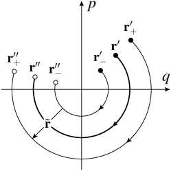
Figure 1: For an undamped harmonic oscillator, the pairs of phase-space trajectories $\mathbf{r}_{\pm}$ as well as their sum trajectory $\mathbf{r}$ satisfy the classical equations of motion. $\mathbf{r}^{\prime}_{\pm},\mathbf{r}^{\prime}$ and $\mathbf{r}^{\prime\prime}_{\pm},\mathbf{r}^{\prime\prime}$ denote the initial and final phase-space points of the trajectories, respectively, and $\tilde{\mathbf{r}}=\mathbf{r}_{+}-\mathbf{r}_{-}$.

As we shall see in Sect. 5, the relevant trajectories will be different for the harmonic oscillator in the presence of damping. While the mean of a trajectory pair still satisfies the classical equation of motion, the two trajectories themselves will behave nonclassically and separate exponentially fast in time. How this comes about will be explained in the following sections.

3 Influence functional theory

We now turn the so far isolated quantum system S into a dissipative quantum system by coupling it to a heat bath characterized by a temperature $T$. The complete Hamiltonian then is of the general form

$${\hat{H}}={\hat{H}}_{\mathrm{S}}+{\hat{H}}_{\mathrm{B}}+{\hat{H}}_{\mathrm{SB}}\,,$$ (18)

where the second and third term describe the bath Hamiltonian and the system-bath coupling, respectively.

As long as the complete Hilbert space is retained, the evolution of the density matrix is still of the form (2) where the system density operator $\hat{\rho}_{\mathrm{S}}$ is replaced by the full density operator $\hat{\rho}$. Correspondingly, in the time evolution operator (1) the system Hamiltonian has to be replaced by the full Hamiltonian (18). In position representation, (3) still holds with the appropriate replacements. In particular the coordinates are now $\mathcal{Q}=\{q,\mathbf{Q}\}$ and comprise the system coordinate $q$ as well as the vector of bath coordinates $\mathbf{Q}$.

If one considers a harmonic oscillator bilinearly coupled to a bath of oscillators [19], a situation which we will discuss in detail below, the Wigner propagator

$$G_{\rm W}({\bf\mathcal{R}}^{\prime\prime},{\bf\mathcal{R}}^{\prime},t)=\delta\left[{\bf\mathcal{R}}^{\prime\prime}-{\bf\mathcal{R}}^{\rm cl}({\bf\mathcal{R}}^{\prime},t)\right].$$ (19)

can be exactly expressed in terms of the classical phase-space trajectories $\mathcal{R}=\{\mathbf{r},\mathbf{R}\}$ of system and heat bath. They are obtained even in the continuum limit and for a thermal initial state of the bath by transforming to normal modes of the total system [20]. It is only after tracing out the heat bath that quantum effects come into play in the time evolution of the Wigner function. Instead of carrying out this analysis in phase space, we will rather follow the strategy presented in Sect. 2 for the undamped case where we started from the position-space description.

For a dissipative system, one is usually not interested in the full dynamics but only in the reduced dynamics of the system degree of freedom. In order to integrate out the bath degrees of freedom, one needs to specify the initial density matrix of system and bath. For simplicity, in the main part of the paper we will restrict ourselves to factorizing initial conditions [21, 22]. Then, the initial density matrix

$$\hat{\rho}(0)=\hat{\rho}_{\mathrm{S}}(0)\frac{\exp(-\beta\hat{H}_{\mathrm{B}})}{Z_{\mathrm{B}}}$$ (20)

is given by the product of the initial density matrix $\hat{\rho}_{\mathrm{S}}(0)$ of the system and the thermal density matrix of the heat bath at inverse temperature $\beta=1/k_{\mathrm{B}}T$. $Z_{\mathrm{B}}$ denotes the partition function of the bath. As we will show in A, our reasoning can readily be generalized to a certain class of nonfactorizing initial conditions.

The time evolution of the initial state (20) is obtained as a generalization of the considerations in Sect. 2 by substituting the single system degree of freedom by the ensemble of system and bath degrees of freedom. In order to obtain the reduced dynamics of the system, one needs to trace out the environmental degrees of freedom. This can be done analytically if the heat bath is modelled by a set of harmonic oscillators with masses $m_{j}$ and frequencies $\omega_{j}$ whose coordinates are bilinearly coupled to the system coordinate. The Hamiltonian (18) then consists of the three contributions [23]

$${\hat{H}}_{\mathrm{S}} =\frac{{\hat{p}}^{2}}{2m}+V({\hat{q}})\,,$$ (21)

$${\hat{H}}_{\mathrm{B}} =\sum_{j=1}^{\infty}\left[\frac{1}{2m_{j}}{{\hat{P}}_{j}}^{2}+\frac{1}{2}m_{j}\omega_{j}^{2}{\hat{Q}}_{j}^{2}\right]\,,$$ (22)

$${\hat{H}}_{\mathrm{SB}} =-{\hat{q}}\sum_{j=1}^{\infty}c_{j}{\hat{Q}}_{j}+{\hat{q}}^{2}\sum_{j=1}^{\infty}\frac{c_{j}^{2}}{2m_{j}\omega_{j}^{2}}\,,$$ (23)

where $c_{j}$ are the coupling constants. The second term in (23) corrects a potential renormalization induced by the coupling of the system to the heat bath. It turns out that the microscopic details of the heat bath and its coupling to the system appear in the reduced system dynamics only through the spectral density of bath oscillators

$$I(\omega)=\pi\sum_{j=1}^{\infty}\frac{c_{j}^{2}}{2m_{j}\omega_{j}}\delta(\omega-\omega_{j})\,.$$ (24)

For later convenience, we introduce two quantities which depend on this spectral density. The friction kernel is defined as

$$\eta(t)=\frac{2}{\pi}\int_{0}^{\infty}\mathrm{d}\omega\frac{I(\omega)}{\omega}\cos(\omega t)$$ (25)

and the correlation function of the noise [24] induced by the coupling to the heat bath is given by

$$K(z)=\int_{0}^{\infty}\frac{\mathrm{d}\omega}{\pi}I(\omega)\frac{\mathrm{cosh}[\omega(\frac{1}{2}\hbar\beta-\mathrm{i}z)]}{\mathrm{sinh}(\hbar\beta\omega/2)}\,,$$ (26)

where $z$ is a generally complex time.

Tracing out the heat bath, one finds for the time evolution of the reduced density matrix of the system starting from the factorizing initial state (20) [21, 22]

$$\rho_{\rm S}(q_{+}^{\prime\prime},q_{-}^{\prime\prime},t)=\int\!\mathrm{d}q_{+}^{\prime}\,\mathrm{d}q_{-}^{\prime}J(q_{-}^{\prime\prime},q_{+}^{\prime\prime},t;q_{+}^{\prime},q_{-}^{\prime})\,\rho_{\mathrm{S}}(q_{+}^{\prime},q_{-}^{\prime},0)\,.$$ (27)

Here we have introduced the propagating function which can be expressed in terms of a path integral over the system degree of freedom as

$$J(q_{-}^{\prime\prime},q_{+}^{\prime\prime},t;q_{+}^{\prime},q_{-}^{\prime}) =\frac{1}{Z}\int{\cal D}q_{+}{\cal D}q_{-}$$ (28)

$$\times\exp\left\{\frac{\mathrm{i}}{\hbar}[S_{\rm S}(q_{+})-S_{\rm S}(q_{-})]\right\}{\cal F}(q_{+},q_{-})\,.$$

The partition function $Z$ appearing here is an effective partition function of the damped system defined as the ratio of the partition functions of system plus bath and of the heat bath alone. The influence of the heat bath in (28) is contained in the influence functional

$$\mathcal{F}(q_{+},q_{-})=\exp\left[-\frac{{1}}{\hbar}\Phi(q_{+},q_{-})\right]$$ (29)

with the exponent

$$\Phi[q_{+},q_{-}] =\int_{0}^{t}\mathrm{d}s\int_{0}^{s}\mathrm{d}u\,K^{\prime}(s-u)\big{[}q_{+}(s)-q_{-}(s)\big{]}$$ (30)

$$\hskip 65.04366pt\times\big{[}q_{+}(u)-q_{-}(u)\big{]}$$

$$\quad+\frac{\mathrm{i}}{2}\int_{0}^{t}\mathrm{d}s\int_{0}^{s}\mathrm{d}u\,\eta(s-u)\big{[}q_{+}(s)-q_{-}(s)\big{]}$$

$$\hskip 65.04366pt\times\big{[}\dot{q}_{+}(u)+\dot{q}_{-}(u)\big{]}$$

$$\quad+\frac{\mathrm{i}}{2}\big{[}q_{+}^{\prime}+q_{-}^{\prime}\big{]}\int_{0}^{t}\mathrm{d}s\,\big{[}q_{+}(s)-q_{-}(s)\big{]}\,.$$

The prime in the first line indicates that the real part of the noise correlation function (26) should be taken.

4 Quantum damped harmonic oscillator

While the results reviewed in the previous section are valid for a general system degree of freedom, we will now specifically consider a damped harmonic oscillator with

$$V(\hat{q})=\frac{m}{2}\omega_{0}^{2}\hat{q}^{2}\,.$$ (31)

In this way, we will be able to generalize the considerations of Sect. 2 concerning the relevant trajectories in phase space. At the same time, this prevents making direct use of semiclassical phase-space dynamics based on the van-Vleck approximation as in Refs. [10, 11], since this only applies to sufficiently anharmonic potentials.

As for the propagator in the undamped case, the path-integral expression for the propagating function (28) is evaluated by an expansion around the paths maximizing the complex action. The dependence on the initial and final coordinates is entirely determined by these paths while the fluctuations only yield a time-dependent prefactor. For a harmonic oscillator, the complex action in (28) is stationary for trajectories satisfying

$$m{\ddot{q}}_{\pm}(s)+m\omega_{0}^{2}q_{\pm}(s)\mp\frac{1}{2}\frac{{\rm d}}{{\rm d}s}\int_{s}^{t}{\rm d}u\,\eta(s-u)\big{[}q_{+}(u)-q_{-}(u)\big{]}$$ (32)

$$+\frac{1}{2}\frac{\rm d}{{\rm d}s}\int_{0}^{s}{\rm d}u\,\eta(s-u)\big{[}q_{+}(u)+q_{-}(u)\big{]}=$$

$$\hskip 43.36133pt{\rm i}\int_{0}^{t}{\rm d}uK^{\prime}(s-u)\big{[}q_{+}(u)-q_{-}(u)\big{]}\,.$$

As in the undamped case, the paths are subject to the boundary conditions $q_{\pm}(0)=q_{\pm}^{\prime}$ and $q_{\pm}(t)=q_{\pm}^{\prime\prime}$.

The two equations of motion (32) replace the equations of motion (11) obtained for the undamped case. As a consequence of the coupling to the heat bath, the equations of motion (32) now include damping terms depending on the friction kernel (25). In addition, an imaginary nonlocal force appears indicating the occurrence of decoherence. For linear systems, it turns out that the imaginary part of the trajectories does not need to be considered and that their real part is sufficient to obtain the propagating function [26, 25]. As we shall see in the sequel, neither of the two paths follows a classical equation of motion and their separation grows exponentially fast. This somewhat surprising behavior is a consequence of the coupling to the heat bath.

In order to make the discussion transparent, we now consider the special case of Ohmic damping in addition to the assumption of factorizing initial conditions and the restriction to the real part of the equations of motion. We thus set $I(\omega)=m\gamma\omega$ and $\gamma(t)=\eta(t)/m=2\gamma\delta(t)$, so that the equations of motion (32) reduce to [22]

$${\ddot{q}}_{\pm}+\omega_{0}^{2}q_{\pm}+\gamma{\dot{q}}_{\mp}=0\,,$$ (33)

where the damping term couples the trajectories $q_{+}$ and $q_{-}$. It is interesting to note that $\gamma q_{\mp}$ acts actually as a driving instead of a damping in the sense that the separation between trajectories grows exponentially (see Fig. 2). This can be seen more clearly by decoupling the two equations of motion, using sum, $q=(q_{+}+q_{-})/2$, and difference coordinates, $\tilde{q}=q_{+}-q_{-}$. The equations (33) then read

$$\ddot{q}+\gamma\dot{q}+\omega_{0}^{2}q =0$$ (34)

$$\ddot{\tilde{q}}-\gamma\dot{\tilde{q}}+\omega_{0}^{2}\tilde{q} =0\,.$$

As in the undamped case, the sum trajectory corresponding to the paths $q_{+}$ and $q_{-}$ obeys the classical equation of motion, which here takes a time-local form because we have assumed Ohmic damping. In contrast to the sum coordinate $q$ which decreases exponentially in time, the difference coordinate $\tilde{q}$ grows exponentially so that we obtain a hyperbolic dynamics in the $(q,\tilde{q})$-plane. As a consequence, the trajectories $q_{\pm}$ do not obey the classical damped equation of motion. The solutions of the equations of motion (34) read

$$q(s) =q^{\prime}\frac{G_{-}(t-s)}{G_{-}(t)}+q^{\prime\prime}\frac{G_{+}(s)}{G_{+}(t)}\,,$$ (35)

$$\tilde{q}(s) =\tilde{q}^{\prime}\frac{G_{+}(t-s)}{G_{+}(t)}+\tilde{q}^{\prime\prime}\frac{G_{-}(s)}{G_{-}(t)}\,,$$

where

$$G_{\pm}(t)=\frac{1}{\omega_{\mathrm{d}}}\exp\left(\mp\frac{\gamma}{2}t\right)\sin\left(\omega_{\mathrm{d}}t\right)$$ (36)

and $\omega_{\mathrm{d}}^{2}=\omega_{0}^{2}-\gamma^{2}/4$. We remark that by choosing appropriate functions $G(t)$, more general linear damped system like the parametrically driven damped harmonic oscillator [27, 28, 29] can be studied with solutions of the form (35).

We now return to the propagating function which was given in (28) in terms of a twofold path integral. It is instructive to decompose the exponent into two parts

$$S(\tilde{q}^{\prime\prime},q^{\prime\prime},t;\tilde{q}^{\prime},q^{\prime})=S_{1}+S_{2}\,,$$ (37)

where

$$S_{1}=m\left[(q^{\prime}\tilde{q}^{\prime}+q^{\prime\prime}\tilde{q}^{\prime\prime})\frac{\dot{G}_{+}(t)}{G_{+}(t)}-q^{\prime}\tilde{q}^{\prime\prime}\frac{1}{G_{-}(t)}-q^{\prime\prime}\tilde{q}^{\prime}\frac{1}{G_{+}(t)}\right]$$ (38)

is obtained by evaluating the action of the system degree of freedom along the trajectories given by (35) while

$$S_{2}=\frac{\mathrm{i}}{2}\int_{0}^{t}{\rm d}s\int_{0}^{t}{\rm d}u\,K^{\prime}(s-u)\tilde{q}(s)\tilde{q}(u)$$ (39)

arises from the influence functional (29), i.e. by the interaction of paths at different times through the coupling to the environment. The significance of this decomposition will become clear in the following section where we discuss the results of the present section from a phase-space point of view.

5 Quantum damped harmonic oscillator in phase space

The undamped time evolution (13) of the Wigner function can immediately be transferred to the dissipative case if we relate the Wigner propagating function to the propagating function by means of

$$G_{\mathrm{W}}(\mathbf{r}^{\prime\prime},\mathbf{r}^{\prime},t) =\frac{1}{2\pi\hbar}\int{\rm d}\tilde{q}^{\prime}{\rm d}\tilde{q}^{\prime\prime}\exp\left[\frac{{\rm i}}{\hbar}(p^{\prime}\tilde{q}^{\prime}-p^{\prime\prime}\tilde{q}^{\prime\prime})\right]$$ (40)

$$\hphantom{\frac{1}{2\pi\hbar}\int}\times J(\tilde{q}^{\prime\prime},q^{\prime\prime},t;\tilde{q}^{\prime},q^{\prime})\,,$$

where we recall that $\mathbf{r}=(p,q)$ is the phase-space vector. Inserting (4) valid for the unitary case into (40) one recovers expression (14) for the Wigner propagator. We continue to restrict ourselves to factorizing initial conditions but present in A the generalization of (40) to nonfactorizing initial conditions.

Before analyzing the Wigner propagating function for Ohmic damping, we discuss the decomposition (37) of the exponent of the propagating function. The contribution (38) is linear in the difference coordinates $\tilde{q}^{\prime}$ and $\tilde{q}^{\prime\prime}$. Performing the transformation (40), we therefore arrive at the Wigner propagating function

$$G_{\mathrm{W}}({\bf r}^{\prime\prime},{\bf r}^{\prime},t)=\delta\left[{\bf r}^{\prime\prime}-{\bf r}^{\rm cl}({\bf r}^{\prime},t)\right]\,,$$ (41)

where the classical phase-space trajectory

$$p^{\rm cl}(t) =\dot{G}_{+}(t)p^{\prime}+m\left\{\frac{[\dot{G}_{+}(t)]^{2}}{G_{+}(t)}-\frac{1}{G_{-}(t)}\right\}q^{\prime}$$ (42)

$$q^{\rm cl}(t) =\frac{G_{+}(t)}{m}p^{\prime}+\dot{G}_{+}(t)q^{\prime},$$

with $G_{\pm}(t)$ defined by (36) is now damped. While (42) satisfies $q^{\mathrm{cl}}(0)=q^{\prime}$ as expected, the initial momentum is given by $p^{\mathrm{cl}}(0)=p^{\prime}-m\gamma q^{\prime}$. This initial slip is typical for factorizing initial conditions [26, 30].

Employing the Wigner propagating function (41) amounts to adding a velocity-dependent force in the system Hamiltonian as was proposed by Caldirola and Kanai (see e.g. the review [31] for an account of this kind of phenomenological approach). However, the Wigner propagating function (41) accounts only for part of the exponent of the propagating function. The second contribution (39) is quadratic in the difference coordinate and limits their contributions. As a result, the delta function in (41) will be broadened into a Gaussian

$$G_{\mathrm{W}}({\bf r}^{\prime\prime},t;{\bf r}^{\prime})=\frac{m}{2\pi\hbar\Lambda(t)^{1/2}}\left|\frac{\dot{G}_{+}(t)}{G_{+}(t)}\right|\\ \times\exp\left\{-\frac{1}{2\hbar\Lambda(t)}\left[{\bf r}^{\prime\prime}-{\bf r}^{\rm cl}(t)\right]^{\rm T}\mathsf{\Sigma}\left[{\bf r}^{\prime\prime}-{\bf r}^{\rm cl}(t)\right]\right\},$$ (43)

whose center moves along the damped classical trajectory (42). The matrix appearing in the exponent is given by its components

$$\mathsf{\Sigma}_{11} =a(t)$$ (44)

$$\mathsf{\Sigma}_{12} =\mathsf{\Sigma}_{21}=-m\frac{\dot{G}_{+}(t)}{G_{+}(t)}\left[a(t)+b(t)\right]$$

$$\mathsf{\Sigma}_{22} =m^{2}\frac{[\dot{G}_{+}(t)]^{2}}{[G_{+}(t)]^{2}}\left[a(t)+2b(t)+c(t)\right]$$

and $\Lambda(t)=\det(\mathsf{\Sigma})/m^{2}=a(t)c(t)-b(t)^{2}$. The functions

$$a(t) =[\dot{G}_{+}(t)]^{2}\Psi(t,t)$$ (45)

$$b(t) =\dot{G}_{+}(t)G_{+}(t)\left.\frac{\partial\Psi(t,t^{\prime})}{\partial t}\right|_{t^{\prime}\nearrow t}$$

$$c(t) =[G_{+}(t)]^{2}\left.\frac{\partial^{2}\Psi(t,t^{\prime})}{\partial t\partial t^{\prime}}\right|_{t^{\prime}\nearrow t}$$

can all be expressed in terms of a single function

$$\Psi(t,t^{\prime})=\int_{0}^{t}{\rm d}s\int_{0}^{t^{\prime}}{\rm d}u\,K^{\prime}(s-u)\frac{G_{+}(t-s)}{G_{+}(t)}\frac{G_{+}(t^{\prime}-u)}{G_{+}(t^{\prime})}\,.$$ (46)

This function is completely determined by the thermal position autocorrelation function $\langle q(t)q(0)\rangle$ and its time derivatives. Explicit expressions are given in B and the interested reader may also want to consult Ref. [26] for further details.

The Gaussian form of the Wigner propagating function (43) is a consequence of the linearity of the harmonic oscillator damped by the coupling to a harmonic heat bath. A similar expression has therefore been found in the Markovian limit [32]. Similarly, as indicated in A, the result can be generalized to the case of nonfactorizing initial conditions. Again one would find a Gaussian Wigner propagating function.

From (40) it follows that pairs of trajectories $q_{\pm}$ satisfying the equations of motion (33) and leading to a sum trajectory connecting the initial phase-space point $\mathbf{r}^{\prime}$ to the end point $\mathbf{r}^{\prime\prime}$ contribute with a weight determined by (39). As discussed in the previous section, according to (33) these pairs do not obey the classical damped equation of motion. The same is true in phase space. The hyperbolic character of the solutions of (34) already contains all quantum effects that arise upon tracing out the heat bath. The equations of motion (33) can therefore be lifted to the phase space of the central oscillator by defining $p_{\pm}=\dot{q}_{\pm}/m$,

$$\dot{p}_{\pm} =-m\omega_{0}^{2}q_{\pm}-m\gamma\dot{q}_{\mp}$$ (47)

$$\dot{q}_{\pm} =\frac{p_{\pm}}{m}\,.$$

so that the sum trajectory follows the classical equation of motion of the damped harmonic oscillator. This result was also found by Ozorio and Brodier [12] for the Markovian case derived directly from the Lindblad master equation.

In Fig. 2 we depict the time evolution in phase space of two trajectories $q_{\pm}$ indicated by $+$ and $-$ together with the corresponding sum trajectory shown in black. Due to the damping, the sum trajectory for long times approaches the origin of phase space. The trajectories $q_{\pm}$ grow exponentially for long times and therefore clearly behave nonclassically. Although in Fig. 2 the paths $q_{+}$ and $q_{-}$ have started on the same side of the origin of phase space, for long times they are found opposite to each other. This is a consequence of their exponential growth and of the fact that their midpoint approaches the origin of phase space.

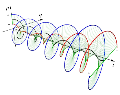
Figure 2: The time evolution of a pair of phase-space trajectories $\mathbf{r}_{\pm}$ marked by $+$ (depicted in blue) and by $-$ (depicted in red) is shown together with the corresponding classical sum trajectory depicted in black. While the sum trajectory decays to zero for long times, the trajectories $\mathbf{r}_{\pm}$ grow exponentially.

We close our discussion of the phase-space properties of the damped harmonic oscillator by considering how the thermal equilibrium state is approached for long times. First, we notice that in the Wigner propagator (43) the dependence on the initial phase-space coordinates $\mathbf{r}^{\prime}$ disappears in that limit because the sum coordinate then approaches the origin of phase space. Furthermore, the long-time behavior of the functions (45) is given by

$$a(t) \sim\frac{m^{2}}{\hbar}\frac{[\dot{G}_{+}(t)]^{2}}{[G_{+}(t)]^{2}}\langle q^{2}\rangle$$ (48)

$$b(t) \sim-\frac{m^{2}}{\hbar}\frac{[\dot{G}_{+}(t)]^{2}}{[G_{+}(t)]^{2}}\langle q^{2}\rangle$$

$$c(t) \sim\frac{\langle p^{2}\rangle}{\hbar}+\frac{m^{2}}{\hbar}\frac{[\dot{G}_{+}(t)]^{2}}{[G_{+}(t)]^{2}}\langle q^{2}\rangle\,,$$

where $\langle q^{2}\rangle$ and $\langle p^{2}\rangle$ are the second moments of position and momentum, respectively, in thermal equilibrium. Inserting these expressions into (43), one obtains the thermal Wigner function of the damped harmonic oscillator

$$W_{\beta}(p,q)=\frac{1}{2\pi(\langle q^{2}\rangle\langle p^{2}\rangle)^{1/2}}\exp\left(-\frac{p^{2}}{2\langle p^{2}\rangle}-\frac{q^{2}}{2\langle q^{2}\rangle}\right)\,.$$ (49)

In Fig. 3 we illustrate the time evolution of the Wigner propagating function for $\gamma=0.3\omega_{0}$ and $k_{\mathrm{B}}T=5\hbar\omega_{0}$ by means of an isosurface. The function (46) has been evaluated with the high-temperature approximation $K^{\prime}(t)=(2\gamma/\hbar\beta)\delta(t)$. The propagating function evolves from an initial delta function to the thermal Wigner function (49) which has a circular cross section because position and momentum are scaled with the square roots of the respective equilibrium second moments.

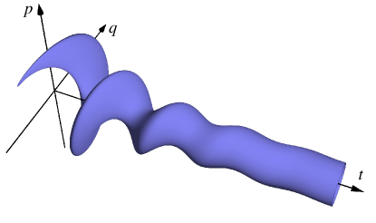
Figure 3: Isosurface of the time-dependent Wigner propagating function (43) for $\gamma/\omega_{0}=0.3$ and $k_{\mathrm{B}}T=5\hbar\omega_{0}$. Position and momentum are scaled with respect to the square root of the respective equilibrium second moments.

6 Conclusion

Our analysis of the propagating function of a damped harmonic oscillator in phase space has shown that pairs of trajectories contribute which, in contrast to the undamped case, are nonclassical in nature. In the course of time the distance between the two trajectories of a pair grows exponentially. This behavior is typical also for nonlinear systems [13] so that the damped harmonic oscillator can serve as an exactly solvable reference case. The harmonic oscillator coupled to a linear heat bath is however special insofar as the linearity of the system implies that the sum of the pairs of trajectories satisfies the classical damped equation of motion.

Furthermore, it was shown that it is the nonlocal interaction (39) appearing in a reduced description of the system degree of freedom which is responsible for the broadening of the delta-like Wigner propagator found for the undamped case into the Gaussian propagating function. While most of the explicit results have been presented for the special case of factorizing initial conditions, the generalization to a broader class of initial states is straightforward along the lines presented in A and the Gaussian nature of the propagating function remains unchanged.

Appendix A Propagating function for nonfactorizing initial conditions

In the main part of this paper, we have restricted our considerations to the case of factorizing initial conditions for the sake of simplicity. The generalization to nonfactorizing initial conditions is a bit more tedious but straightforward. In this appendix, we briefly derive the phase-space representation of the time evolution of a nonfactorizing initial Wigner function [33].

Specifically, we will consider nonfactorizing initial conditions where system and bath together are in their equilibrium state thus accounting for initial correlations. Then, operators taken from the Hilbert space of the system are allowed to act in order to generate a nonthermal initial state for the system. On the formal side, this preparation in comparison with factorizing initial conditions has two consequences. Firstly, in addition to the two real-time paths $q_{\pm}$, an imaginary-time path $\bar{q}$ appears. Secondly, a preparation function $\lambda(\tilde{q}^{\prime},q^{\prime},\bar{\tilde{q}},\bar{q})$ joins the real-time and imaginary-time paths. Here, $\bar{q}$ and $\bar{\tilde{q}}$ refer to sum and difference coordinates of the imaginary time path. The preparation function function describes the initial preparation and depends on the matrix elements of the system operators. For more details, we refer the reader to Ref. [26].

The generalization of (27) to the nonfactorizing initial conditions just described reads

$$\rho_{\rm S}(\tilde{q}^{\prime\prime},q^{\prime\prime},t) =\int\mathrm{d}\tilde{q}^{\prime}\mathrm{d}q^{\prime}\mathrm{d}\bar{\tilde{q}}\mathrm{d}\bar{q}\,J(\tilde{q}^{\prime\prime},q^{\prime\prime},t;\tilde{q}^{\prime},q^{\prime},{\bar{\tilde{q}}},{\bar{q}})$$ (50)

$$\hphantom{=\int}\times\lambda(\tilde{q}^{\prime},q^{\prime},{\bar{\tilde{q}}},{\bar{q}})\,.$$

Now, the propagating function also depends on the endpoints of the imaginary-time path. Introducing the Wigner transform of the preparation function

$$\lambda_{\mathrm{W}}(p^{\prime},q^{\prime},\bar{p},\bar{q}) =\frac{1}{(2\pi\hbar)^{2}}\int\mathrm{d}\tilde{q}^{\prime}\mathrm{d}\bar{\tilde{q}}\exp\left[\frac{\mathrm{i}}{\hbar}(\bar{p}\bar{\tilde{q}}-p^{\prime}\tilde{q}^{\prime})\right]$$ (51)

$$\hphantom{=\frac{1}{(2\pi\hbar)^{2}}\int}\times\lambda(\tilde{q}^{\prime},q^{\prime},\bar{\tilde{q}},\bar{q})\,,$$

we obtain for the time evolution of the Wigner function after carrying out the Fourier transform with respect to $\tilde{q}^{\prime\prime}$

$$W_{\mathrm{S}}(p^{\prime\prime},q^{\prime\prime}) =\int\mathrm{d}p^{\prime}\mathrm{d}q^{\prime}\mathrm{d}\bar{p}\mathrm{d}\bar{q}\,G_{\mathrm{W}}(p^{\prime\prime},q^{\prime\prime},t;p^{\prime},q^{\prime},\bar{p},\bar{q})$$ (52)

$$\hphantom{=\int}\times\lambda_{\mathrm{W}}(p^{\prime},q^{\prime},\bar{p},\bar{q})\,.$$

By comparison with (50) one finds for the relation between the propagating function introduced in (50) and its Wigner transform

$$G_{\mathrm{W}}(p^{\prime\prime},q^{\prime\prime},t;p^{\prime},q^{\prime},{\bar{p}},{\bar{q}}) =\frac{1}{2\pi\hbar}\int\mathrm{d}\tilde{q}^{\prime\prime}\mathrm{d}\tilde{q}^{\prime}\mathrm{d}\bar{\tilde{q}}$$ (53)

$$\times\exp\left[\frac{\mathrm{i}}{\hbar}(p^{\prime}\tilde{q}^{\prime}-p^{\prime\prime}\tilde{q}^{\prime\prime}-\bar{p}\bar{\tilde{q}})\right]J(\tilde{q}^{\prime\prime},q^{\prime\prime},t;\tilde{q}^{\prime},q^{\prime},\bar{\tilde{q}},\bar{q})\,.$$

For the special case of factorizing initial conditions, the coordinates $\bar{\tilde{q}}$, $\bar{q}$ and the momentum $\bar{q}$ are to be disregarded and one arrives at the relation (40) between the propagating functions in position and phase space.

Appendix B Propagating function and position autocorrelation function

The Gaussian nature of a harmonic oscillator coupled linearly to a bath of harmonic oscillators implies that its reduced dynamics can be expressed completely in terms of the thermal position autocorrelation function [34, 35]

$$C(t) =\langle q(t)q(0)\rangle=S(t)+\mathrm{i}A(t)$$ (54)

$$=\frac{\hbar}{\pi m}\int_{-\infty}^{+\infty}\mathrm{d}\omega\frac{\omega\hat{\gamma}(-\mathrm{i}\omega)}{(\omega^{2}-\omega_{0}^{2})^{2}+\omega^{2}\hat{\gamma}(-\mathrm{i}\omega)^{2}}\frac{\exp(-\mathrm{i}\omega t)}{1-\exp(-\beta\hbar\omega)}\,.$$

$S(t)$ and $A(t)$ denote the symmetrized and antisymmetrized correlation functions and correspond to the real and imaginary part of $C(t)$, respectively. $\hat{\gamma}(z)$ is the Laplace transform of the friction kernel (25) divided by the oscillator mass $m$. The antisymmetric correlation function is related to the function $G_{+}(t)$ introduced for the special case of Ohmic damping in (36) by

$$G_{+}(t)=-\frac{2m}{\hbar}A(t)\Theta(t)\,,$$ (55)

where $\Theta(t)$ is the unit step function. The second moments of position and momentum appearing in (49) are related to the symmetrized correlation function by $\langle q^{2}\rangle=S(0)$ and $\langle p^{2}\rangle=-m\ddot{S}(0)$, respectively. For the latter to be finite, the Laplace transform $\hat{\gamma}(z)$ requires a high-frequency cutoff.

The functions (45) are found to read [26]

$$a(t) =\frac{m^{2}}{\hbar}\frac{[\dot{G}_{+}(t)]^{2}}{[G_{+}(t)]^{2}}\left\{\langle q^{2}\rangle\left[1-\frac{[S(t)]^{2}}{\langle q^{2}\rangle^{2}}\right]+\frac{\langle p^{2}\rangle}{m^{2}}[G_{+}(t)]^{2}+2\dot{S}(t)G_{+}(t)\right\}$$ (56)

$$b(t) =-\frac{m^{2}}{\hbar}\frac{\dot{G}_{+}(t)}{G_{+}(t)}\left\{\langle q^{2}\rangle\left[1-\frac{[S(t)]^{2}}{\langle q^{2}\rangle^{2}}\right]\frac{\dot{G}_{+}(t)}{G_{+}(t)}+\dot{G}_{+}(t)\dot{S}(t)\right.$$

$$\hphantom{=-\frac{m^{2}}{\hbar}\frac{\dot{G}_{+}(t)}{G_{+}(t)}\Big{\{}}\left.-G_{+}(t)\ddot{S}(t)+\frac{S(t)\dot{S}(t)}{\langle q^{2}\rangle}\right\}$$

$$c(t) =\frac{m^{2}}{\hbar}\left\{\langle q^{2}\rangle\frac{[\dot{G}_{+}(t)]^{2}}{[G_{+}(t)]^{2}}+\frac{\langle p^{2}\rangle}{m^{2}}-\frac{1}{\langle q^{2}\rangle}\left[\dot{S}(t)-\frac{\dot{G}_{+}(t)}{G_{+}(t)}S(t)\right]^{2}\right\}\,.$$

If one takes into account that $G_{+}(t)$, $S(t)$, and their derivatives decay to zero for long times but not the ratio $\dot{G}_{+}(t)/G_{+}(t)$, one immediately finds the asymptotic expressions (48).

References

References

• [1] J. H. van Vleck, Proc. Natl. Acad. Sci. USA, 14 (1928) 178.
• [2] M. C. Gutzwiller, J. Math. Phys. 8 (1967) 1979.
• [3] M. C. Gutzwiller, J. Math. Phys. 12 (1971) 343.
• [4] P. Hänggi, P. Talkner, M. Borkovec, Rev. Mod. Phys. 62 (1990) 251.
• [5] P. Hänggi, W. Hontscha, Ber. Bunsenges. Phys. Chem. 95 (1991) 379.
• [6] M. V. Berry. Proc. R. Soc. Lond. A, 423 (1989) 219.
• [7] F. Toscano, M. A. M. de Aguiar, A. M. Ozorio de Almeida, Phys. Rev. Lett. 86 (2001) 59.
• [8] T. Dittrich, L. A. Pachón, Phys. Rev. Lett. 102 (2009) 150401.
• [9] P. P. de M. Rios, A. M. Ozorio de Almeida, J. Phys. A: Math. Gen. 35 (2002) 2609.
• [10] T. Dittrich, C. Viviescas, L. Sandoval, Phys. Rev. Lett. 96 (2006) 070403.
• [11] T. Dittrich, E. A. Gómez, L. A. Pachón, arXiv:0911.3871 (2009).
• [12] A. M. Ozorio de Almeida, P. de M. Rios, O. Brodier, J. Phys. A: Math. Theor. 42 (2009) 065306.
• [13] L. A. Pachón, T. Dittrich, G.-L. Ingold, in preparation.
• [14] R. P. Feynman, Rev. Mod. Phys. 20 (1948) 367.
• [15] R. P. Feynman, A. R. Hibbs, Quantum mechanics and path integrals, McGraw-Hill, New York, 1965.
• [16] M. Hillery, R. F. O’Connell, M. O. Scully, E. P. Wigner, Phys. Rep. 106 (1984) 121.
• [17] M. S. Marinov, Phys. Lett. A 153 (1991) 5.
• [18] N. L. Balazs, A. Voros, Ann. Phys. (N. Y.) 199 (1990) 123.
• [19] P. Ullersma, Physica 32 (1966) 27.
• [20] E. Pollak, J. Shao, D. H. Zhang, Phys. Rev. E 77 (2008) 021107.
• [21] R. P. Feynman, F. L. Vernon Jr., Ann. Phys. (N. Y.) 24 (1963) 118.
• [22] A. O. Caldeira, A. J. Leggett, Physica A 121 (1983) 587.
• [23] U. Weiss, Quantum Dissipative Systems, Series in Modern Condensed Matter Physics, vol. 13, World Scientific, Singapore, 2008.
• [24] P. Hänggi, G.-L. Ingold, Chaos 15 (2005) 026105.
• [25] V. Hakim, V. Ambegaokar, Phys. Rev. A 32 (1985) 423.
• [26] H. Grabert, P. Schramm, G.-L. Ingold, Phys. Rep. 168 (1988) 115.
• [27] C. Zerbe, P. Jung, P. Hänggi, Phys. Rev. E 49 (1994) 3626.
• [28] C. Zerbe, P. Hänggi, Phys. Rev. E 52 (1995) 1533.
• [29] S. Kohler, T. Dittrich, P. Hänggi, Phys. Rev. E 55 (1997) 300.
• [30] F. Haake, R. Reibold, Phys. Rev. A 32 (1985) 2462.
• [31] C.-I. Um, K.-H. Yeon, T. F. George, Phys. Rep. 362 (2002) 63.
• [32] O. Brodier, A. M. Ozorio de Almeida, Phys. Rev. E 69 (2004) 016204.
• [33] M. Merkl, Diploma thesis, Augsburg, 2006.
• [34] H. Grabert, U. Weiss, P. Talkner, Z. Phys. B 55 (1984) 87.
• [35] P. Riseborough, P. Hänggi, U. Weiss, Phys. Rev. A 31 (1985) 471.