Curvature in the color-magnitude relation but not in color$-\sigma$: Major dry mergers at $M_{*}>2\times 10^{11}M_{\odot}$?

Abstract

The color-magnitude relation of early-type galaxies differs slightly but significantly from a pure power-law, curving downwards at low and upwards at large luminosities ($M_{r}>-20.5$ and $M_{r}<-22.5$, respectively). This remains true of the color-size relation, and is even more apparent with stellar mass ($M_{*}<3\times 10^{10}M_{\odot}$ and $M_{*}>2\times 10^{11}M_{\odot}$, respectively). The upwards curvature at the massive end does not appear to be due to stellar population effects. In contrast, the color-$\sigma$ relation is well-described by a single power law. Since major dry mergers change neither the colors nor $\sigma$, but they do change masses and sizes, the clear features observed in the scaling relations with $M_{*}$, but not with $\sigma>150\,{\rm km~{}s}^{-1}$, suggest that $M_{*}>2\times 10^{11}M_{\odot}$ is the scale above which major dry mergers dominate the assembly history.

We discuss three models of the merger histories since $z\sim 1$ which are compatible with our measurements. In all three models, dry mergers are responsible for the flattening of the color-$M_{*}$ relation at $M_{*}>3\times 10^{10}M_{\odot}$ – wet mergers only matter at smaller masses. At $M_{*}>2\times 10^{11}M_{\odot}$, the merger histories in one model are dominated by major rather than minor dry mergers. In another, although both major and minor mergers occur at the high mass end, the minor mergers contribute primarily to the formation of the ICL, rather than to the stellar mass growth of the central massive galaxy. This model attributes the fact that $\alpha<1$ in the scaling $M_{*}\propto M_{\rm dyn}^{\alpha}$, to the formation of the ICL. A final model assumes that the bluest objects today were assembled by minor dry mergers of the bluest (early-type) objects at high redshift, whereas the reddest objects were assembled by a mix of major and minor dry mergers. In this model, the scatter of the color-magnitude relation should increase with redshift, and the dependence on environment should also be more pronounced at higher redshift: more clustered objects should be redder. Similar measurements of these relations at high redshift will provide further valuable constraints on the mass scale at which major dry mergers dominate the assembly history.

1 Introduction

The colors of early-type galaxies are tightly correlated with their luminosities (Sandage & Visvanathan 1978). The mean relation is well-described by a single-power law whose slope evolves little out to $z\sim 1$ (e.g. Kodama et al. 1998; Mei et al. 2009). This, and the small scatter around the mean relation, are thought to imply that the stellar populations in these objects are old (e.g. Bower et al. 1992; Bernardi et al. 2003b,c), although the total stellar metallicity, the $\alpha$-elements-to-iron abundance ratio, and light-weighted age, all increase along the relation (e.g. Bernardi et al. 2006; Gallazzi et al. 2006). Data sets are now large enough that significant departures from simple power laws can be detected: the mean color-magnitude relation appears to be steeper at faint luminosities (e.g. Baldry et al. 2004; Graham 2008; Skelton et al. 2009). This change in slope is thought to indicate that the mechanism by which the stars were assembled into a single object is different at low luminosities than at higher ones.

However, different morphological types define different color-magnitude relations. Since the mix of morphological types is a strong function of luminosity, it is possible that the observed curvature is really due to morphology, rather than to a change in formation histories at fixed morphology. Unfortunately, it is difficult to select large samples of a given morphological type that are pure. In what follows, we compare the color-magnitude relation obtained from a number of different ways of defining an early-type sample. We argue that while the steepening of the relation at faint luminosities may be affected by morphological effects, it appears to be present even in relatively pure samples of ellipticals – this may arise from the fact that dwarf and giant ellipticals are known to be different in other ways. However, we also show that, at the very highest luminosities, $M_{r}<-22.5$, the relation steepens again. In a companion paper, Bernardi et al. (2010b) show that this steepening occurs on the same scale where the size-luminosity and velocity dispersion-luminosity relations steepen and flatten, respectively (Bernardi et al. 2007). In addition, the trend for axis-ratio and color-gradient to increase with luminosity, reverse on this scale (Bernardi et al. 2008; Roche et al. 2010). When expressed in terms of stellar mass, the relevant scale is $M_{*}=2\times 10^{11}M_{\odot}$.

Section 2 describes the SDSS sample, and a number of ways for selecting early-types from it. Section 3 presents the associated color-magnitude relations, and shows that the trends we see are even more pronounced if we replace luminosity with stellar mass. It also shows that, in contrast, the color-$\sigma$ relation is well-described by a single power law over essentially the entire range of $\sigma$. Section 4 shows that the curvature is not due to stellar population effects. Section 5 compares our empirical results with simple models. While these toy models are not intended to provide a precise quantification of the color evolution, they provide a useful framework within which to discuss our measurements. A final section summarizes our findings, and discusses what they suggest about how the formation and assembly of early-type galaxies depend on mass and redshift.

Appendix A.1 describes a way of selecting early-types which exploits the fact that galaxy properties are approximately bimodal; Appendix A.2 contrasts this with selection based on eyeball classifications of morphology. A number of tests of systematics – robustness to changes in the scale on which rest-frame color is measured or inferred (color gradients and $k+e$ corrections) – are described in Appendix B. A final Appendix provides details of the expected changes to galaxy sizes and velocity dispersions if galaxy mergers occur along parabolic orbits and conserve mass and energy.

Where necessary we assume a flat background geometry that is dominated at the present time by a cosmological constant $\Lambda_{0}=1-\Omega_{0}$, where $\Omega_{0}=0.3$ is the background density in units of the critical density, with Hubble constant $H_{0}=70$ km s^-1Mpc^-1.

2 Sample

2.1 Data

In what follows, we will use the luminosities, colors, velocity dispersions and stellar masses of a magnitude limited sample of $\sim 250,000$ SDSS galaxies with $14.5<m_{\tt Pet}<17.5$ in the $r-$band, selected from 4681 deg² of sky. In this band, the absolute magnitude of the Sun is $M_{r,\odot}=4.67$.

We use the cmodel magnitudes as well as the Petrosian and model $g-r$ colors output by the SDSS database. The cmodel magnitude is a very crude disk+bulge magnitude which has been seeing-corrected. Rather than resulting from the best-fitting linear combination of an exponential disk and a deVaucouleur bulge, the cmodel magnitude comes from separately fitting exponential and deVaucouleur profiles to the image, and then combining these fits by finding that linear combination of them which best-fits the image (see Bernardi et al. 2010a for more discussion). The analysis which follows does not depend on whether one uses cmodel or Petrosian magnitudes. (Petrosian magnitudes are not seeing corrected, and they underestimate the total light in a deVaucouleurs profile by about 0.05 mags.)

However, choosing model rather than Petrosian colors does matter, because of color-gradients: the Petrosian color is associated with a larger scale, and so is typically bluer. For faint galaxies, the model colors have higher signal-to-noise ratio than do the Petrosian colors.

We apply $k$- and evolution-corrections to the luminosities and colors. We use $k$-corrections from Blanton & Roweis (2007), which are based on fitting templates to the observed colors. Because these are suspect at the bright end (Bernardi et al. 2010a argue that they assume younger stellar populations than may be realistic), we also explore spectral based $k$-corrections from Roche et al. (2009). Our evolution correction depends on the $k$-correction: we make high redshift objects fainter by $0.9z$ ($r-$band) and redder by $0.15z$ for Roche et al. $k$-corrections, and by $1.3z$ but with negligible color evolution correction for Blanton & Roweis. See Section B.1 and Figure 22 for more discussion.

We also use the concentration index $C_{r}$, which is the ratio of the scale which contains 90% of the Petrosian light in the $r$-band to that which contains 50%. Finally, we use the velocity dispersions and stellar masses of these objects as described in Bernardi et al. (2010a). The stellar masses were computed following Bell et al. (2003), who report that, at $z=0$, $\log_{10}(M_{*}/L_{r})_{0}=1.097\,(g-r)_{0}-0.406$, where the zero-point depends on the IMF (see their Appendix 2 and Table 7). We calibrate to a Chabrier IMF. (See Table 2 in Bernardi et al. 2010a for how to transform between different IMFs. Bernardi et al. also report a detailed comparison between the different ways of computing stellar masses and their biases – see their discussion of the stellar mass function and their Appendix A.) In Section 4 we make use of age and metallicity estimates for the objects in our sample. These come from Gallazzi et al. (2005), and are based on absorption line features in the spectra.

2.2 Sample selection

In this paper we are interested in early-type galaxies. The light profiles of such galaxies are more centrally concentrated, so they are expected to have larger values of $C_{r}$. Two values are in common use: a more conservative $C_{r}$$\geq 2.86$ (e.g. Nakamura et al. 2003; Shen et al. 2003) and a more cavalier $C_{r}$$\geq 2.6$ (e.g. Strateva et al. 2001; Kauffmann et al. 2003; Bell et al. 2003; Skelton et al. 2009). We can also select early-type galaxies following Hyde & Bernardi (2009), who use a combination of photometric features (a revised version of Bernardi et al. 2003a): i.e. fracDev $=1$ in $g$- and $r$-, $r$-band $b/a>0.6$ and log${}_{10}(r_{e,g}/r_{e,r})<0.15$. This last condition is essentially a cut on color gradient (Roche et al. 2010).

Recently, Bernardi et al. (2010a) have shown that requiring concentration indices $C_{r}\geq 2.6$ selects a mix in which E+S0+Sa’s account for about two-thirds of the objects; if $C_{r}\geq 2.86$ instead, then two-thirds of the sample comes from E+S0s; whereas Es alone account for more than two-thirds of a sample selected following Hyde & Bernardi (2009) (see Figures 11 and 12, and Table 3 of Bernardi et al. 2010a). E’s alone account for about 40%, 50% and 75% of the total stellar mass in samples selected in these three ways. In Appendix A.2, we also present results from a small subset of this dataset for which eye-ball classifications of morphology are available (from Fukugita et al. 2007).

There is a third method used to select early-type samples from the SDSS in addition to direct eye-ball classifications (e.g. Fukugita et al. 2007; Lintott et al. 2008) and to the two common automated ways introduced above (i.e. concentration index and Hyde–Bernardi). This is based on the fact that the color-magnitude relation is bimodal (e.g. Baldry et al. 2004; Blanton et al. 2005) at least out to redshifts of order unity (Willmer et al. 2006). This bimodality has sometimes been used as a simple way to select red sequence galaxies. Typically, one selects objects which lie redward of a straight color cut, or redward of a line which lies below, but parallel to, the red sequence (e.g. Zehavi et al. 2005; Blanton & Berlind 2007). The resulting sample is then treated as though it is comprised of early-types, even though it can contain a substantial fraction of edge-on spirals (Mitchell et al. 2005; Bernardi et al. 2010a). Although a cut on axis ratio can remove such objects (Bernardi et al. 2010a), this simple extra step is almost never taken.

We select a sample using ‘bimodality’ as follows. We first divide the full galaxy sample into narrow bins in luminosity. We then model the color distribution in each luminosity bin as the sum of two Gaussian components. The means and rms values of the two Gaussians, obtained by fitting the model to the data, give the red and blue sequences and their scatter; the amplitudes of the Gaussians give the fraction of galaxies in each component (e.g. Baldry et al. 2004; Skibba & Sheth 2009). Appendix A.1 provides details, and argues that the double-Gaussian decomposition correctly assigns the reddest objects at intermediate and low luminosities to the blue sequence. The means and rms of the two Gaussians and the fraction of galaxies in each component are listed in Table 2.

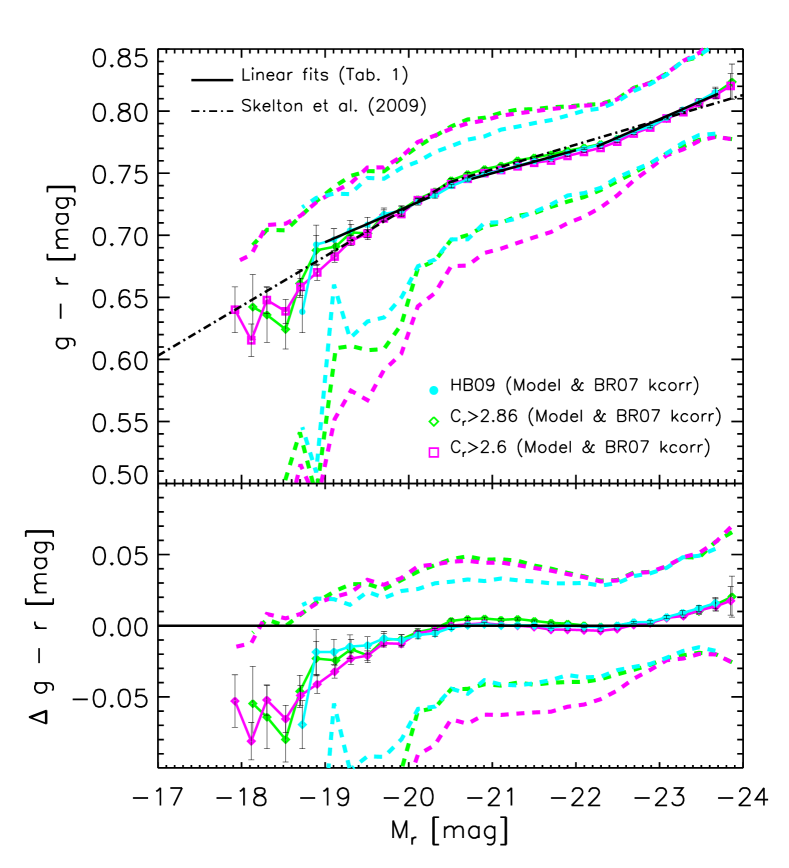
Figure 1: Red sequence defined by various samples (as labeled) when model colors and cmodel magnitudes are used and the $k$-correction is from Blanton & Roweis (2007). Top: Symbols with error bars show the mean $g-r$ for bins in $M_{r}$, and dashed lines show the rms scatter around this mean, for the different samples. Thick solid lines show the three regimes (fits are reported in Table 1) in the sample which is selected following Hyde & Bernardi (2009). Dot-dashed lines show the steep and shallow slopes for the faint and bright ends of this relation measured by Skelton et al. (2009) on a sample selected with $C_{r}>2.6$ and at $z<0.06$. Bottom: Same as top, except now, to reduce the dynamic range, a mean trend has been subtracted from the colors. Plot shows $g-r-(0.361-0.019\,M_{r})$ versus $M_{r}$: the reduction in dynamic range highlights the curvature in the relation.

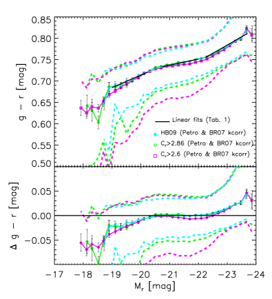
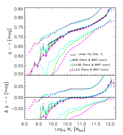
Figure 2: Red sequence defined by various samples (as labeled) when Petrosian colors and magnitudes are used and the $k$-correction is from Blanton & Roweis (2007). Top left: Symbols with error bars show the mean $g-r$ for bins in $M_{r}$, and dashed lines show the rms scatter around this mean, for the different samples. Thick solid lines show the three regimes (fits are reported in Table 1) in the sample which is selected following Hyde & Bernardi (2009). Bottom left: Same as top panel, except now, to reduce the dynamic range, a mean trend has been subtracted from the colors. Plot shows $g-r-(0.434-0.014\,M_{r})$ versus $M_{r}$: the reduction in dynamic range highlights the curvature in the relation. Top right panel shows a similar analysis of $\langle g-r|M_{*}\rangle$, where colors and stellar masses are derived from Petrosian quantities. The bottom right panel shows $g-r-(0.303+0.040\log_{10}M_{*}/M_{\odot})$ versus $M_{*}$.

3 Curvature

3.1 Curvature in the red sequence

Figure 1 shows that the different ways of selecting early-type samples mentioned above (cuts in $C_{r}$, or following Hyde & Bernardi 2009) produce almost indistinguishable color-magnitude relations. This is remarkable, given that the mean relation they define is not a simple power law. Rather, it bends downward at low luminosities, and upward at high luminosities, while being relatively flat at intermediate luminosities. The changes in slope occur around $M_{r}=-20.5$ and $M_{r}=-22.5$ mags. Table 1 quantifies the slopes.

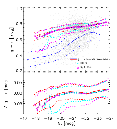
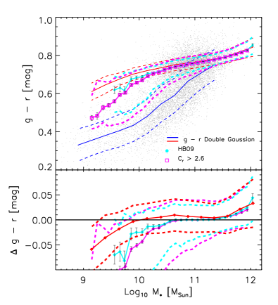
Figure 3: Dependence of the red sequence on how it is defined. Panel on the left shows the color-magnitude relation; panel on the right shows the color-$M_{*}$ relation. To highlight the curvature in the upper panels, bottom panels show the result of removing a linear trend: $g-r-(0.361-0.019M_{r})$ vs $M_{r}$ and $g-r-(0.224+0.049\log_{10}M_{*}/M_{\odot})$ vs $M_{*}$. Small dots show a representative subsample of the galaxies when model colors and cmodel magnitudes are used and the $k$-correction is from Blanton & Roweis (2007). Solid red and blue curves show the result of our double-Gaussian decomposition (see Table 2 in Appendix A.1); filled cyan circles show the color-magnitude relation for a sample selected following Hyde & Bernardi (2009); open magenta squares show this relation for objects with $C_{r}>2.6$. Dashed lines show the rms scatter around the mean relations. The relation found by the double-Gaussian fit is narrower and almost independent of $M_{r}$; the sample with $C_{r}>2.6$ has the largest scatter, particularly at $M_{r}>-20$.

The flattening of the slope as one moves brightwards from the faintest luminosities is in excellent agreement with that reported by Skelton et al. (2009) who selected galaxies with $C_{r}>2.6$ and at $z<0.06$. The dot-dashed lines show the relations they reported. Note, however, that they did not report any upward curvature at the brightest end. This may be because their sample was restricted to small redshifts ($z<0.06$), so they had many fewer objects at $M_{r}<-23$. As a result, at the bright end, our measurements zig-zag around their relation.

While our primary interest is in the fact that the relation is curved, notice that the samples do have different amounts of scatter around the mean relation: whereas they have similar red envelopes, the scatter bluewards tends to increase dramatically at faint luminosities, with the effect being most pronounced in the $C_{r}>2.6$ sample. Some of this is because, at fainter luminosities, these samples are increasingly contaminated by later-type galaxies (Bernardi et al. 2010a), so one might worry that the steeper slope at the faint end is due, at least in part, to this contamination. In Appendix A.2, we present a direct measurement of the color-magnitude relation in (substantially smaller) subsamples of fixed morphological type. This shows that there are three distinct regimes in a sample composed only of Es.

Table 1: Coefficients of linear fits to the $\langle g-r|M_{r}\rangle$ and $\langle g-r|M_{*}\rangle$ relations in the Hyde & Bernardi (2009) sample, where $g-r$ was computed using the Blanton & Roweis (2007) $k$-correction.

	PETROSIAN
Range	slope	z.p.
$-20.25<$M${}_{r}<-19$	$-0.029\pm 0.003$	$0.131\pm 0.051$
$-22<$M${}_{r}<-20.75$	$-0.014\pm 0.001$	$0.434\pm 0.012$
$-23.5<$M${}_{r}<-22.25$	$-0.039\pm 0.003$	$-0.104\pm 0.061$
$9.8<{\rm Log}_{10}{\rm M}_{*}<10.2$	$0.092\pm 0.012$	$-0.249\pm 0.072$
$10.5<{\rm Log}_{10}{\rm M}_{*}<11.1$	$0.040\pm 0.003$	$0.303\pm 0.028$
$11.4<{\rm Log}_{10}{\rm M}_{*}<11.9$	$0.094\pm 0.002$	$-0.305\pm 0.027$
	MODEL
Range	slope	z.p.
$-20.25<$M${}_{r}<-19$	$-0.029\pm 0.002$	$0.144\pm 0.024$
$-22<$M${}_{r}<-20.75$	$-0.019\pm 0.001$	$0.361\pm 0.013$
$-23.5<$M${}_{r}<-22.25$	$-0.029\pm 0.001$	$0.119\pm 0.027$
$9.8<{\rm Log}_{10}{\rm M}_{*}<10.2$	$0.090\pm 0.009$	$-0.215\pm 0.093$
$10.5<{\rm Log}_{10}{\rm M}_{*}<11.1$	$0.049\pm 0.001$	$0.224\pm 0.021$
$11.4<{\rm Log}_{10}{\rm M}_{*}<11.9$	$0.088\pm 0.006$	$-0.221\pm 0.065$

The left hand panel of Figure 2 shows that the curvature does not depend on precisely how the colors and magnitudes were defined: using Petrosian rather than model colors and magnitudes makes little difference. Appendix B shows that the small differences between model and Petrosian based quantities arise because model colors probe smaller scales than do Petrosian colors, and early-type galaxies have color gradients. It also shows that the appearance of three regimes is robust against changes in the $k+e$ corrections.

Since Petrosian colors probe more of the total light, we will use them, primarily, in what follows. The right hand panel of Figure 2 shows that the three regimes are even more pronounced if one replaces luminosity with stellar mass. This is easily understood: $\log M_{*}$ is obtained from $\log L$ by adding $1.097\,(g-r)-0.406$. So, to make this plot, one slides the reddest objects in the previous plot to the right, and the bluest to the left. Table 1 shows that the slope at intermediate masses is a factor of two shallower than at either end. The changes in slope occur at $M_{*}=3\times 10^{10}M_{\odot}$ and $M_{*}=2\times 10^{11}M_{\odot}$.

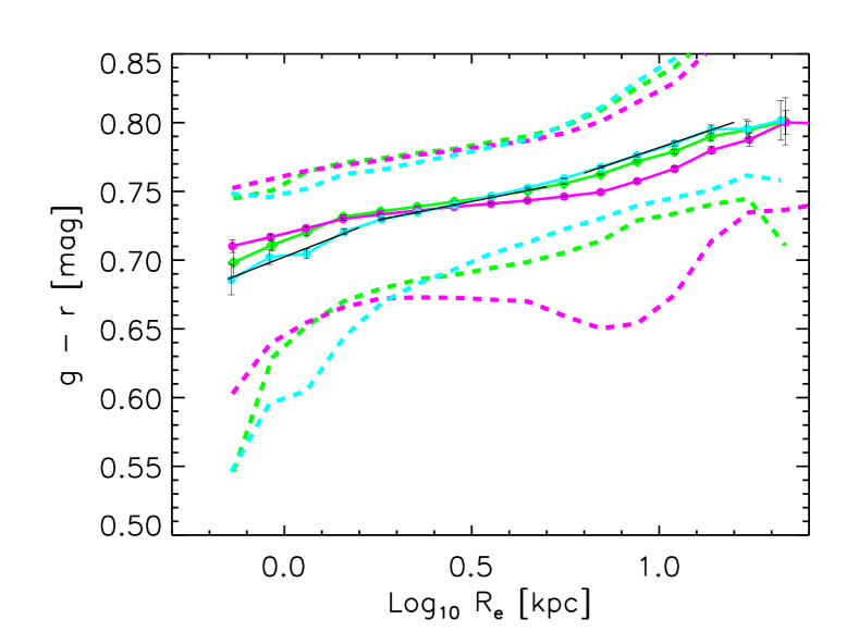
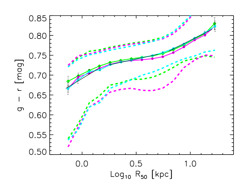
Figure 4: Petrosian color vs size, cmodel $R_{e}$ (top) and Petrosian ${\tt R_{50}}$ (bottom), for the three ways of selecting early-type samples (compare Figure 2).

Figure 3 displays the red and blue sequences defined by our double-Gaussian fits described in Appendix A.1 (the parameters are reported in Table 2). Clearly, the red sequence defined in this way also shows three regimes. Notice that the red sequence is considerably straighter and narrower than the blue, and that the thickness of the two sequences is almost independent of luminosity, even though this was not required during the fitting procedure. This is significant, because we were previously concerned that the bluewards flaring in the other samples might be signalling that the mean relation had been affected. Here, that argument cannot be made. Nevertheless, the mean red sequence is curved, in excellent agreement with that shown in Figure 2. The panel on the right shows that the three regimes are also present if one replaces luminosity with stellar mass. Table 3 provides details of the double-Gaussian fits to the associated red and blue sequences.

Before moving on, it is worth noting that the double-Gaussian fits do not fare well over the range $-18.5\geq M_{r}\geq-20.5$ (see Figure 13). At these luminosities, there appears to be a set of objects which populate the ‘green valley’ between the red and blue sequences. However, this third component is most needed at luminosities which lie below those where the color-magnitude relation flattens. So our neglect of, or contamination by this component is not to blame for the flattening at intermediate luminosities, nor for the steepening at the highest luminosities.

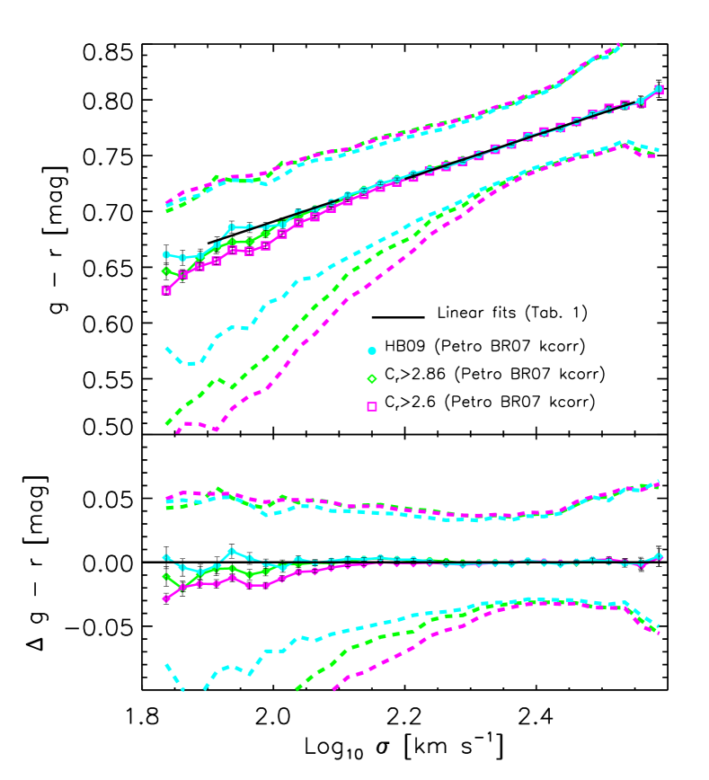
Figure 5: Petrosian color vs velocity dispersion for the three ways of selecting early-type samples (compare Figures 2 and 4).

3.2 Curvature in the color-$R$ and $M_{\rm dyn}$ relations but little in color-$\sigma$

In contrast to the previous two correlations with color, the color-size relation has been much less studied. Figure 4 shows that the color-$R$ relation also shows three distinct regimes. These are somewhat more obvious if we use Petrosian ${\tt R_{50}}$ than cmodel $R_{e}$. Three distinct regimes are also seen if the dynamical mass is used instead of stellar mass, although the curvature at the high-mass end is less steep (we have chosen to not show this plot).

In contrast to these relations which are rather curved, the color-$\sigma$ relation is rather well described by a single power law. This is shown in Figure 5. At large $\sigma$, the relation is independent of how the sample was selected. However, at $\log_{10}(\sigma/{\rm km~{}s}^{-1})<2.1$, samples which are more likely to include later types fall below the relation, suggesting that it is the changing morphological mix which is driving the curvature at small $\sigma$. Since major mergers are expected to change the mass and size of a galaxy while leaving $\sigma$ unchanged, the lack of curvature at large $\sigma$ is suggestive. We return to this in Sections 5 and 6.

Before moving on, we note that, for the bulk of the early-type population, the color-magnitude relation is a consequence of the color$-\sigma$ and $\sigma-$magnitude relations (Bernardi et al. 2005). This means that $\sigma$ determines both the color and the luminosity of an object, at least for the bulk of the population at lower luminosities. Now, the $\sigma-$magnitude relation flattens at large luminosities (Bernardi et al. 2007), and there is no curvature in the color-$\sigma$ relation (Figure 5). Hence, if there were no scatter around these relations, we would expect the color-magnitude relation to flatten rather than steepen at $M_{r}<-22.5$. Therefore, either $\sigma$ is no longer the important parameter at these high luminosities (and stellar masses), or the scatter around these relations is important.

4 Dependence on age and metallicity of the population

The previous subsections showed that the curvature in the color-magnitude relation is clearly seen in a number of other scaling relations with luminosity or stellar mass, but is essentially absent in correlations with $\sigma$. We now turn to a study of how the curvature depends on the age and metallicity of the population. Gallazzi et al. (2006) have shown that both age and metallicity increase along the color-$M_{*}$ relation. Here, our primary interest is in seeing if the curvature we have found is associated with stellar population effects.

Our age and metallicity estimates come from Gallazzi et al. (2005); they are based on absorption line features in the spectra. About 50 percent of our sample has ages between 8 and 10 Gyrs; 20 percent have ages between 10 and 12 Gyrs and only a percent are older than 12 Gyrs; 20 percent have ages between 6 and 8 Gyrs, and about 7 percent are younger than 6 Gyrs. Figure 6 shows that, although both age and metallicity tend to increase with mass, at fixed $M_{*}$, age and metallicity are anti-correlated: older galaxies are more metal poor, in agreement with previous work (Trager et al. 2000; Bernardi et al. 2005).

The top panel of Figure 7 shows that, at fixed metallicity and age, the color-magnitude relation is flat for galaxies with $M_{r}>-22.5$. The Figure actually shows results for metallicities between $1.25-1.6Z_{\odot}$. At smaller metallicity (not shown), the colors for the same age bins are offset blueward with respect to those shown here, but the color-magnitude relation remains flat. (This is because colors suffer from an age-metallicity degeneracy; Gallazzi et al. used spectral line indices to break this degeneracy.) In fact, the relation is flat whatever the age or metallicity. The middle panel shows this is true for the color-$M_{*}$ relation (at $\log_{10}M_{*}/M_{\odot}<11$) as well.

However, the color increases with luminosity (top) and even more strongly with $M_{*}$ (middle), at the most massive end which is dominated by the oldest galaxies. For younger galaxies, the upturn may be due to correlated errors in the $M_{*}$ and age estimates, but this is not a concern for the older objects (see Bernardi 2009 for more discussion).

This upwards curvature is not seen in the color-$\sigma$ relation (bottom). The slight increase of $g-r$ with $\sigma$, at fixed age and metallicity, may be due in part to the fact that the model estimates assume that all galaxies have the same ratio of $\alpha$-elements with respect to Fe. (Models which account for variations in $\alpha$-abundance are only just becoming available – they were not available to Gallazzi et al.) However, this ratio is known to be strongly correlated with $\sigma$: large $\sigma$ galaxies are $\alpha$-enhanced (Trager et al. 2000; Bernardi et al. 2005). Thus, while it may be that the results shown in the bottom panel are biased because this correlation has been ignored, it is extremely unlikely that the upwards curvature in the other two correlations (at fixed age and metallicity) is due to $\alpha$-enhancement related biases.

Figure 6: Age-metallicity relation for a number of bins in stellar mass. Although more massive objects are older and more metal rich, at fixed mass, older objects are more metal poor.

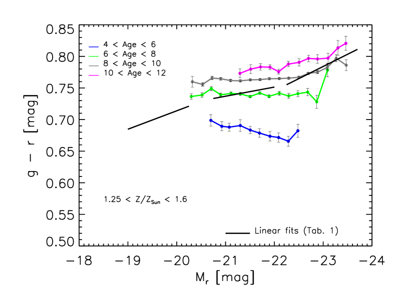
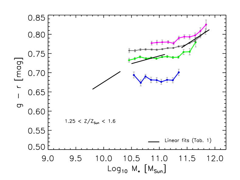
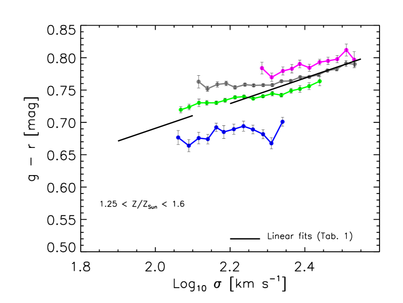
Figure 7: Color-magnitude, $M_{*}$ and $\sigma$ relations for galaxies with fixed age and metallicity (as indicated). Curvature in the top two panels is seen only for the oldest, most massive objects.

It is interesting that this same age and stellar mass scale is seen in recent studies of the $R_{e}-M_{*}$ relation. Shankar & Bernardi (2009) show that, at $M_{*}<2\times 10^{11}M_{\odot}$, older early-types tend to have smaller sizes than younger ones, perhaps because they formed at higher redshift from more dissipative mergers. However, at higher masses, this dependence on formation time disappears. Shankar & Bernardi suggest that this is because some later process has erased the trend. Although it is possible that some process decreases the sizes of younger early-types, Shankar & Bernardi focus on the possibility that the sizes of the older ones have increased (see also Shankar et al. 2010a). They argue that if older objects have undergone more dry mergers than their younger counterparts (of the same mass), then this would puff up their sizes, effectively erasing the trend which derives from formation age/time.

5 Dry merger models

In this section we are particularly interested in assessing if a late, dry merger-driven evolution for massive and passive early-type galaxies, is consistent with the measurements presented earlier in this paper.

Semi-analytic galaxy formation models make predictions for the curvature and evolution of the color-magnitude relation, so, in principle, they could be used to address this question. However, Bernardi et al. (2007) have shown that the red-sequence in these models is too red, and although it turns blueward at intermediate luminosities, it does not turn redward at the highest luminosities. In addition, Shankar et al. (2010a,b) have shown that the bulge sizes in some models could be somewhat discrepant with measurements.

Therefore, we now discuss a number of plausible scenarios in light of our measurements, some of which we simulate numerically. These are toy models: they do not provide a precise quantification of the color evolution. In what follows, we will assume that after some sufficiently large redshift, which we will take to be $z\sim 1$, the stars evolve passively, and this evolution is not differential. The absence of differential evolution means that we can effectively remove its effects from the following discussion, as including it simply results in an overall translation of the objects in the color-magnitude plane, but does not alter any features in the color-magnitude relation. To the extent that differential evolution is expected, it goes contrary to the trend that we observe: the most massive objects are expected to contain the oldest stars, so their luminosities and colors are expected to evolve more slowly than those of the least massive objects. Hence, while differential evolution may contribute to the flattening of the color-magnitude relation at intermediate luminosities, it seems an unlikely explanation for the steepening towards redder colors at large $M_{*}$.

Finally, we note that all the models we describe below assume that objects which are on the blue sequence at $z=1$, but evolve on to the red sequence as their gas supply is removed or exhausted – i.e., no mergers are involved – are either a negligible fraction of the population or, when they join the red sequence, they do so with colors that are representative of the red population for their mass (e.g., they are not biased bluewards), and they then evolve via dry mergers similarly to the other objects that were already on the red sequence. This assumption is consistent with the recent results of Peng et al. (2010) (see their Fig. 13 and 16) and Eliche-Moral et al. (2010) (who suggest that $z\sim 0.8$ might be more appropriate).

5.1 Similar initial conditions, but two types of merger histories (Model I)

Suppose that at some sufficiently high redshift (which we will take to be $z\sim 1$), the color magnitude relation was approximately a power law, and that, thereafter, the stars evolve passively, and this evolution is not differential. Then, dry mergers will cause the color magnitude relation to curve bluewards (from the initial power law) at the bright end, with the amount of curvature depending on the typical mass ratio of the mergers, and how that ratio depends on mass. We will loosely refer to mass ratios of 0.3:1 or greater as being major mergers, and smaller ratios as being minor.

Suppose that objects which are low mass today were assembled from both minor and major mergers, whereas the most massive objects experienced only 1:1 mergers. Then, the color magnitude relation will be flattened from the initial power law at low luminosities (minor mergers make the merged product bluer), but it will simply be translated to the right at high luminosities. Figure 8 shows this schematically. By adjusting the total mass growth and ratios at low masses, and the mass scale at which the mergers become major only, this scheme can be made to agree with our measurements.

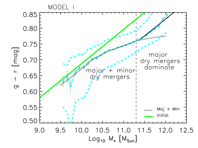
Figure 8: Origin of the color-$M_{*}$ relation if the stellar mass growth at $\log_{10}M_{*}/M_{\odot}>11.3$ is through major (1:1) dry mergers only. Such mergers translate the initial power-law relation (green solid line, here assumed to be for $z=1$) to the right (black solid line offset to right). Minor mergers at lower masses tend to flatten the relation from the initial power-law (dotted line), because the merger product must be bluer than its most massive progenitor. Given an initial relation (here assumed to be a power-law at $z=1$) the free parameters in this model are the mass scale at which 1:1 mergers dominate, the ratio of minor to major mergers at lower masses. Solid cyan line and associated error bars show the relation we see at $z\sim 0$; dashed lines show the rms spread around this mean relation.

In this model, the lack of curvature in the color-$\sigma$ relation can be understood as follows. The major 1:1 mergers will change neither $g-r$ nor $\sigma$, so they still lie on the initial relation. Minor mergers which decrease the color also decrease $\sigma$; this partially removes the flattening (in color-$\sigma$) which is so much more evident in the color-magnitude relation. Thus, in this model, the color-$\sigma$ relation at $z\sim 0$ differs from that at $z\sim 1$ primarily because of passive evolution of the colors – if the evolution is not differential, then the local relation is simply offset from that at higher $z$. In addition, whereas major mergers change the size proportionally to the mass, minor mergers change the sizes more than the masses. This accounts for the larger range in $R_{e}$ for which the color-$R_{e}$ slope is shallow.

It is worth stating explicitly that this model works because there is a color-magnitude relation at $z\sim 1$. Then, the additional requirement that the most massive galaxies are formed from major mergers, means that the most massive galaxies today formed from objects that were redder than those which make intermediate mass galaxies. Bernardi et al. (2007) noted that just such a conspiracy of mass/color-dependent mergers was required to explain the red colors of BCGs. Unfortunately, there is no obvious choice for the transition mass scale which plays a crucial role in this model, although, as we now argue, color gradients may hold an important clue.

In particular, Roche et al. (2010) show that color gradients are maximal at $M_{r}=-22$ (see our Figure 20). Whereas major mergers are expected to decrease color gradients, minor mergers should not change the gradients significantly, or they may enhance them slightly. This is because the smaller bluer object involved in the minor merger will deposit most of its stars at larger distances from the center of the object onto which it merged. Bernardi et al. (2010b) show that this same scale appears in other scaling relations as well. Thus, it may be that $M_{r}<-22$, which corresponds to $M_{*}>2\times 10^{11}M_{\odot}$, is the scale above which major mergers dominate.

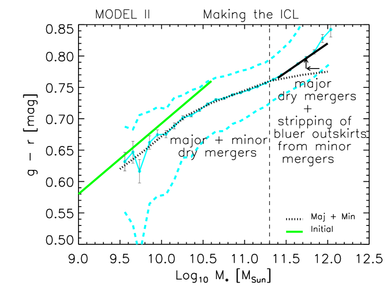
Figure 9: Origin of the color-$M_{*}$ relation if the stellar mass growth at the most massive end is through major dry mergers, because minor mergers (in this case, at $\log_{10}M/M_{\odot}>11.3$) contribute primarily to the ICL. Note that although these minor mergers will not change the stellar mass, they will affect the size and velocity dispersion (hence dynamical mass) of the merger product. Green solid line shows the relation we assume at $z=1$, dotted line shows the relation at $z=0$ due to minor mergers at lower masses, black solid line shows the $z=0$ relation at large $M_{*}$, where the minor mergers contribute to the ICL rather than to $M_{*}$, and solid cyan line with associated error bars and dashed lines (same as previous figure) show our $z\sim 0$ measurements.

5.2 Similar initial conditions, but inclusion of stripping/ICL (Model II)

This model is similar to the previous one, except that we assume that the massive end is dominated by objects in clusters, for which the effects of tidal stripping etc. matter (Figure 9). In this case, we assume that mergers at the high mass end may be both major and minor, but that sufficiently minor mergers do not actually contribute to the stellar mass of the final object, because they will be shredded; they contribute to the intercluster light. Note that minor mergers will produce changes in the size and velocity dispersion (hence dynamical mass) of the merger product, just not to the stellar mass. Thus, although the assembly history of BCG-like objects will involve both minor and major mergers, the stellar mass only grows in major mergers.

The net result will be similar to the previous model, with shallowing at low masses where both types of mergers happen (but stripping does not), and a parallel shift to larger masses of the initial (steeper) relation at the high luminosity end (where stripping erases the effects of minor mergers on the mass growth). I.e., in this model, the transition mass scale is related to the formation of the ICL.

Note that color gradients of the satellites which are stripped means that stars which do make it all the way to the central object will be redder, further steepening (or producing less flattenning of) the color-$M_{*}$ relation at the massive end. (If so, the ICL should be bluer than the BCG.) In addition, because some mass is lost to the ICL (some estimate that there is at least as much mass in the ICL as there is in the BCG), the color-magnitude relation will not extend to as high masses as in our first model. And finally, in this model, the ratio of stellar to dynamical mass should decrease at large masses, in qualitative agreement with the observation that $M_{*}\propto M_{\rm dyn}^{0.75}$. On the other hand, by consigning to the ICL some of the stellar mass that would otherwise have ended up in massive objects, this model is constrained by recent work suggesting that there is 50% more mass in objects with $\log_{10}M_{*}/M_{\odot}>11.3$ than previously thought (Bernardi et al. 2010b). This model must make such objects, as well as the ICL.

5.3 Correlation between color-magnitude residuals and mergers (Model III)

In this model, we distinguish between objects which lie redward of the mean color-magnitude relation at $z=1$, and those which lie blueward (Figure 10). Here, we assume that the redder objects are older, in agreement with the trend at $z=0$ (Kodama et al. 1998; Bernardi et al. 2005). We then assume that these redder objects were involved in major and minor mergers, whereas the bluer objects only experienced the most minor mergers, so they have increased their mass little since $z\sim 1$.

If our previous model of stripping which contributes to the formation of ICL (i.e. Model II) is realistic, then, in the present context, it would apply only to the redder objects. However, by ensuring that red objects merge with red ones, mergers in this model produce less of a decrease in slope, so less is required of processes like stripping to reproduce the turn up towards redder color at the high-mass (luminosity) end. Therefore, it may be easier for this model to produce the observed amount of stellar mass locked-up in objects with $\log_{10}M_{*}/M_{\odot}>11.2$ at $z\sim 0$.

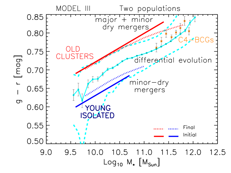
Figure 10: Origin of color-$M_{*}$ relation if the oldest objects at the present time formed from the oldest, reddest objects in the past, through a sequence of major and minor dry mergers, whereas the youngest objects today formed from minor mergers of bluer objects. Upper red solid line shows the assumed color-$M_{*}$ relation of the oldest objects at $z=1$; lower blue solid line shows that for the youngest objects at $z=1$. The associated dotted lines show how these relations have changed by $z=0$. Error bars and associated dashed lines (same as in previous Figure) show $\langle{\rm color}|M_{*}\rangle$ for the full sample at $z\sim 0$, and orange filled circles with error bars show this relation for BCGs at $z\sim 0$.

In many respects, this model is a variant of Model I. There, major mergers were used to ensure that the most massive objects formed by mergers of the reddest objects. The present model achieves this by assuming that massive objects are older, rather than making a specific assumption of major vs minor mergers. Additionally, here, the minor mergers which produce the lowest mass galaxies are preferentially of bluer objects, so they tend to result in bluer colors today. Thus, the conspiracy of mass/color-dependent mergers noted by Bernardi et al. (2007) to explain BCGs is here extended to the faint end as well. Note that, at the high mass end, this conspiracy may alleviate the tension between $\alpha$-enhancement ratios and late assembly models that has been emphasized by Pipino & Matteucci (2008).

In the previous models (i.e. Model I and II), the curvature is determined by the slope of the $z\sim 1$ color-magnitude relation: a flatter slope produces a smaller effect. Here, the scatter in the $z=1$ color-magnitude relation also matters: a smaller scatter also produces a smaller effect (e.g., if there were no scatter around the $z\sim 1$ relation, we would have no Model III).

It may help to think of the cluster population at $z=0$ as being made of these redder objects, whereas the bluer objects are now in lower density regions. This raises a potential problem because, at the present time, the environmental dependence of the color-magnitude relation of early-type galaxies is small (e.g. Bernardi et al. 2006). However, two effects in this model serve to help meet this constraint. First, the flattening and rightwards shift of the sequence defined by the older galaxies (red dotted line in Figure 10) brings it into better agreement with the relation defined by extrapolating the relation of the younger objects (blue solid line) to higher masses, thus reducing the offset in colors between cluster and field galaxies that would otherwise result. And second, differential evolution (because now we explicitly assume the populations have different ages) also acts to erase the offset in colors between the younger and older galaxies (which we have schematically represented by shifting the dotted blue line slightly redwards of the solid blue line). Together, both effects also make the scatter in the color-magnitude relation smaller at $z=0$ than at $z=1$. Note that, in addition to this testable prediction, this model also suggests that the residuals from the high redshift relation should correlate more strongly with environment than they do today. This is because, in this model, objects which are redder than average at $z\sim 1$ are in clusters at $z=0$ – but in hierarchical structure formation models, objects in clusters today were in overdense regions in the past (e.g. Mo & White 1996; Sheth 1998; Sheth et al. 2006).

Figure 11: Stellar mass versus velocity dispersion in the SDSS (filled symbols). Long-dashed line shows our assumed relation at $z=1$. The other curves show the result of evolving it down to redshift $z=0$, as detailed in the text, for three choices of $f_{\rm MIN}$.

5.4 Numerical implementation of Model I

To illustrate Model I, we have performed crude numerical simulations in which we prescribe the joint distribution of color, stellar mass and velocity dispersion at $z=1$. We then let these galaxies merge at the rate expected from observations and halo occupation modelling, always assuming zero-energy orbits with no energy dissipation. The assumption that both the initial objects and the final ones are in virial equilibrium allows one to determine the scaling relations of the population at late times from those of the initial population (see Appendix C for details). We then compare the resulting scaling relations with our measurements in the SDSS at $z=0$. Note that this approach assumes that objects which are on the blue sequence at $z=1$, but evolve on to the red sequence as their gas supply is removed or exhausted – i.e., no mergers are involved – are a negligible fraction of the population.

We set the scaling relations of the initial population as follows. We assume the color-$M_{*}$ relation has the same slope at $z=1$ as at $z=0$; this is consistent with observations (Mei et al. 2009). We then assume that the $\sigma-M_{*}$ relation at $z=1$ is the same power-law (both slope and zero-point) as the faint end of the $z=0$ relation. At $z=0$ the color-$M_{*}$ slope equals the product of the color-$\sigma$ and $\sigma-M_{*}$ slopes (Bernardi et al. 2005); we assume this is also true at $z=1$. So the one free parameter is the zero-point of the $z=1$ color-$M_{*}$ relation; setting it also determines the zero-point of the $z=1$ color-$\sigma$ relation. The low-$z$ dependence of the color-magnitude relation suggests that the $g-r$ colors are bluer at higher redshifts by approximately $0.2z$ (Figure 22). Therefore, we assume that they continue to evolve in this way upto $z=1$.

Figure 12: Same as Figure 11 but for the color-$M_{*}$ (top) and color-$\sigma$ (bottom) relations.

We then evolve the $z=1$ relations down to $z=0$ by a sequence of dry mergers. We do so by dividing the interval $0<z<1$ into ten discrete steps. For each, we estimate how the dry merger rate depends on stellar mass following Hopkins et al. (2010). This uses a convolution of the host halo merger rates with the average stellar-to-halo mass relation at each redshift, while also taking into account the gas fraction involved in each merger event (see Hopkins et al. 2010 for details, who provide a numerical algorithm to implement their model). The relevant merger rates are in broad agreement with a variety of direct observations (e.g Hopkins et al. 2010; Robaina et al. 2010 and references therein) and other theoretical estimates (e.g., Guo & White 2008). For consistency with the observed rather passive evolution characterizing the bulk of early-type galaxies (e.g Wake et al. 2008), we only consider dry mergers (with $f_{\rm gas}\leq 0.1$) as drivers of the late-time evolution. The exact threshold for $f_{\rm gas}$ does not change the overall trends discussed below.

The most important feature of these merger rates is that the evolutionary paths of the highest stellar mass bins are characterized by a larger number of major dry mergers. As we show below, this means that the colors of the objects which merge to make the most massive galaxies today are typically redder than those which make intermediate mass galaxies, whereas the more minor mergers which produce the lowest mass galaxies are preferentially of bluer objects, so they tend to result in bluer colors today. This is precisely the conspiracy of mass/color-dependent mergers the Bernardi et al. (2007) argued was required to explain the red colors of BCGs – our model quantifies the resulting trends.

The merger rates, and our results, depend on the mass ratio of the merging objects. If $m$ is the initial object in a given time step, then the merged object has mass $m(1+f)$. An object initially of mass $m_{0}$ and velocity dispersion $\sigma_{0}$, which undergoes $N$ zero-energy (sometimes called parabolic) dry mergers with other objects of mass $m_{i}<m_{0}$ and velocity dispersion $\sigma_{i}$, will result in an object of mass $M_{f}$ and velocity dispersion $\sigma_{f}$ which are given by

$$M_{f} = m_{0}\,(1+\sum_{i=1}^{N}f_{i})$$

$$\sigma_{f}^{2} = \sigma_{0}^{2}\,\frac{1+\sum_{i=1}^{N}f_{i}\,(\sigma_{i}/\sigma_{0})^{2}}{1+\sum_{i=1}^{N}f_{i}}\ ,$$ (1)

$$\frac{L_{r}}{L_{g}} = \frac{\sum_{i}L_{ri}}{\sum_{i}L_{gi}}=\frac{L_{r0}}{L_{g0}}\frac{1+\sum_{i}L_{ri}/L_{r0}}{1+\sum_{i}L_{gi}/L_{g0}}$$

$$= \frac{L_{r0}}{L_{g0}}\frac{1+\sum_{i}f_{i}(\Gamma_{r0}/\Gamma_{ri})}{1+\sum_{i}f_{i}(\Gamma_{r0}/\Gamma_{ri})(L_{r0}/L_{g0})/(L_{ri}/L_{gi})}$$

where $f_{i}\equiv m_{i}/m_{0}<1$ and $\Gamma_{r}\equiv(M_{*}/M_{\odot})/(L_{r}/L_{\odot})$. Since $(g-r)_{0}>(g-r)_{i}$, the expression above shows that the merger product $M_{f}$ would be bluer than $m_{0}$ if we were to ignore the aging of the stellar population. To simplify this expression for the color further, we assume that $\log\Gamma_{r}\propto 1.097\,(g-r)$ with a redshift dependent zero-point. Since our expression only involves ratios of $\Gamma_{r}$s, this zero-point cancels out, making

$$g-r = (g-r)_{0}+2.5\log_{10}\left(\frac{1+\sum_{i}f_{i}\,10^{1.097\,\Delta c_{i}}}{1+\sum_{i}f_{i}\,10^{1.497\,\Delta c_{i}}}\right)$$

$$\Delta c_{i} \equiv (g-r)_{0}-(g-r)_{i}.$$ (2)

In our analysis, we require $f>f_{\rm MIN}$, and we study how our results change as we increase $f_{\rm MIN}$. In practice, we divide the interval $0<z<1$ into a set of ten discrete time steps. For a given time bin, we pick three equally spaced bins of $f$ which satisfy $f_{\rm MIN}\leq f\leq 1$ (we show results for three choices of $f_{\rm MIN}$). For each bin of $f$ we first compute the mean number $N_{m}$ of expected dry mergers undergone by a galaxy of mass $m_{0}$ and velocity dispersion $\sigma_{0}$ with others of mass $m_{1}=fm_{0}$ and velocity dispersion $\sigma_{1}$, and then update mass, size, velocity dispersion and color according to the relations discussed above. After the mass-weighting update of the colors which results from the dry merger, we shift them redwards by $0.2(z_{j}-z_{j+1})$, where $z_{j}$ denotes the redshift associated with the time-bin just before the merger. We then iterate from $z=1$ down to 0. Notice that $\sigma_{0}<\sigma_{1}$ as $m_{0}>m_{1}$; if neither $f$ nor $N$ vary with $m_{0}$, then, at late times, the $\sigma-M$ relation shifts towards smaller $\sigma$ for a given $M$. In practice, since $fN$ increases with $M$, the downwards shift is larger for the most massive objects. This makes the $\sigma-M$ relation flatten at large $M$.

Figure 11 shows the $M_{*}-\sigma$ relation for three choices of $f_{\rm MIN}$: solid, dot-dashed, and dotted lines represent models with $f_{\rm MIN}=0.3,0.2,0.1$, respectively, while the long-dashed line shows the assumed $z=1$ relation. Figure 12 shows the associated changes to the color-$M_{*}$ and color-$\sigma$ relations. Notice that our dry merger models produce strong breaks in the $z=0$ color-$M_{*}$ relation while keeping the color-$\sigma$ relation closer to a power-law (bottom panel of Figures 12), in reasonable agreement with our measurements.

6 Discussion

Our study of the color-magnitude and color-$M_{*}$ scaling relations has revealed interesting trends: one at $M_{*}\sim 3\times 10^{10}M_{\odot}$ which had been noticed before (Kauffmann et al. 2003; Skelton et al. 2009), and another at high luminosities ($M_{r}\leq-22.5$) and masses ($\log_{10}(M_{*}/M_{\odot})\geq 11.3$), which is new to our work. These trends are qualitatively independent of exactly how the early-type sample is selected. In most cases, the (weak) dependence on precisely how the sample was selected can be traced to contamination of the red-sequence by edge-on spirals. In a related paper, Bernardi et al. (2010b) show that a number of other scaling relations also indicate that these luminosity and mass scales are special.

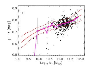
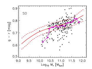
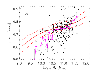
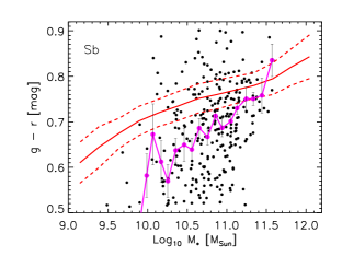
Figure 19: Same as Figure 18, but with luminosity replaced by stellar mass. Table 3 provides the parameters of the red sequence defined by double-Gaussian fits, shown here as the solid red line.

The red sequence is considerably straighter and narrower than the blue (Figure 3). However, it is not a simple power law: it is shallower between $-20.5>M_{r}>-22.5$ than at either the fainter or brighter ends (Figure 2 and Table 1). This curvature is not due to contamination by later morphological types at the faint end (Figure 18). It also does not depend on whether one uses Petrosian or model colors (Figure 20); although color-gradients mean that the scale on which the color is defined does lead to small quantitative differences. The curvature is also robust to (reasonable changes in) the choice of $k$-correction provided one properly accounts for evolution (Figure 22). Unless care is taken to account for it, this curvature may be confused with evolution in magnitude limited surveys (discussion following Figure 22). All these properties of the color-magnitude relation are also true of the color-stellar mass relation (Figures 2, 3, 19 and Tables 1 and 3), and the color-$R_{e}$ relation (Figure 4).

The curvature towards redder colors at the brightest ($M_{r}\leq-22.5$), most massive ($\log_{10}(M_{*}/M_{\odot})\geq 11.3$) end is evident at fixed age and metallicity, suggesting that it is not driven by stellar population effects (Figure 7). In contrast, the color-$\sigma$ relation shows no curvature at high $\sigma>150\,{\rm km~{}s}^{-1}$ (Figure 5). The fact that there is no feature at the largest $\sigma$, despite clear features in the scalings with $M_{*}$, has strong implications for models of the assembly histories of massive galaxies.

Skelton et al. (2009) have argued that the change from a steeper slope at low luminosities to a shallower one at $M_{r}<-20.5$ is due to a change in formation histories. They associate the shallower slope with recent major dry mergers which are expected to increase the luminosity and stellar mass without changing the color significantly. Since such mergers are expected to leave the velocity dispersion unchanged, that fact that there is no curvature in the color-$\sigma$ relation (Figure 5) seems in striking agreement with the dry major merger hypothesis. In addition, dry major mergers are expected to increase the size in proportion to the mass, and we do see some flattening in the color-$R_{e}$ relation (Figure 4). However, if the flattening at intermediate luminosities (and stellar masses, and sizes), with no curvature in the color-$\sigma$ relation is indeed due to major dry mergers, then it seems difficult for such a scenario to explain the steepening at even higher luminosities ($M_{r}<-22.5$ or $\log(M_{*}/M_{\odot})>11.3$), even though these are precisely the objects for which the dry merger hypothesis is most commonly invoked.

Therefore, we discussed three models that are compatible with our measurements: one in which major mergers dominate the mass growth at $M_{*}>2\times 10^{11}M_{\odot}$ (Figure 8), another in which mergers are both major and minor, but the minor mergers at these largest masses contribute to the intracluster light (Figure 9), and a third in which the reddest most massive objects today, which happen to also be the oldest, formed from major and minor mergers of the oldest, reddest objects in the past (Figure 10), whereas the bluest objects formed from minor (but not major) mergers of blue objects. Observations of the scatter and environmental dependence of the color-$M_{*}$ relation at $z\sim 1$, and of the color-$R_{e}$ relation at intermediate sizes, will discriminate between these models. (The color-$\sigma$ relation is useful too; we are assuming it is harder to measure at high $z$.)

Such tests, e.g., using the thickness of the red sequence to constrain the formation histories of early-type galaxies, must be done with care. This is because although samples defined by cuts in concentration alone may provide a reliable estimate of the mean shape of the red sequence, they provide a bad estimate of the thickness (see Figures 2 and 3). In particular, the red sequence in such samples is thicker at fainter luminosities, because of contamination by edge-on galaxies. Appendix A.1 shows that double-Gaussian fits to the bimodal color-magnitude relation, while purely statistical, provide a simple way of correcting approximately for this contamination. For example, at intermediate luminosities (i.e., around $L_{*}$), this procedure correctly assigns the reddest objects to the blue cloud, rather than to the red sequence (Figures 13 and 17). Appendix A.2 shows that such objects tend to be edge-on spirals, and can be a significant source of contamination if one simply defines the red sequence by a straight color cut (Figure 18). While they can also easily be removed by a cut on axis ratio (e.g. require $b/a\geq 0.6$), cutting on concentration index instead does not remove these objects (compare Figures 14 and 16).

In contrast to samples defined by color or concentration, the width of the red-sequence defined by double-Gaussian fits is independent of luminosity. In our dataset, we find this width to be $0.033$ mags (Table 2). Since measurement errors are of order 0.02 mags, the intrinsic width may be more like $0.026$ mags. Our results suggest that, to obtain results which are less likely to be biased by contamination, it is this width which should be compared with the analogous quantity in higher redshift samples. On the other hand, we found that the double-Gaussian decomposition was not able to account for about 10% of the objects at luminosities below $M_{r}<-20.5$; these objects tended to populate the green valley between the red and blue sequences. So, if the double-Gaussian fits are to be used at higher redshift, one must first check that such objects are not much more common than they are at $z\sim 0.1$.

Our models assume that massive objects have experienced major mergers since $z\sim 1$, meaning that the total stellar mass in early-types with $M_{*}>2\times 10^{11}M_{\odot}$ today must have been smaller by about a factor of 2 at $z\sim 1$. It is not clear that this is consistent with current constraints. E.g., although Faber et al. (2007) claim that the number density of early-types has increased by a factor of at least two since $z\sim 1$, and Matsuoka & Kawara (2010) argue that the number density of objects with $M_{*}>2\times 10^{11}M_{\odot}$ has increased by an order of magnitude since $z\sim 1$, Brown et al. (2007), Wake et al. (2008) and Cool et al. (2008) claim that the mass growth since $z\sim 0.7$, for objects with $M_{*}>10^{11}M_{\odot}$, must have been less than 50%. Eliche-Moral et al. (2010) argue that some of the discrepancy between these two claims is due to the difference between how the samples were defined. However, most of these constraints are based on parametrizations of the $z\sim 0$ stellar mass function which may have underestimated the true abundance at $M_{*}>2\times 10^{11}M_{\odot}$ by 50% (see Bernardi et al. 2010a and references therein). If the true local abundance is indeed larger, then major mergers may be required to reconcile the $z\sim 1$ counts with those at $z\sim 0$.

Finally, it is interesting to ask how BCGs, which are amongst the most massive objects in the local universe, fit into this picture? Although we do not show them explicitly here, they define a similar color-$M_{*}$ relation (and other relations as those shown in Figure 1 of Bernardi et al. 2010b) for $\log(M_{*}/M_{\odot})>11.3$. However, there are some important differences: compared to non-BCGs of similar mass or luminosity, their colors are slightly redder (Figure 10, and Roche et al. 2010), they have smaller color gradients (Roche et al. 2010), and slightly larger sizes (Bernardi 2009). Whereas the first two suggest merger histories dominated by major mergers, consistent with their large masses, the fact that their sizes are larger suggests more size growth than is usually associated with major mergers. This suggests that although major mergers erased their color gradients at some higher redshift, minor mergers have puffed up their sizes, decreased their velocity dispersions further and contributed to the formation of ICL at lower redshift (Bernardi 2009).

Appendix A Robustness to changes in how the red-sequence is defined

A.1 Double-gaussian fits to the bimodality

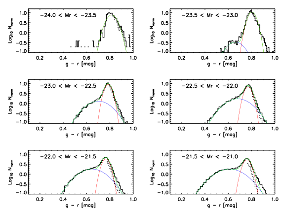
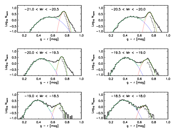
Figure 13: Double-gaussian fits to the bimodal color-magnitude relation provide a good description except in the range $-18.5\leq M_{r}\leq-20.5$ (the “green valley”). Note that, at intermediate/high luminosities, the reddest objects are actually associated with the red tail of the blue component, consistent with the physical expectation that the red sequence may be contaminated by edge-on disks at these luminosities. The dotted line shows the red-end distribution of galaxies (i.e. objects redder than the mean of the red Gaussian component) that also have $b/a>0.6$. Clearly, the reddest objects have smaller $b/a$, consistent with their being edge-on disks.

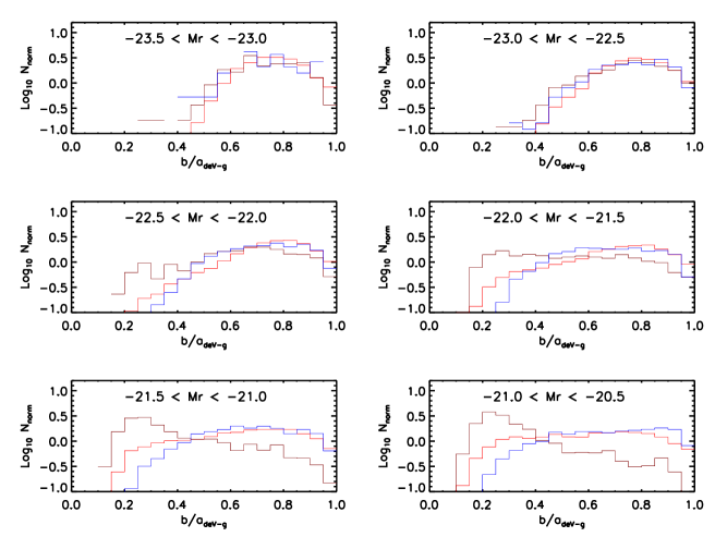
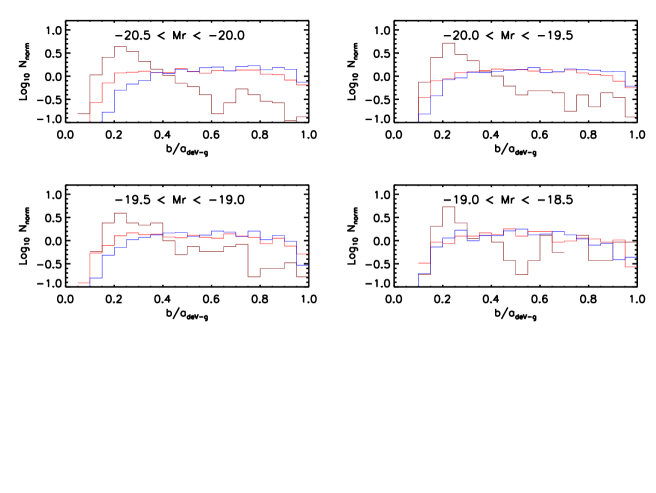
Figure 14: Distribution of axis ratio $b/a$ for objects that are within $0.025$ mags of the peak of the blue component (blue), $0.025$ mags of the peak of the red sequence (red), and 0.1 mags redder than the peak of the red sequence (brown). Compared to the other two populations, this final population has an excess of small $b/a$ values: many objects which are significantly redder than the mean red sequence tend to be edge-on disks.

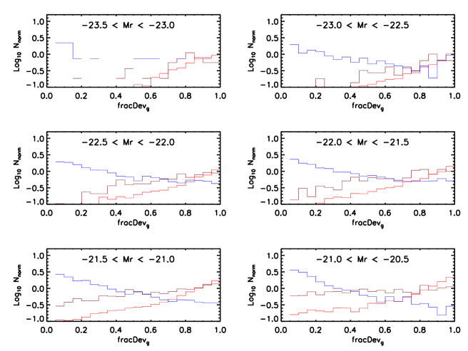
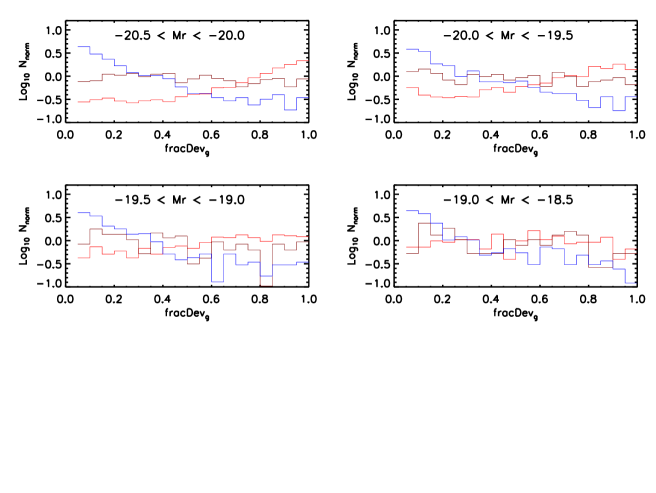
Figure 15: Distribution of fracDev, i.e. the weight of the deVaucouleurs component in the best composite model, for objects that are within $0.025$ mags of the peak of the blue component (blue), $0.025$ mags of the peak of the red sequence (red), and 0.1 mags redder than the peak of the red sequence (brown). Objects near the peak of the blue/red sequence tend to have low/high values of fracDev, as expected. However, objects which lie redward of the red sequence tend to have small values of fracDev more often than do objects which lie at the peak of the red sequence.

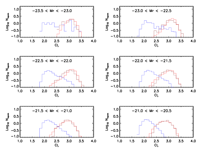
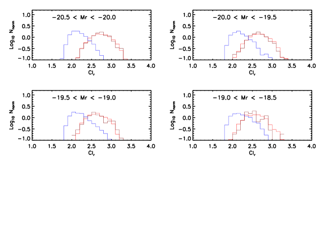
Figure 16: Distribution of the concentration index $C_{r}$ for objects that are within $0.025$ mags of the peak of the blue component (blue), $0.025$ mags of the peak of the red sequence (red), and 0.1 mags redder than the peak of the red sequence (brown). The reddest objects, which the previous figures showed tend to have small $b/a$ and fracDev, have $C_{r}$ values which are indistinguishable from those of genuine red sequence galaxies. Hence, cuts on concentration are not a reliable way to identify and eliminate such objects.

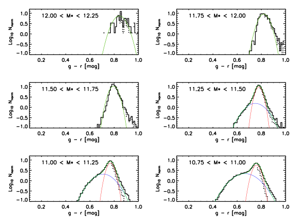
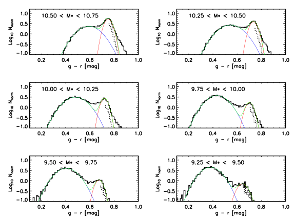
Figure 17: Same format as Figure 13 but showing the double-gaussian fits to the bimodal color-$M_{*}$ relation.

Table 2: Parameters of double-Gaussian fits to the $g-r$ model color distribution in narrow bins in $M_{r}$.

$M_{r}$	$g-r$ (RED)	$rms$ (RED)	$g-r$ (BLUE)	$rms$ (BLUE)	$\%$ (RED)	$\%$ (BLUE)	Ngal
$-23.62$	$0.815$	$0.043$	$0.000$	$0.000$	$1.000$	$0.000$	$517$
$-23.16$	$0.803$	$0.033$	$0.660$	$0.070$	$0.910$	$0.060$	$4413$
$-22.69$	$0.785$	$0.030$	$0.700$	$0.100$	$0.692$	$0.326$	$16906$
$-22.22$	$0.770$	$0.031$	$0.682$	$0.105$	$0.528$	$0.447$	$38080$
$-21.74$	$0.765$	$0.032$	$0.645$	$0.110$	$0.473$	$0.496$	$53391$
$-21.26$	$0.760$	$0.034$	$0.610$	$0.120$	$0.443$	$0.541$	$50603$
$-20.77$	$0.753$	$0.035$	$0.555$	$0.120$	$0.412$	$0.541$	$39172$
$-20.28$	$0.740$	$0.037$	$0.495$	$0.115$	$0.371$	$0.548$	$25833$
$-19.79$	$0.723$	$0.030$	$0.440$	$0.090$	$0.271$	$0.564$	$14081$
$-19.28$	$0.700$	$0.050$	$0.415$	$0.090$	$0.269$	$0.654$	$8114$
$-18.78$	$0.680$	$0.045$	$0.390$	$0.085$	$0.180$	$0.724$	$4817$
$-18.29$	$0.660$	$0.050$	$0.382$	$0.095$	$0.150$	$0.810$	$2892$
$-17.80$	$0.630$	$0.050$	$0.365$	$0.090$	$0.150$	$0.857$	$1506$

Table 3: Parameters of double-Gaussian fits to the $g-r$ model color distribution in narrow bins in $\log_{10}M_{\star}$.

Log${}_{10}M_{*}/M_{\odot}$	$g-r$ (RED)	$rms$ (RED)	$g-r$ (BLUE)	$rms$ (BLUE)	$\%$ (RED)	$\%$ (BLUE)	Ngal
$12.04$	$0.843$	$0.048$	$0.000$	$0.000$	$1.000$	$0.000$	$89$
$11.81$	$0.820$	$0.040$	$0.000$	$0.000$	$0.922$	$0.000$	$1313$
$11.58$	$0.795$	$0.035$	$0.000$	$0.000$	$0.939$	$0.000$	$7943$
$11.35$	$0.780$	$0.028$	$0.750$	$0.080$	$0.688$	$0.311$	$24943$
$11.11$	$0.770$	$0.030$	$0.708$	$0.085$	$0.541$	$0.447$	$48026$
$10.88$	$0.760$	$0.032$	$0.665$	$0.100$	$0.457$	$0.551$	$55556$
$10.63$	$0.751$	$0.032$	$0.590$	$0.090$	$0.425$	$0.530$	$45702$
$10.39$	$0.735$	$0.032$	$0.545$	$0.095$	$0.313$	$0.643$	$31315$
$10.14$	$0.720$	$0.030$	$0.480$	$0.090$	$0.203$	$0.699$	$19064$
$9.89$	$0.702$	$0.032$	$0.433$	$0.085$	$0.136$	$0.788$	$11693$
$9.64$	$0.675$	$0.033$	$0.405$	$0.085$	$0.091$	$0.852$	$7077$
$9.39$	$0.645$	$0.045$	$0.380$	$0.080$	$0.079$	$0.902$	$4388$
$9.15$	$0.610$	$0.045$	$0.355$	$0.080$	$0.062$	$0.882$	$2463$

The distribution of colors at fixed $L_{r}$ is well-known to be bimodal. The smooth curves in Figure 13 show the result of fitting the sum of two gaussian components to the $g-r$ distribution at each $L_{r}$ (e.g. Baldry et al. 2004; Skibba & Sheth 2009). Note that the red sequence is considerably narrower than the bluer component. The parameters of these fits are provided in Table 2, and are used in the main text.

Figure 13 shows that, except in the range $-18.5\leq M_{r}\leq-20.5$ or $9.5\leq\log M_{*}/M_{\odot}\leq 10.25$ the double-gaussian is a good description of the measurements. However, at intermediate $L$ and $M_{*}$, it is unable to describe the transition region between the two populations. (Table 2 shows that, in this regime, the double-Gaussian decomposition only accounts for 90% of the objects.) Since this is fainter than the scales on which we see curvature in the color-magnitude relation, this is not a major concern. However, at slightly larger luminosities, the fits assign the reddest objects to the red tail of the blue component. Is this a limitation of the statistical decomposition, or does it reflect something physical? If it is physical, then this cautions against using sharp cuts in color to isolate early-type galaxies.

The dotted line in Figure 13 shows the red-end distribution of galaxies (i.e. objects redder than the mean of the red Gaussian component) with $b/a>0.6$. This distribution is better fit by the red Gaussian component than by the red tail of the blue component. This shows that the objects which populate the extremely red tail of the blue Gaussian component tend to have small $b/a$.

To address this further, Figures 14–16 show the distribution of axis ratios $b/a$, and two measures of the shape of the light profile, fracDev and concentration index, for objects that lie close to the peak of the blue and red sequences, and that lie 0.1 mags redward of the red sequence. Notice that these reddest objects tend to have small values of $b/a$. This suggests that they are edge-on disks, something which is corroborated by the fact that the distribution of fracDev also extends to smaller values, characteristic of late-type galaxies, than it does for objects on the red sequence. The distribution of concentrations, however, is just like that for objects on the red sequence, but note that there is significant overlap in between the distributions defined by the red and blue sequences.

That the reddest objects at intermediate luminosity are late-type galaxies is also seen in Figure 13 of Bernardi et al. (2010a) which shows how the bimodal color-magnitude distribution is built up by objects of different morphological type. Clearly, the reddest objects at $M_{r}\geq-22.5$ are primarily of type Sa and later – they are not ellipticals. In particular, they are not what one typically associates with the red sequence. That edge-on disks are amongst the reddest objects is not surprising. However, given the wide-spread use of concentration as a way of identifying red-sequence galaxies, our finding that concentration does such a poor job of identifying edge-on disks is disturbing. Our results caution against using sharp cuts in color or concentration for identifying early-type galaxies.

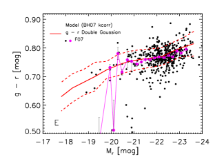
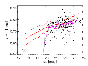
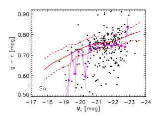
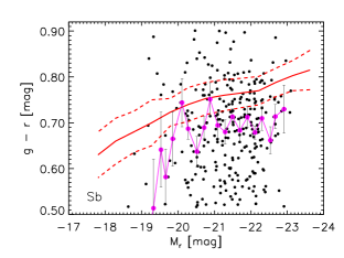
Figure 18: Color-magnitude relation in the Fukugita et al. (2007) sample for types E, S0, Sa, and Sb. Small filled circles show the objects, large filled circles connected by jagged line, show the mean color in bins of $M_{r}$ having width 0.25 mags. Thick solid and associated dashed lines (same in all panels), show the red sequence defined by our double-Gaussian fits to the full SDSS sample (see Table 2). Sas and Sbs dominate the numbers redward of the red sequence.

A.2 Dependence on morphology

One of our goals is to compare measurements on subsamples defined by relatively simple criteria (e.g. concentration index, bimodality) with morphologically selected subsamples. To this end, we use the morphological classification provided by Fukugita et al. (2007). Briefly, Fukugita et al. have provided morphological classifications (Hubble type T) for a subset of 2253 SDSS galaxies brighter than $m_{\tt Pet}=16$ in the $r-$band, selected from 230 deg² of sky. Of these, 1866 have spectroscopic information. Here, we group galaxies classified with half-integer T into the smaller adjoining integer bin (except for the E class; see also Huang & Gu 2009 and Oohama et al. 2009). In the following, we set E (T = 0 and 0.5), S0 (T = 1), Sa (T = 1.5 and 2), Sb (T = 2.5 and 3), and Scd (T = 3.5, 4, 4.5, 5, and 5.5). This gives a fractional morphological mix of (E, S0, Sa, Sb, Scd) = (0.269, 0.235, 0.177, 0.19, 0.098). Note that this is the mix in a magnitude limited catalog – meaning that brighter galaxies (typically earlier-types) are over-represented.

Figure 18 compares the red sequence defined by our double-Gaussian fit to the color-magnitude relations defined by the different morphological types in the (significantly smaller) Fukugita et al. sample. The top left panel shows that ellipticals do indeed lie along the same red sequence defined by the double-Gaussian fits; in particular, the steeper slopes at low and high luminosities, returned by our double-Gaussian fits to the full sample, are also evident in the smaller Fukugita et al. sample (see Huang & Gu 2009 for a more detailed analysis of the “blue” ellipticals with $g-r\leq 0.6$ – they show either a star forming, AGN or post-starburst spectrum). Thus, the curvature is not due to the fact that the mix of morphological types depends on luminosity.

While S0s tend to define the same red sequence, a larger fraction are blue (top right). The central panels show that types Sa and Sb can be both very red and very blue, and even types Sc and Sd can have rather red colors. These red late-type galaxies are edge on disks; whereas any straight color cut will misleadingly group such objects together with early-types, the double-Gaussian decomposition correctly assigns these reddest objects at intermediate and low luminosities to the blue sequence.

Appendix B Systematic effects

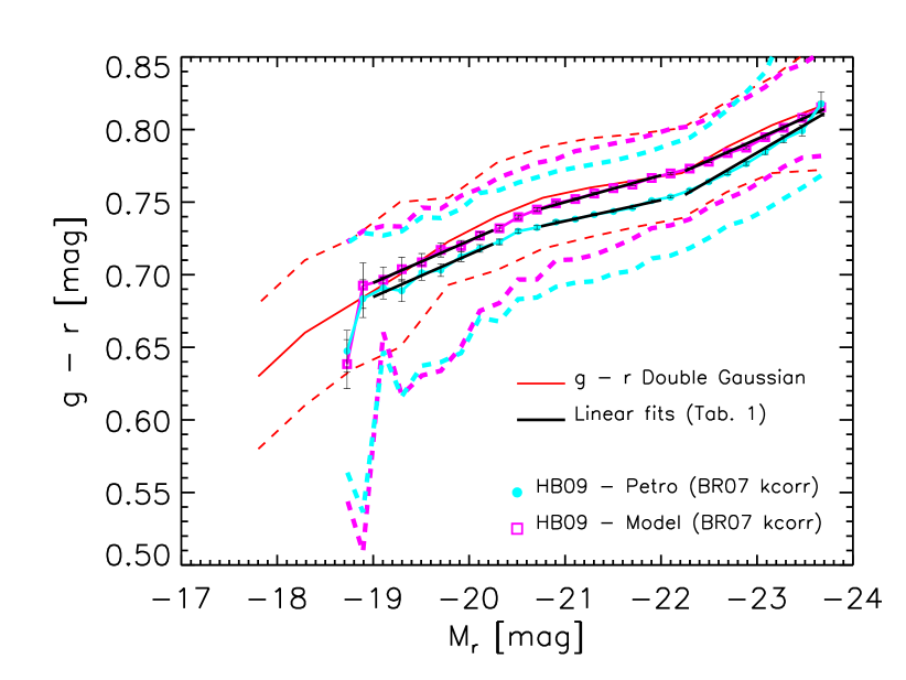
Figure 20: Dependence of color-magnitude relation on the scale on which colors were defined. Model colors, which have higher signal-to-noise ratio, probe smaller scales, so are redder than Petrosian colors. The color offset is largest at $M_{r}\sim-22$, the luminosity scale at which color gradients are maximal (Roche et al. 2010).

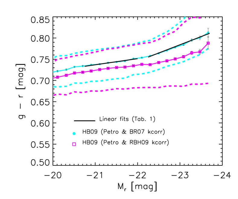
Figure 21: Dependence of color-magnitude relation on the choice of $k$-correction: Blanton & Roweis (2007; BR07) and Roche et al. (2009; RBH09). Spectral-based $k$-corrections (i.e. RBH09) appear to result in bluer colors and less curvature; some of this is simply a consequence of the fact that the spectra are taken using fibers of a fixed aperture.

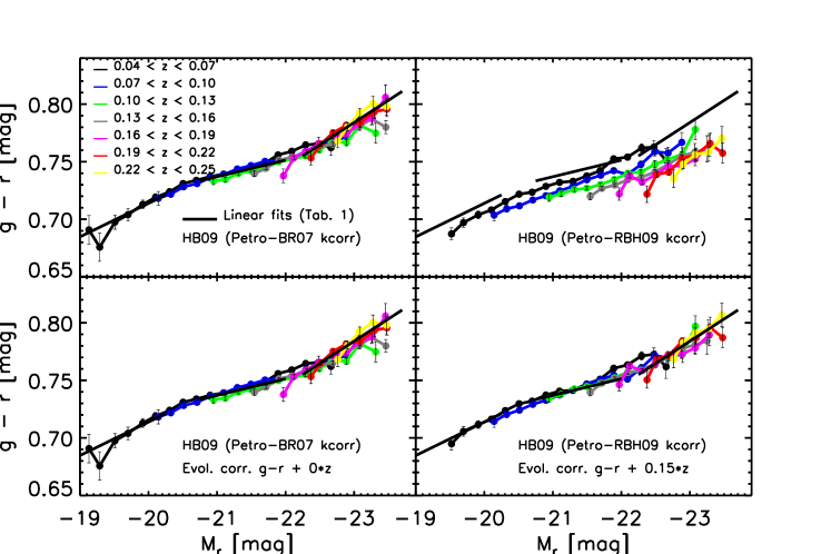
Figure 22: Dependence of color-magnitude relation on the choice of $k$- and evolution corrections: Blanton & Roweis (2007; BR07 – left panels) and Roche et al. (2009; RBH09 – right panels). Different lines (colors) show the color-magnitude relation in different redshift bins as labeled. No evolution correction has been applied in the top panels. Once luminosity evolution has been accounted for (bottom panels) the curvature does not depend on the $k$-correction (note that the evolution correction does depend on the $k$-correction).

B.1 Effects of color gradients

Because the curvature in the red sequence we reported in the main text is small, we have checked if it is robust to changes in how we estimate the colors and luminosities.

The main text showed that the color-magnitude relation shows three distinct regimes (Table 1 reports fits), whether one uses model or Petrosian quantities (compare Figures 1 and 2), despite the fact that Petrosian colors are slightly bluer than model colors. The blueward shift occurs because the model color probes the half-light radius, whereas the Petrosian color is based on a larger physical scale, and early-type galaxies have negative color gradients (i.e., the are redder in the core; e.g. Wu et al. 2005). Although color gradients decrease with $\sigma$, they are a complicated function of luminosity: Gradients are largest for objects with $M_{r}=-22$, and are smaller for brighter or fainter objects (Roche et al. 2010). Figure 20 shows a direct comparison: the difference between the Petrosian and model color-magnitude relations in the Hyde-Bernardi sample is largest at $M_{r}\sim-22$ (note that the $M_{r}$ is the cmodel quantity).

For our purposes here, the main point is that three distinct regimes are seen whatever our choice of color, although it is interesting that they are slightly more obvious using colors which sample more of the total light of the galaxy: at intermediate luminosities, the slope of the color-magnitude relation is flatter by a factor of two for Petrosian rather than model colors. (The scatter around the mean relations is larger for Petrosian quantities, in part because of measurement errors – recall from Section 2.1 that the model magnitudes are better measured.)

B.2 Dependence on $k$- and evolution corrections

We have also tested for systematic effects which arise from $k$- and evolution corrections. Our default has been to use values from Blanton & Roweis (2007), which are based on fitting templates to the observed colors. However, Roche et al. (2009) have recently described the results of estimating $k$-corrections from the spectra themselves. If we do not account for evolution, then the colors from the spectral-based $k$-corrections are slightly bluer at the bright end (Figure 21), resulting in weaker curvature. However, we have yet to account for luminosity evolution. The top panels in Figure 22 show the color-magnitude relation in different redshift bins, before correcting for evolution, for the Blanton & Roweis (left) and Roche et al. (right) $k$-corrections. (The plot uses Petrosian colors, but the discussion is valid for the model colors as well.) It is clear that we measure different evolution in the two cases: the evolution in $g-r$ is negligible when using the Blanton & Roweis $k$-corrections (bottom left), while $g-r$ should be reddened by $0.15z$ for Roche et al. (bottom right). Once the color has been corrected for evolution in this way, the curvatures at the faint and bright ends are similar.

There is an additional subtle effect which arises from the fact that the spectra come from fibers having a fixed angular diameter of 3 arcsecs. Color gradients mean that the restframe light in the fiber from a higher redshift object will be slightly bluer, and this affects the spectral-based $k$-correction of Roche et al. (2009). In a magnitude limited sample, the more luminous objects are seen to higher redshifts, so this aperture effect can make the $k$-corrections masquerade as or erase curvature in the color-magnitude relation. The top right panel of Figure 22 also shows that if we restrict the sample to narrow redshift ranges, thus reducing both the evolution and simplifying aperture effects, the curvature in the color-magnitude diagram is still evident, at least in those bins where we have a sufficiently large range of luminosities. (Of course, the significance of the curvature is smaller, because of the smaller sample sizes.)

This is important because Hao et al. (2009) report that the slope of the color magnitude relation is steeper at $z\sim 0.3$ than at $z\sim 0.1$, and they interpret this as evolution in the slope of the relation. We see this too – the highest redshift samples (which span $M_{r}<-22.5$) appear to define steeper relations than those at $z<0.1$. However, because ours is a magnitude limited sample, these highest redshifts do not probe faint objects. Our lowest and intermediate redshift samples, which include a wider range of luminosities, show a slight upturn from intermediate to high luminosities, even at fixed redshift. Therefore, rather than concluding that the slope is evolving, we conclude that the slope depends on luminosity.

Appendix C Sizes and velocity dispersions in zero-energy mergers

We assume that the final object is in virial equilibrium, that it formed from the merger of two smaller virialized objects in which mass was conserved, and that the total energy of the orbits which led to the merger was zero (sometimes called parabolic orbits).

The virial condition means that $-W=2K$ for all of the objects, meaning that the total energy for each object is $K+W=K-2K=-K=W/2$. If the mergers are of equal mass objects, each of mass $m$, then the total energy of the system before the merger is $-mv^{2}/2-mv^{2}/2=-2m\,(v^{2}/2)$ (because there is no contribution from the orbital energy). However, the final object will have mass $2m$. This with energy conservation and the constraint that the final object is virialized means that $v$ must be unchanged.

If the mergers are not equal mass, then

$$-\frac{mv^{2}}{2}-\frac{MV^{2}}{2} = -\frac{MV^{2}}{2}(f(v/V)^{2}+1)$$

$$= -\frac{G(1+f)^{2}M^{2}}{2R(R_{f}/R)}=-(1+f)\,\frac{MV_{f}^{2}}{2},$$

where the larger object has mass $M$, size $R$ and velocity dispersion $V$, the smaller one has mass $m=fM$ and velocity dispersion $v\leq V$, and $R_{f}$ and $V_{f}$ are the size and velocity dispersion of the final object which has mass $M(1+f)$. Eliminating a factor of $M(1+f)$ from the second and third expressions, and then using the fact that $-GM/2R=V^{2}/2$, gives an expression for $R_{f}/R$ in terms of $f$ and $v/V$:

$$\frac{R_{f}}{R}=\frac{(1+f)^{2}}{1+f(v/V)^{2}}.$$ (4)

In addition, equating the second and final expressions yields

$$\frac{V_{f}^{2}}{V^{2}}=\frac{1+f(v/V)^{2}}{1+f}.$$ (5)

The density of the final object is proportional to

$$\frac{V_{f}^{2}}{R_{f}^{2}}=\frac{V^{2}}{R^{2}}\frac{1+f(v/V)^{2}}{1+f}\frac{[1+f(v/V)^{2}]^{2}}{(1+f)^{4}}.$$ (6)

Since $v/V\leq 1$, the size will increase, and the velocity dispersion and density will both decrease. The limiting case is when $f=1$: then $R_{f}=2R$, $V_{f}=V$ and the density is smaller by a factor of 4. This is the basis for the claim that major mergers double the size without changing the velocity dispersion. (Doubling the size decreases the density by a factor of 4 rather than $2^{3}=8$, because the mass has increased by a factor of 2.) When $f\ll 1$ then $R_{f}/R\to 1+2f$ whereas $V_{f}/V\to 1-f/2$: for minor mergers, the fractional change to the size is larger than that to the velocity dispersion. The fractional change in density due to a minor merger is even larger: it scales as $-5f$.

References

- [] Baldry, I. K., Glazebrook, K., Brinkmann, J., Ivezic, Z., Lupton, R. H., Nichol, R. C. & Szalay, A. S. 2004, ApJ, 600, 681
- [Bell et al.(2003)] Bell E. F., McIntosh D. H., Katz N., & Weinberg M. D., 2003, ApJS, 149, 289
- [Bernardi et al. 2003a] Bernardi M., et al. 2003a, AJ, 125, 1817
- [Bernardi et al. 2003b] Bernardi M., et al. 2003b, AJ, 125, 1866
- [Bernardi et al. 2003c] Bernardi M., et al. 2003c, AJ, 125, 1882
- [Bernardi et al. 2005] Bernardi M., Sheth R. K., Nichol R. C., Schneider D. P., Brinkmann J., 2005, AJ, 129, 61
- [Bernardi et al.(2006)] Bernardi, M., Nichol, R. C., Sheth, R. K., Miller, C. J., & Brinkmann, J. 2006, AJ, 131, 1288
- [Bernardi et al. 2007] Bernardi, M., Hyde, J. B., Sheth, R. K., Miller, C. J., & Nichol, R. C. 2007, AJ, 133, 1741
- [Bernardi et al. 2008] Bernardi, M., Hyde, J. B., Fritz, A., Sheth, R. K., Gebhardt, K. & Nichol, R. C. 2008, MNRAS, 391, 1191
- [Bernardi 2009] Bernardi, M. 2009, MNRAS, 395, 1491
- [Bernardi et al. 2010a] Bernardi M., Shankar, F., Hyde, J. B., Mei, S., Marulli, F. & Sheth, R. K. 2010a, MNRAS, 404, 2087
- [Bernardi et al. 2010b] Bernardi M., Roche, N., Shankar, F. & Sheth, R. K. 2010b, MNRAS, submitted
- [] Blanton, M. R., Eisenstein, D., Hogg, D. W., Schlegel, D. J. & Brinkmann, J. 2005, ApJ, 629, 143
- [Blanton & Roweis (2007)] Blanton M. R., Roweis S., 2007, AJ, 133, 734
- [Blanton & Berlind 2007] Blanton M. R., Berlind A. A., 2007, ApJ, 664, 791
- [] Baldry, I. K., Glazebrook, K., Brinkmann, J., Ivezic, Z., Lupton, R. H., Nichol, R. C. & Szalay A. S. 2004, ApJ, 600, 681
- [] Bower, R. G., Lucey, J. R. & Ellis, R. S. 1992, MNRAS, 254, 601
- [] Brown, M. J. I., Dey, A., Jannuzi, B. T., Brand, K., Benson, A. J., Brodwin, M., Croton, D. J., & Eisenhardt, P. R. 2007, ApJ, 654, 858
- [] Cool, R. J., et al. 2008, ApJ, 682, 919
- [] Eliche-Moral, M. C., Prieto, M., Gallego, J. & Zamorano, J. 2010, ApJ, submitted (arXiv:1003.0686)
- [] Faber, S. M. et al. 2007, ApJ, 665, 265
- [Fukugita et al.(2007)] Fukugita M., et al., 2007, AJ, 134, 579
- [] Gallazzi, A., Charlot, S., Brinchmann, J., White, S. D. M. & Tremonti, C. 2005, MNRAS, 362, 41
- [] Gallazzi, A., Charlot, S., Brinchmann, J. & White, S. D. M. 2006, MNRAS, 370, 1106
- [] Graham A.W., 2008, ApJ, 680, 143
- [] Guo, Q. & White, S. D. M. 2008, MNRAS, 384, 2
- [] Hao, J. et al. 2009, ApJ, 702, 745
- [Hyde & Bernardi(2009)] Hyde J. B. & Bernardi M., 2009, MNRAS, 394, 1978
- [Hopkins et al.(2010)] Hopkins, P. F., et al. 2010, ApJ, in press (arXiv:0906.5357)
- [Huang & Gu(2009)] Huang S., Gu, Q.-S., 2009, MNRAS, 398, 1651
- [] Mo H. J., White, S. D. M., 1996, MNRAS, 282, 347
- [] Kauffmann, G., et al. 2003, MNRAS, 341, 33
- [] Kodama, T., Arimoto, N., Barger, A. J. & Aragón-Salamanca, A. 1998, A&A, 334, 99
- [Lintott et al.(2008)] Lintott C., et al., 2008, MNRAS, 389, 1179
- [] Matsuoka, Y. & Kawara, K. 2010, MNRAS, in press (arXiv:1002.0471)
- [Mei et al.(2009)] Mei, S., et al. 2009, ApJ, 690, 42
- [] Mitchell, J. L., Keeton, C. R., Frieman, J. A. & Sheth, R. K. 2005, ApJ, 622, 81
- [Nakamura et al.(2003)] Nakamura O., Fukugita M., Yasuda N., Loveday J., Brinkmann J., Schneider D. P., Shimasaku K., SubbaRao M., 2003, AJ, 125, 1682
- [Oohama et al.(2009)] Oohama, N., Okamura, S., Fukugita, M., Yasuda, N. & Nakamura, O., 2009, ApJ, 705, 245
- [] Peng, Y. et al. 2010, ApJ, submitted (arXiv:1003.4747)
- [] Pipino, A. & Matteucci, F. 2008, A&A, 486, 763
- [] Robaina, A. R. et al. 2010, ApJ, 719, 844
- [] Roche, N., Bernardi, M. & Hyde, J. B. 2009, MNRAS, 398, 1549
- [] Roche, N., Bernardi, M. & Hyde, J. B. 2010, MNRAS, 407, 1231
- [] Sandage, A. & Visvanathan, N. 1978, 223, 707
- [] Shankar, F. & Bernardi, M., 2009, MNRAS, 396, L76
- [] Shankar, F., Marulli, F., Bernardi, M., Dai, X., Hyde, J. B. & Sheth, R. K. 2010a, MNRAS, in press (arXiv0912.0012)
- [] Shankar, F., Marulli, F., Bernardi, M., Boylan-Kolchin, M., Dai, X. & Khochfar, S., 2010b, MNRAS, in press (arXiv:1002.3394)
- [] Shen, S., Mo, H. J., White, S. D. M., Blanton, M. R., Kauffmann, G., Voges, W., Brinkmann, J. & Csabai, I. 2003, MNRAS, 343, 978
- [] Sheth, R. K., 1998, MNRAS, 300, 1057
- [] Sheth, R. K., Jimenez, R., Panter, B., Heavens, A. F., 2006, ApJL, 650, L25
- [] Skelton, R. E., Bell, E. F. & Somerville, R. S. 2009, ApJL, 699, 9
- [] Skibba, R. A. & Sheth, R. K. 2009, MNRAS, 392, 1080
- [] Strateva, I., et al. 2001, AJ, 122, 1861
- [] Trager, S. C., Faber, S. M., Worthey, G., & González, J. J. 2000, AJ, 120, 165
- [Wake et al. 2008] Wake D., et al., 2008, MNRAS, 387, 1045
- [] Willmer, C. N. A, et al. 2006, ApJ, 647, 853
- [] Wu, H., Shao, Z., Mo, H. J., Xia, X. & Deng, Z. 2005, ApJ, 622, 244
- [] Zehavi, I. et al. 2005, 630, 1