Fast and slow two-fluid magnetic reconnection

Abstract

We present a two-fluid magnetohydrodynamics (MHD) model of quasi-stationary, two-dimensional magnetic reconnection in an incompressible plasma composed of electrons and ions. We find two distinct regimes of slow and fast reconnection. The presence of these two regimes can provide a possible explanation for the initial slow build up and subsequent rapid release of magnetic energy frequently observed in cosmic and laboratory plasmas.

1 Introduction

Magnetic reconnection is the physical process by means of which magnetic field lines join one another and rearrange their topology. Magnetic reconnection is believed to be the mechanism by which magnetic energy is converted into kinetic and thermal energy in the solar atmosphere, the Earth’s magnetosphere, and in laboratory plasmas [1, 2, 3, 4, 5, 6, 7]. Many reconnection related physical phenomena observed in cosmic and laboratory plasmas exhibit a two-stage behavior. During the first stage, magnetic energy is slowly built up and stored in the system with relatively little reconnection occurring. The second stage is characterized by a sudden and rapid release of the accumulated magnetic energy due to a fast reconnection process. For example, a solar flare is powered by a sudden (on timescale ranging from minutes to tens of minutes) release of magnetic energy stored in the upper solar atmosphere [4]. Because the value of the Spitzer electrical resistivity is very low in hot plasmas, magnetic energy release rates predicted by a simple single-fluid MHD description of magnetic reconnection are much slower than the rates observed during fast reconnection events in astrophysical and laboratory plasmas [1, 3, 4, 5, 6, 7]. One of the most promising solutions of this discrepancy is the two-fluid MHD theoretical approach to magnetic reconnection [1, 4, 5, 6, 7, and references therein]. Recently a model of two fluid reconnection in a electron-proton plasma was presented in [8]. In this paper, we consider a more general case of two-fluid reconnection in electron-ion and electron-positron plasmas, and we present derivations in detail. In the discussion section, we also argue that the slow and fast reconnection regimes predicted by our model, can provide a possible explanation for the observed two-stage reconnection behavior.

2 Two-fluid MHD equations

In this study, we use physical units in which the speed of light $c$ and four times $\pi$ are replaced by unity, $c=1$ and $4\pi=1$. To rewrite our equations in the Gaussian centimeter-gram-second (CGS) units, one needs to make the following substitutions: magnetic field ${\bf B}\rightarrow{\bf B}/\sqrt{4\pi}$, electric field ${\bf E}\rightarrow c{\bf E}/\sqrt{4\pi}$, electric current ${\bf j}\rightarrow\sqrt{4\pi}\,{\bf j}/c$, electrical resistivity $\eta\rightarrow\eta c^{2}/4\pi$, the proton electric charge $e\rightarrow\sqrt{4\pi}\,e/c$.

We consider an incompressible two-component plasma, composed of electrons and ions. We assume the plasma is non-relativistic and, therefore, quasi-neutral. The ions are assumed to have mass $m_{i}$ and electric charge $Ze$, while the electrons have mass $m_{e}$ and charge $-e$. Because of incompressibility, the electron and ion number densities are constant,

$$n_{e}\equiv n={\rm const},\qquad n_{i}=Z^{-1}n={\rm const},$$ (1)

where the last formula follows from the plasma quasi-neutrality condition $Zen_{i}=en_{e}$. The plasma density $\rho$, the electric current ${\bf j}$ and the plasma (center-of-mass) velocity ${\bf V}$ are

$$\rho = m_{i}n_{i}+m_{e}n_{e}=n(Z^{-1}m_{i}+m_{e})={\rm const},$$ (2)

$${\bf j} = Zen_{i}{\bf u}^{i}-en_{e}{\bf u}^{e}=ne({\bf u}^{i}-{\bf u}^{e}),$$ (3)

$${\bf V} = (m_{i}n_{i}{\bf u}^{i}+m_{e}n_{e}{\bf u}^{e})/\rho=n(Z^{-1}m_{i}{\bf u}^{i}+m_{e}{\bf u}^{e})/\rho.$$ (4)

Here ${\bf u}^{e}$ and ${\bf u}^{i}$ are the mean electron and ion velocities, which can be found from the above equations,

$${\bf u}^{e}={\bf V}-(m_{i}/Ze\rho){\bf j},\qquad{\bf u}^{i}={\bf V}+(m_{e}/e\rho){\bf j}.$$ (5)

The equations of motion for the electrons and ions are [9, 10]

$$n_{e}m_{e}\left[\partial_{t}{\bf u}^{e}+({\bf u}^{e}{\bf\nabla}){\bf u}^{e}\right] = -{\bf\nabla}P_{e}-n_{e}e({\bf E}+{\bf u}^{e}\times{\bf B})-{\bf K},$$ (6)

$$n_{i}m_{i}\left[\partial_{t}{\bf u}^{i}+({\bf u}^{i}{\bf\nabla}){\bf u}^{i}\right] = -{\bf\nabla}P_{i}+n_{i}Ze({\bf E}+{\bf u}^{i}\times{\bf B})+{\bf K},$$ (7)

where $P_{e}$ and $P_{i}$ are the electron and ion pressure tensors, and ${\bf K}$ is the resistive frictional force due to electron-ion collisions. Force ${\bf K}$ can be approximated as [9, 10]

$${\bf K}=n^{2}e^{2}\eta({\bf u}^{e}-{\bf u}^{i})=-ne\eta{\bf j},$$ (8)

where $\eta$ is the electrical resistivity, and we use equation (3). For simplicity, we assume isotropic resistivity, and we also neglect ion-ion and electron-electron collisions and the corresponding viscous forces. Substituting equations (1), (5) and (8) into equations (6) and (7), we obtain

$$nm_{e}\left[\partial_{t}{\bf V}+({\bf V}{\bf\nabla}){\bf V}\right]$$

$$\qquad-(nm_{e}m_{i}/Ze\rho)\left[\partial_{t}{\bf j}+({\bf V}{\bf\nabla}){\bf j}+({\bf j}{\bf\nabla}){\bf V}-(m_{i}/Ze\rho)({\bf j}{\bf\nabla}){\bf j}\right]$$

$$\;\;{}=-{\bf\nabla}P_{e}-ne{\bf E}-ne{\bf V}\times{\bf B}+(m_{i}n/Z\rho){\bf j}\times{\bf B}+ne\eta{\bf j},$$ (9)

$$Z^{-1}nm_{i}\left[\partial_{t}{\bf V}+({\bf V}{\bf\nabla}){\bf V}\right]$$

$$\qquad+(nm_{e}m_{i}/Ze\rho)\left[\partial_{t}{\bf j}+({\bf V}{\bf\nabla}){\bf j}+({\bf j}{\bf\nabla}){\bf V}+(m_{e}/e\rho)({\bf j}{\bf\nabla}){\bf j}\right]$$

$$\;\;{}=-{\bf\nabla}P_{i}+ne{\bf E}+ne{\bf V}\times{\bf B}+(m_{e}n/\rho){\bf j}\times{\bf B}-ne\eta{\bf j}.$$ (10)

We sum equations (9) and (10) together and obtain the plasma momentum equation

$$\rho\left[\partial_{t}{\bf V}+({\bf V}{\bf\nabla}){\bf V}\right]+(m_{e}m_{i}/Ze^{2}\rho)({\bf j}{\bf\nabla}){\bf j}=-{\bf\nabla}P+{\bf j}\times{\bf B},$$ (11)

where $P=P_{e}+P_{i}$ is the total pressure. Next we subtract equation (10) multiplied by $Zm_{e}/m_{i}$ from equation (9) and obtain the generalized Ohm’s law

$${\bf E} = \eta{\bf j}-{\bf V}\times{\bf B}+(m_{i}/Ze\rho)(1-Zm_{e}/m_{i}){\bf j}\times{\bf B}$$ (12)

$$-(m_{i}/Ze\rho)[{\bf\nabla}P_{e}-(Zm_{e}/m_{i}){\bf\nabla}P_{i}]$$

$$+(m_{e}m_{i}/Ze^{2}\rho)\left[\partial_{t}{\bf j}+({\bf V}{\bf\nabla}){\bf j}+({\bf j}{\bf\nabla}){\bf V}\right.$$

$$\qquad\qquad\left.-(m_{i}/Ze\rho)(1-Zm_{e}/m_{i})({\bf j}{\bf\nabla}){\bf j}\right].$$

It is convenient to introduce the ion and electron inertial lengths

$$\begin{array}[]{l}d_{i}\equiv(m_{i}/n_{i}Z^{2}e^{2})^{1/2}=(m_{i}/Zne^{2})^{1/2},\\ d_{e}\equiv(m_{e}/n_{e}e^{2})^{1/2}=(m_{e}/ne^{2})^{1/2}\leq d_{i},\end{array}$$ (15)

and constants

$$\begin{array}[]{l}\omega_{+}^{2}\equiv(1+Zm_{e}/m_{i})^{-1}=(1+d_{e}^{2}/d_{i}^{2})^{-1},\\ \omega_{-}^{2}\equiv 1-Zm_{e}/m_{i}=1-d_{e}^{2}/d_{i}^{2}\geq 0.\end{array}$$ (18)

Here we consider a physically relevant case of $Zm_{e}\leq m_{i}$, so that $d_{e}\leq d_{i}$, $0\leq\omega_{-}^{2}<1$ and $1/2\leq\omega_{+}^{2}<1$. Note that $\omega_{+}^{2}\approx\omega_{-}^{2}\approx 1$ in the case of electron-ion plasma ($Zm_{e}\ll m_{i}$), and $\omega_{+}^{2}=1/2$ and $\omega_{-}^{2}=0$ in the case of electron-positron plasma ($Z=1$ and $m_{i}=m_{e}$).

Using definitions (15) and (18), we obtain for the plasma density (2) expression

$$\rho=m_{i}n/Z\omega_{+}^{2}=n^{2}e^{2}d_{i}^{2}/\omega_{+}^{2},$$ (19)

and we rewrite the plasma momentum equation (11) and Ohm’s law (12) as

$$\rho\left[\partial_{t}{\bf V}+({\bf V}{\bf\nabla}){\bf V}\right]+\omega_{+}^{2}d_{e}^{2}({\bf j}{\bf\nabla}){\bf j}=-{\bf\nabla}P+{\bf j}\times{\bf B},$$ (20)

$${\bf E}=\eta{\bf j}-{\bf V}\!\times\!{\bf B}+(\omega_{+}^{2}\omega_{-}^{2}/ne)\,{\bf j}\!\times\!{\bf B}$$

$$\hphantom{{\bf E}=}-(\omega_{+}^{2}/ne)[{\bf\nabla}P_{e}-(d_{e}^{2}/d_{i}^{2}){\bf\nabla}P_{i}]$$

$$\hphantom{{\bf E}=}+\omega_{+}^{2}d_{e}^{2}\left[\partial_{t}{\bf j}+({\bf V}{\bf\nabla}){\bf j}+({\bf j}{\bf\nabla}){\bf V}-(\omega_{+}^{2}\omega_{-}^{2}/ne)({\bf j}{\bf\nabla}){\bf j}\right]\!.$$ (21)

It is noteworthy that the electron inertia terms, proportional to $d_{e}^{2}$, enter both Ohm’s law and the momentum equation. Although these terms are important for fast two-fluid reconnection (as we shall see below), they have been frequently neglected in the momentum equation in the past . In addition, we note that ${\bf\nabla}\cdot{\bf B}=0$, and also ${\bf\nabla}\cdot{\bf V}=0$ and ${\bf\nabla}\cdot{\bf j}=0$ for incompressible and non-relativistic plasmas.

For convenience of the presentation, below we will refer to the plasma as being electron-ion, even though, unless otherwise stated, our derivations in the next two sections are valid for reconnection in an electron-positron plasma as well.

3 Reconnection layer

We consider two-fluid magnetic reconnection in the classical two-dimensional Sweet-Parker-Petschek geometry, which is shown in figure 1. The reconnection layer is in the $x$-$y$ plane with the $x$- and $y$-axes perpendicular to and along the reconnection layer respectively. The $z$ derivatives of all physical quantities are zero.

The approximate thickness of the reconnection current layer is $2\delta$, which is defined in terms of the out-of-plane current ($j_{z}$) profile across the layer . The approximate length of the out-of-plane current ($j_{z}$) profile along the layer is defined as $2L$. Outside the reconnection current layer the electric currents are weak, the electron inertia is negligible, Ohm’s law (21) reduces to ${\bf E}=-{\bf V}\times{\bf B}+{\bf j}\times{\bf B}/ne=-{\bf u^{e}}\times{\bf B}$ (in the case of electron-ion plasma, $\omega_{+}^{2}\approx\omega_{-}^{2}\approx 1$), and, therefore, the magnetic field lines are frozen into the electron fluid. Thus, $2\delta$ and $2L$ are also approximately the thickness and the length of the electron layer, where electron inertia is important and the electrons are decoupled from the field lines. The ion layer, where the ions are decoupled from the field lines, is assumed to have thickness $2\Delta$ and length $2L_{ext}$, which can be much larger than $2\delta$ and $2L$ respectively. The values of the reconnecting field in the upstream regions outside the electron layer (at $x\approx\delta$) and outside the ion layer (at $x\approx\Delta$) are about the same, $B_{y}\approx B_{ext}$ up to a factor of order unity. This result follows directly from the definition of $2\delta$, and from the $z$-component of the Ampere’s law, $B_{y}(x,y=0)=\int_{0}^{x}j_{z}(x^{\prime},y=0)dx^{\prime}$. The out-of-plane field $B_{z}$ is assumed to have a quadrupole structure (see figure 1) [5, 6, 7] .

The reconnection layer is assumed to have a point symmetry with respect to its geometric center $O$ (see figure 1) and reflection symmetries with respect to the $x$- and $y$-axes. Thus, the $x$-, $y$- and $z$-components of ${\bf V}$, ${\bf B}$ and ${\bf j}$ have the following symmetries: $V_{x}(\pm x,\mp y)=\pm V_{x}(x,y)$, $V_{y}(\pm x,\mp y)=\mp V_{y}(x,y)$, $V_{z}(\pm x,\mp y)=V_{z}(x,y)$, $B_{x}(\pm x,\mp y)=\mp B_{x}(x,y)$, $B_{y}(\pm x,\mp y)=\pm B_{y}(x,y)$, $B_{z}(\pm x,\mp y)=-B_{z}(x,y)$, $j_{x}(\pm x,\mp y)=\pm j_{x}(x,y)$, $j_{y}(\pm x,\mp y)=\mp j_{y}(x,y)$ and $j_{z}(\pm x,\mp y)=j_{z}(x,y)$. The derivations below extensively exploit these symmetries and are similar to the derivations in [8, 11, 12].

We make the following assumptions for the reconnection process. First, resistivity $\eta$ is assumed to be constant and very small, so that the characteristic Lundquist number $S$ is very large,

$$S\equiv V_{A}L_{ext}/\eta\gg 1,\qquad V_{A}\equiv B_{ext}/\sqrt{\rho}.$$ (22)

Here $V_{A}$ is the Alfven velocity. Second, the reconnection process is assumed to be quasi-stationary (or stationary), so that we can neglect time derivatives in the equations above and in the derivations below. This assumption is satisfied if there are no plasma instabilities in the reconnection layer, and the reconnection rate is slow sub-Alfvenic, $E_{z}\ll V_{A}B_{ext}$. Third, we assume that the reconnection layer is thin, $\delta\ll L$ and $\Delta\ll L_{ext}$, which is an assumption related to the previous one. Fourth, we assume that the electron and ion pressure tensors $P_{e}$ and $P_{i}$ are isotropic, therefore, the pressure terms in equations (21) and (20) are assumed to be scalars.

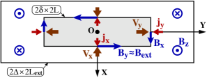
Figure 1: Two-dimensional reconnection layer.

4 Two-fluid reconnection equations

We use Ampere’s law and neglect the displacement current in a non-relativistic plasma to find the components of the electric current

$$j_{x}=\partial_{y}B_{z},\quad j_{y}=-\partial_{x}B_{z},\quad j_{z}=\partial_{x}B_{y}-\partial_{y}B_{x}.$$ (23)

The $z$-component of the current at the central point $O$ (see figure 1) is

$$j_{o}\equiv(j_{z})_{o}=(\partial_{x}B_{y}-\partial_{y}B_{x})_{o}\approx(\partial_{x}B_{y})_{o}\approx B_{ext}/\delta,$$ (24)

where we use the estimates $(\partial_{y}B_{x})_{o}\ll(\partial_{x}B_{y})_{o}$ and $(\partial_{x}B_{y})_{o}\approx B_{ext}/\delta$ at the point $O$. The last estimate follows directly from the definition of $\delta$ as being the half-thickness of the out-of-plane current profile across the reconnection layer.

In the case of a quasi-stationary two-dimensional reconnection, we neglect time derivatives, and Faraday’s law ${{\bf\nabla}\times{\bf E}}=-\partial_{t}{\bf B}$ for the $x$- and $y$-components of the magnetic field results in equations $\partial_{y}E_{z}=-\partial_{t}B_{x}=0$ and $\partial_{x}E_{z}=\partial_{t}B_{y}=0$. Therefore, $E_{z}$ is constant in space, and from the z-component of the generalized Ohm’s law (21) we obtain

$$E_{z} = \eta j_{z}-V_{x}B_{y}+V_{y}B_{x}+(\omega_{+}^{2}\omega_{-}^{2}/ne)(j_{x}B_{y}-j_{y}B_{x})$$ (25)

$$+ \omega_{+}^{2}d_{e}^{2}\left[V_{x}\partial_{x}j_{z}+V_{y}\partial_{y}j_{z}+j_{x}\partial_{x}V_{z}+j_{y}\partial_{y}V_{z}\right.$$

$$\quad\;\left.-(\omega_{+}^{2}\omega_{-}^{2}/ne)(j_{x}\partial_{x}j_{z}+j_{y}\partial_{y}j_{z})\right]=\mbox{constant}.\quad$$

The reconnection rate is determined by the value of $E_{z}$ at the central point $O$, that is

$$E_{z}=\eta j_{o}.$$ (26)

We see that the electric field is balanced only by the resistive term $\eta j_{o}$ at the central point $O$; this is because we assume isotropic pressure tensors in this study. To estimate $j_{o}$, in what follows we neglect time derivatives for a quasi-stationary reconnection and we use the symmetries of the reconnection layer.

The z-component of the momentum equation (20) is

$$\rho(V_{x}\partial_{x}V_{z}+V_{y}\partial_{y}V_{z})+\omega_{+}^{2}d_{e}^{2}(j_{x}\partial_{x}j_{z}+j_{y}\partial_{y}j_{z})=j_{x}B_{y}-j_{y}B_{x}.$$

Taking the second derivatives of this equation with respect to $x$ and $y$ at the point $O$, we obtain

$$\rho(\partial_{x}V_{x})_{o}(\partial_{xx}V_{z})_{o}+\omega_{+}^{2}d_{e}^{2}(\partial_{x}j_{x})_{o}(\partial_{xx}j_{z})_{o}=(\partial_{x}j_{x})_{o}(\partial_{x}B_{y})_{o},$$

$$\rho(\partial_{y}V_{y})_{o}(\partial_{yy}V_{z})_{o}+\omega_{+}^{2}d_{e}^{2}(\partial_{y}j_{y})_{o}(\partial_{yy}j_{z})_{o}=-(\partial_{y}j_{y})_{o}(\partial_{y}B_{x})_{o}.$$

Therefore,

$$\begin{array}[]{l}(\partial_{xx}V_{z})_{o}=-(\partial_{xy}B_{z})_{o}[(\partial_{x}B_{y})_{o}-\omega_{+}^{2}d_{e}^{2}(\partial_{xx}j_{z})_{o}]/\rho(\partial_{y}V_{y})_{o},\\ (\partial_{yy}V_{z})_{o}=(\partial_{xy}B_{z})_{o}[(\partial_{y}B_{x})_{o}+\omega_{+}^{2}d_{e}^{2}(\partial_{yy}j_{z})_{o}]/\rho(\partial_{y}V_{y})_{o},\end{array}$$ (29)

where we use equations (23) and the plasma incompressibility relation $\partial_{x}V_{x}=-\partial_{y}V_{y}$.

Next, we calculate the second derivatives of equation (25) with respect to $x$ and $y$ at the central point $O$ and obtain

$$0 \!=\! \eta(\partial_{xx}j_{z})_{o}-2[(\partial_{x}V_{x})_{o}-(\omega_{+}^{2}\omega_{-}^{2}/ne)(\partial_{x}j_{x})_{o}](\partial_{x}B_{y})_{o}$$

$$+2\omega_{+}^{2}d_{e}^{2}[(\partial_{x}V_{x})_{o}(\partial_{xx}j_{z})_{o}+(\partial_{x}j_{x})_{o}(\partial_{xx}V_{z})_{o}$$

$$\hphantom{{}+2\omega_{+}^{2}d_{e}^{2}[{}}-(\omega_{+}^{2}\omega_{-}^{2}/ne)(\partial_{x}j_{x})_{o}(\partial_{xx}j_{z})_{o}],$$

$$0 \!=\! \eta(\partial_{yy}j_{z})_{o}+2[(\partial_{y}V_{y})_{o}-(\omega_{+}^{2}\omega_{-}^{2}/ne)(\partial_{y}j_{y})_{o}](\partial_{y}B_{x})_{o}$$

$$+2\omega_{+}^{2}d_{e}^{2}[(\partial_{y}V_{y})_{o}(\partial_{yy}j_{z})_{o}+(\partial_{y}j_{y})_{o}(\partial_{yy}V_{z})_{o}$$

$$\hphantom{{}+2\omega_{+}^{2}d_{e}^{2}[{}}-(\omega_{+}^{2}\omega_{-}^{2}/ne)(\partial_{y}j_{y})_{o}(\partial_{yy}j_{z})_{o}].$$

Substituting expressions (29) into these equations and using equations (19), (23) and $\partial_{x}V_{x}=-\partial_{y}V_{y}$, we obtain

$$-\eta(\partial_{xx}j_{z})_{o} = 2(\partial_{y}V_{y})_{o}[(\partial_{x}B_{y})_{o}-\omega_{+}^{2}d_{e}^{2}(\partial_{xx}j_{z})_{o}]$$ (30)

$$\times\big{[}1+{\tilde{\gamma}}(\omega_{-}^{2}-d_{e}^{2}{\tilde{\gamma}}/d_{i}^{2})\big{]},$$

$$-\eta(\partial_{yy}j_{z})_{o} = 2(\partial_{y}V_{y})_{o}[(\partial_{y}B_{x})_{o}+\omega_{+}^{2}d_{e}^{2}(\partial_{yy}j_{z})_{o}]$$ (31)

$$\times\big{[}1+{\tilde{\gamma}}(\omega_{-}^{2}-d_{e}^{2}{\tilde{\gamma}}/d_{i}^{2})\big{]},$$

where we introduce a useful dimensional parameter

$${\tilde{\gamma}}\equiv\omega_{+}^{2}(\partial_{xy}B_{z})_{o}\left/ne(\partial_{y}V_{y})_{o}\right..$$ (32)

In the case of electron-ion plasma ($Zm_{e}\ll m_{i}$ and $\omega_{+}^{2}\approx\omega_{-}^{2}\approx 1$), parameter ${\tilde{\gamma}}$ measures the relative strength of the Hall term $({\bf j}\times{\bf B})_{z}/ne$ and the ideal MHD term $({\bf V}\times{\bf B})_{z}$ inside the electron layer.

Taking the ratio of equations (30) and (31), we obtain

$$(\partial_{y}B_{x})_{o} = (\partial_{x}B_{y})_{o}(\partial_{yy}j_{z})_{o}/(\partial_{xx}j_{z})_{o}-2\omega_{+}^{2}d_{e}^{2}(\partial_{yy}j_{z})_{o}$$ (33)

$$\approx (B_{ext}\delta/L^{2})(1+2\omega_{+}^{2}d_{e}^{2}/\delta^{2}),$$

where we use the estimates $(\partial_{xx}j_{z})_{o}\approx-j_{o}/\delta^{2}$ and $(\partial_{yy}j_{z})_{o}\approx-j_{o}/L^{2}$, and equation (24).

In equation (25), the electric field $E_{z}$ is balanced by the ideal MHD and Hall terms outside the electron layer, where the resistivity and electron inertia terms are insignificant. Therefore,

$$E_{z} \approx -V_{x}B_{y}[1-(\omega_{+}^{2}\omega_{-}^{2}/ne)j_{x}/V_{x}]$$ (34)

$$\approx (\partial_{y}V_{y})_{o}\delta\,B_{ext}(1+\omega_{-}^{2}{\tilde{\gamma}}),$$

$$E_{z} \approx V_{y}B_{x}[1-(\omega_{+}^{2}\omega_{-}^{2}/ne)j_{y}/V_{y}]$$ (35)

$$\approx (\partial_{y}V_{y})_{o}(\partial_{y}B_{x})_{o}L^{2}(1+\omega_{-}^{2}{\tilde{\gamma}})\qquad$$

at the points $(x\approx\delta,y=0)$ and $(x=0,y\approx L)$ respectively. Here we use the estimates $j_{x}\approx(\partial_{xy}B_{z})_{o}\delta$, $j_{y}\approx-(\partial_{xy}B_{z})_{o}L$, $V_{x}\approx-(\partial_{y}V_{y})_{o}\delta$, $V_{y}\approx(\partial_{y}V_{y})_{o}L$, $B_{x}\approx(\partial_{y}B_{x})_{o}L$ and $B_{y}\approx B_{ext}$, and equation (32). The ratio of equations (34) and (35) gives

$$(\partial_{y}B_{x})_{o}\approx B_{ext}\delta/L^{2}\approx B_{ext}^{2}/j_{o}L^{2},$$ (36)

where we use equation (24). Comparing this estimate with equation (33), we find $\delta\gtrsim\omega_{+}d_{e}\approx d_{e}$. Therefore, using equation (24), we obtain

$$j_{o}\lesssim B_{ext}/d_{e}$$ (37)

and $E_{z}\lesssim\eta B_{ext}/d_{e}$ [13]. The estimate $B_{x}\approx(\partial_{y}B_{x})_{o}L\approx B_{ext}\delta/L$ for the value of the perpendicular magnetic field is in agreement with geometrical configuration of the magnetic field lines inside the electron layer of thickness $\delta$ and length $L$.

Combining equations (24), (26) and (34), we obtain

$$\eta j_{o}^{2}\approx(\partial_{y}V_{y})_{o}\,B_{ext}^{2}(1+\omega_{-}^{2}{\tilde{\gamma}}).$$ (38)

This equation describes conversion of the magnetic energy into Ohmic heat inside the electron layer with rate $\approx|(\partial_{x}u^{e}_{x})_{o}|=|(\partial_{x}V_{x})_{o}-\omega_{+}^{2}(\partial_{x}j_{x})_{o}/ne|\approx(\partial_{y}V_{y})_{o}(1+{\tilde{\gamma}})$ in the case of electron-ion plasma ($\omega_{-}^{2}\approx 1$) , and with rate $\approx|(\partial_{x}V_{x})_{o}|=(\partial_{y}V_{y})_{o}$ in the case of electron-positron plasma ($\omega_{-}^{2}=0$).

Next, we use the $z$-component of Faraday’s law, $\partial_{x}E_{y}-\partial_{y}E_{x}=-\partial_{t}B_{z}=0$, where the time derivative is set to zero because we assume that the reconnection is quasi-stationary. We substitute $E_{x}$ and $E_{y}$ into this equation from Ohm’s law (21) and, after tedious but straightforward derivations, we obtain

$$\eta(\partial_{x}j_{y}-\partial_{y}j_{x})+(\omega_{+}^{2}\omega_{-}^{2}/ne)(B_{x}\partial_{x}j_{z}+B_{y}\partial_{y}j_{z})$$

$${}+V_{x}\partial_{x}B_{z}+V_{y}\partial_{y}B_{z}-B_{x}\partial_{x}V_{z}-B_{y}\partial_{y}V_{z}$$

$${}+\omega_{+}^{2}d_{e}^{2}[V_{x}(\partial_{xx}j_{y}-\partial_{xy}j_{x})+V_{y}(\partial_{xy}j_{y}-\partial_{yy}j_{x})$$

$$\hphantom{{}+\omega_{+}^{2}d_{e}^{2}[{}}+j_{x}(\partial_{xx}V_{y}-\partial_{xy}V_{x})+j_{y}(\partial_{xy}V_{y}-\partial_{yy}V_{x})$$

$$\hphantom{{}+\omega_{+}^{2}d_{e}^{2}[{}}-(\omega_{+}^{2}\omega_{-}^{2}/ne)j_{x}(\partial_{xx}j_{y}-\partial_{xy}j_{x})$$

$$\hphantom{{}+\omega_{+}^{2}d_{e}^{2}[{}}-(\omega_{+}^{2}\omega_{-}^{2}/ne)j_{y}(\partial_{xy}j_{y}-\partial_{yy}j_{x})]=0.$$

Taking the $\partial_{xy}$ derivative of this equation at the central point $O$ and using equations (23) and (29), we obtain

$$0 = -\eta\left[(\partial_{xyxx}B_{z})_{o}+(\partial_{xyyy}B_{z})_{o}\right]+(\omega_{-}^{2}-d_{e}^{2}{\tilde{\gamma}}/d_{i}^{2})$$ (39)

$$\qquad\times(\omega_{+}^{2}/ne)[(\partial_{x}B_{y})_{o}(\partial_{yy}j_{z})_{o}+(\partial_{y}B_{x})_{o}(\partial_{xx}j_{z})_{o}]$$

$$\approx \eta ne(\partial_{y}V_{y})_{o}{\tilde{\gamma}}/\omega_{+}^{2}\delta^{2}$$

$$-(\omega_{-}^{2}-d_{e}^{2}{\tilde{\gamma}}/d_{i}^{2})(\omega_{+}^{2}/ne)[j_{o}^{2}/L^{2}+(\partial_{y}B_{x})_{o}j_{o}/\delta^{2}].$$

To derive the final expression, we use equation (32) and the estimates $(\partial_{xyxx}B_{z})_{o}\approx-(\partial_{xy}B_{z})_{o}/\delta^{2}\gg(\partial_{xyyy}B_{z})_{o}$, $(\partial_{xx}j_{z})_{o}\approx-j_{o}/\delta^{2}$, $(\partial_{yy}j_{z})_{o}\approx-j_{o}/L^{2}$, $(\partial_{x}B_{y})_{o}\approx j_{o}$. Using equations (19), (22), (24) and (36), we rewrite equation (39) as

$$\omega_{-}^{2}-d_{e}^{2}{\tilde{\gamma}}/d_{i}^{2}\approx\eta L^{2}(\partial_{y}V_{y})_{o}{\tilde{\gamma}}/\omega_{+}^{2}d_{i}^{2}V_{A}^{2}.$$ (40)

Note that equations (39) and (40) result in

$$0\leq{\tilde{\gamma}}\leq\omega_{-}^{2}d_{i}^{2}/d_{e}^{2}.$$ (41)

Equation (20) for the plasma (ion) acceleration along the reconnection layer in the $y$-direction gives

$$\rho({\bf V}{\bf\nabla})V_{y}+\omega_{+}^{2}d_{e}^{2}({\bf j}{\bf\nabla})j_{y}=-\partial_{y}P+j_{z}B_{x}-j_{x}B_{z}.$$ (42)

Taking the $y$ derivative of this equation at the central point $O$ and using equations (19), (23) and (32), we obtain

$$\rho(\partial_{y}V_{y})_{o}^{\,2}(1+d_{e}^{2}{\tilde{\gamma}}^{2}/d_{i}^{2})\approx B_{ext}^{2}/L^{2}+j_{o}(\partial_{y}B_{x})_{o}.$$ (43)

In the derivation of this equation we use the estimate $(\partial_{yy}P)_{o}\approx(\partial_{yy}B_{y}^{2}/2)_{ext}\approx-B_{ext}^{2}/L^{2}$, which reflects the fact that the pressure drop is approximately equal to the drop in the external magnetic field pressure. This estimate follows from the force balance condition for the slowly inflowing plasma across the layer, in analogy with the Sweet-Parker derivations  [11]. Using equations (22) and (36), and neglecting factors of order unity, we rewrite equation (43) as

$$(\partial_{y}V_{y})_{o}\approx(V_{A}/L)(1+d_{e}^{2}{\tilde{\gamma}}^{2}/d_{i}^{2})^{-1/2}.$$ (44)

Now we note that on the y-axis ($x=0$) equation (42) reduces to $\rho V_{y}\partial_{y}V_{y}=-\omega_{+}^{2}d_{e}^{2}j_{y}\partial_{y}j_{y}-\partial_{y}P+j_{z}B_{x}$. We integrate this equation from the central point $O$ to the downstream region outside of the ion layer, $x=0$ and $y\approx L_{ext}$, where ideal MHD applies and $j_{y}\approx 0$. The plasma inertia term $\rho V_{y}\partial_{y}V_{y}$ integrates to $\rho V_{y}^{2}/2=(1/2)(B_{ext}V_{y}/V_{A})^{2}$, the electron inertia term $\omega_{+}^{2}d_{e}^{2}j_{y}\partial_{y}j_{y}$ integrates to zero, the pressure term $-\partial_{y}P$ integrates to $\approx B_{ext}^{2}$, and the magnetic tension force term $j_{z}B_{x}$ integrates to $\approx B_{ext}^{2}$ . As a result, we find that that the eventual plasma outflow velocity is approximately equal to the Alfven velocity, $V_{y}\approx V_{A}$, in the downstream region outside of the ion layer (at $y\approx L_{ext}$).

In the end of this section, we derive an estimate for the ion layer half-thickness $\Delta$. In these derivations we proceed as follows. Outside the electron layer the electron inertia and magnetic tension terms can be neglected in equation (42), and we have $\rho({\bf V}{\bf\nabla})V_{y}\approx-\partial_{y}P$. Taking the $y$ derivative of this equation at $y=0$, we obtain $\rho[V_{x}(\partial_{xy}V_{y})+(\partial_{y}V_{y})^{\,2}]\approx-(\partial_{yy}P)_{o}\approx B_{ext}^{2}/L^{2}$. Here the term $V_{x}(\partial_{xy}V_{y})$ is about of the same size as the term $(\partial_{y}V_{y})^{\,2}$. Therefore, we find that $(\partial_{y}V_{y})_{ext}\approx V_{A}/L$ outside the electron layer (but inside the ion layer). Next, in the upstream region outside the ion layer ideal single-fluid MHD applies. Therefore, at $x\approx\Delta$ and $y=0$ equation (25) reduces to $E_{z}\approx-V_{x}B_{y}\approx-(\partial_{x}V_{x})_{ext}\Delta\,B_{ext}=(\partial_{y}V_{y})_{ext}\Delta\,B_{ext}\approx V_{A}\Delta\,B_{ext}/L$, where $E_{z}$ is given by equation (26). As a result, we obtain

$$(\partial_{y}V_{y})_{ext}\approx V_{A}/L,\qquad\Delta\approx\eta j_{o}L/V_{A}B_{ext}.$$ (45)

5 Solution for two-fluid reconnection

To be specific, hereafter, unless otherwise stated, we will focus on two-fluid reconnection in electron-ion plasma and will assume $Zm_{e}\ll m_{i}$, $d_{e}\ll d_{i}$ and $\omega_{+}^{2}=\omega_{-}^{2}=1$. In this case equations (38) and (40) reduce to

$$\begin{array}[]{rcl}\eta j_{o}^{2}&\approx&(\partial_{y}V_{y})_{o}\,B_{ext}^{2}(1+{\tilde{\gamma}}),\\ 1-d_{e}^{2}{\tilde{\gamma}}/d_{i}^{2}&\approx&\eta L^{2}(\partial_{y}V_{y})_{o}{\tilde{\gamma}}/d_{i}^{2}V_{A}^{2},\end{array}$$ (48)

We solve these equations and equations (24), (32), (36), (44) and (45) for unknown physical quantities $j_{o}$, $\delta$, $\Delta$, $L$, ${\tilde{\gamma}}$, $(\partial_{y}V_{y})_{o}$, $(\partial_{y}B_{x})_{o}$ and $(\partial_{xy}B_{z})_{o}$. We calculate the reconnection rate $E_{z}$ by using equation (26). We neglect factors of order unity, and we treat the external field $B_{ext}$ and scale $L_{ext}$ as known parameters. Recall that parameter ${\tilde{\gamma}}$, given by equation (32), measures the relative strength of the Hall term and the ideal MHD term in the z-component of Ohm’s law (in the case of electron-ion plasma). Depending on the value of parameter ${\tilde{\gamma}}$, we find the following reconnection regimes and the corresponding solutions for the reconnection rate.

5.1 Slow Sweet-Parker reconnection

When ${\tilde{\gamma}}\lesssim 1$, both the Hall current and the electron inertia are negligible, the electrons and ions flow together, and the electron and ion layers have the same thickness and length. In this case, equations (44) and (48) become $(\partial_{y}V_{y})_{o}\approx V_{A}/L$, $\eta j_{o}^{2}\approx(\partial_{y}V_{y})_{o}\,B_{ext}^{2}$ and $1\approx\eta L^{2}(\partial_{y}V_{y})_{o}{\tilde{\gamma}}/d_{i}^{2}V_{A}^{2}$ respectively. As a result, we obtain the Sweet-Parker solution [14, 15],

$$\begin{array}[]{l}1\ll S=V_{A}L_{ext}/\eta\lesssim L_{ext}^{2}/d_{i}^{2},\\ {\tilde{\gamma}}\approx V_{A}d_{i}^{2}/\eta L_{ext}=Sd_{i}^{2}/L_{ext}^{2},\\ E_{z}\approx\eta^{1/2}V_{A}^{1/2}B_{ext}/L_{ext}^{1/2}=V_{A}B_{ext}/S^{1/2},\\ j_{o}\approx V_{A}^{1/2}B_{ext}/\eta^{1/2}L_{ext}^{1/2}=S^{1/2}B_{ext}/L_{ext},\\ \delta\approx\Delta\approx\eta^{1/2}L_{ext}^{1/2}/V_{A}^{1/2}=L_{ext}/S^{1/2}\gtrsim d_{i},\\ L\approx L_{ext},\\ (\partial_{y}V_{y})_{o}\approx(\partial_{y}V_{y})_{ext}\approx V_{A}/L_{ext},\\ (\partial_{y}B_{x})_{o}\approx\eta^{1/2}B_{ext}/V_{A}^{1/2}L_{ext}^{3/2}=B_{ext}/L_{ext}S^{1/2},\\ (\partial_{xy}B_{z})_{o}\approx V_{A}B_{ext}d_{i}/\eta L_{ext}^{2}=SB_{ext}d_{i}/L_{ext}^{3},\end{array}$$ (58)

where the Lundquist number $S\gg 1$ is defined by equation (22). The condition $S\lesssim L_{ext}^{2}/d_{i}^{2}$ is obtained from ${\tilde{\gamma}}\lesssim 1$. From this condition for $S$ we find that Sweet-Parker reconnection takes place when $d_{i}$ is less than the Sweet-Parker layer thickness, $d_{i}\lesssim L_{ext}/S^{1/2}$, which is a result observed in numerical simulations [5, 6, 7]. Note that the quadrupole field is small in the Sweet-Parker reconnection case, $B_{z}\approx(\partial_{xy}B_{z})_{o}L\delta\approx(S^{1/2}d_{i}/L_{ext})B_{ext}\lesssim B_{ext}$, and the ion and electron outflow velocities are approximately equal to the Alfven velocity, $V_{y}\approx(\partial_{y}V_{y})_{o}L\approx V_{A}$ [6, 7].

Now, let us for a moment consider the case of reconnection in electron-positron plasma. In this case $d_{e}=d_{i}$, $\omega_{+}^{2}=1/2$, $\omega_{-}^{2}=0$ and equation (41) gives ${\tilde{\gamma}}=0$. This result represents an absence of the quadrupole field $B_{z}$ [refer to equation (32)], which is known from numerical simulations [16, 17, 18]. Therefore, our model predicts the slow Sweet-Parker reconnection solution for reconnection in electron-positron plasmas, which is in disagreement with the results of kinetic numerical simulations [16, 17, 18]. A likely reason for this discrepancy is that our model neglects pressure tensor anisotropy, which plays an important role in reconnection in electron-positron plasma.

5.2 Transitional Hall reconnection

When $1\lesssim{\tilde{\gamma}}\lesssim d_{i}/d_{e}$, the Hall current is important but the electron inertia is negligible. In this case, equations (44) and (48) become $(\partial_{y}V_{y})_{o}\approx V_{A}/L$, $\eta j_{o}^{2}\approx(\partial_{y}V_{y})_{o}\,B_{ext}^{2}{\tilde{\gamma}}$ and $1\approx\eta L^{2}(\partial_{y}V_{y})_{o}{\tilde{\gamma}}/d_{i}^{2}V_{A}^{2}$. As a result, we obtain the following solution: $1\lesssim{\tilde{\gamma}}\approx d_{i}^{2}V_{A}/\eta L=Sd_{i}^{2}/LL_{ext}\lesssim d_{i}/d_{e}$, $E_{z}\approx(d_{i}/L)V_{A}B_{ext}$, $j_{o}\approx d_{i}V_{A}B_{ext}/\eta L=Sd_{i}B_{ext}/LL_{ext}$, $\delta\approx\eta L/d_{i}V_{A}=LL_{ext}/Sd_{i}$, $\Delta\approx d_{i}$, $(\partial_{y}V_{y})_{o}\approx(\partial_{y}V_{y})_{ext}\approx V_{A}/L$, $(\partial_{y}B_{x})_{o}\approx\eta B_{ext}/d_{i}V_{A}L=B_{ext}L_{ext}/Sd_{i}L$, $(\partial_{xy}B_{z})_{o}\approx d_{i}V_{A}B_{ext}/\eta L^{2}=Sd_{i}B_{ext}/L^{2}L_{ext}$. These results are in agreement with earlier theoretical findings [12, 19, 20, 21].

Condition $1\lesssim{\tilde{\gamma}}\lesssim d_{i}/d_{e}$ gives $Sd_{e}d_{i}/L_{ext}\lesssim L\lesssim Sd_{i}^{2}/L_{ext}$ for the electron layer length $L$. Unfortunately, in our model, the exact value of $L$ cannot be estimated in the Hall reconnection regime. In theoretical studies [12, 19, 21] length $L$ was essentially treated as a fixed parameter. Here, we take a different approach and make a conjecture that the Hall reconnection regime describes a transition from the slow Sweet-Parker reconnection to the fast collisionless reconnection (presented in the next section). Numerical simulations and laboratory experiments have demonstrated that this transition happens when the ion inertial length is approximately equal to the Sweet-Parker layer thickness, $d_{i}\approx L_{ext}/\sqrt{S}$ [5, 6, 7, 22, 23]. Therefore, our conjecture leads to the following solution for the Hall reconnection regime:

$$\begin{array}[]{l}S=V_{A}L_{ext}/\eta\approx L_{ext}^{2}/d_{i}^{2},\\ L_{ext}\gtrsim L\gtrsim d_{e}L_{ext}/d_{i},\\ {\tilde{\gamma}}\approx L_{ext}/L,\\ E_{z}\approx(d_{i}/L)V_{A}B_{ext},\\ j_{o}\approx B_{ext}L_{ext}/d_{i}L,\\ \delta\approx d_{i}L/L_{ext}\gtrsim d_{e},\\ \Delta\approx d_{i}\gtrsim\delta,\\ (\partial_{y}V_{y})_{o}\approx(\partial_{y}V_{y})_{ext}\approx V_{A}/L,\\ (\partial_{y}B_{x})_{o}\approx B_{ext}d_{i}/LL_{ext},\\ (\partial_{xy}B_{z})_{o}\approx B_{ext}L_{ext}/d_{i}L^{2}.\end{array}$$ (69)

It is noteworthy that, in the Hall reconnection regime, the typical value of the quadrupole field is comparable to the reconnecting field value, $B_{z}\approx(\partial_{xy}B_{z})_{o}L\delta\approx B_{ext}$. The typical value of the ion outflow velocity is equal to the Alfven velocity, $V_{y}\approx(\partial_{y}V_{y})_{o}L\approx V_{A}$. To estimate the typical value of the electron outflow velocity, we use equations (5), (19), (23) and (69), and find $u^{e}_{y}\approx V_{y}-(m_{i}/Ze\rho)j_{y}=V_{y}-(d_{i}V_{A}/B_{ext})j_{y}\approx V_{A}+(d_{i}V_{A}/B_{ext})(\partial_{xy}B_{z})_{o}L\approx V_{A}(L_{ext}/L)\gtrsim V_{A}$.

As the electron layer length $L$ decreases from its maximal value $L\approx L_{ext}$ to its minimal value $L\approx d_{e}L_{ext}/d_{i}$, the transitional Hall reconnection solution (69) changes from the slow Sweet-Parker solution (58) to the fast collisionless reconnection solution presented below [see equations (70)-(80) and table 1].

5.3 Fast collisionless reconnection

When $d_{i}/d_{e}\lesssim{\tilde{\gamma}}<d_{i}^{2}/d_{e}^{2}$ [compare to equation (41)], the electron inertia and the Hall current are important inside the electron layer and the ion layer respectively. In this case, equations (44) and (48) become $(\partial_{y}V_{y})_{o}{\tilde{\gamma}}\approx d_{i}V_{A}/d_{e}L$, $\eta j_{o}^{2}\approx(\partial_{y}V_{y})_{o}\,B_{ext}^{2}{\tilde{\gamma}}$ and $1-d_{e}^{2}{\tilde{\gamma}}/d_{i}^{2}\approx\eta L^{2}(\partial_{y}V_{y})_{o}{\tilde{\gamma}}/d_{i}^{2}V_{A}^{2}$. As a result, taking into consideration equation (37), we obtain the following solution:

$$L_{ext}/d_{e}\ll S=V_{A}L_{ext}/\eta\lesssim L_{ext}^{2}/d_{e}d_{i},$$ (70)

$$d_{i}/d_{e}\lesssim{\tilde{\gamma}}<d_{i}^{2}/d_{e}^{2},$$ (71)

$$E_{z}\approx\eta B_{ext}/d_{e}=(L_{ext}/Sd_{e})V_{A}B_{ext}$$

$$\hphantom{E_{z}}\approx(\Delta/L)V_{A}B_{ext}\approx(d_{i}/L)V_{A}B_{ext},$$ (72)

$$j_{o}\approx B_{ext}/d_{e},$$ (73)

$$\delta\approx d_{e},$$ (74)

$$\Delta\approx d_{i}\gg\delta,$$ (75)

$$L\approx V_{A}d_{e}d_{i}/\eta=Sd_{e}d_{i}/L_{ext},$$ (76)

$$(\partial_{y}V_{y})_{o}\approx\eta/d_{e}^{2}{\tilde{\gamma}}=V_{A}L_{ext}/Sd_{e}^{2}{\tilde{\gamma}}\lesssim V_{A}/L,$$ (77)

$$(\partial_{y}V_{y})_{ext}\approx\eta/d_{e}d_{i}=V_{A}L_{ext}/Sd_{e}d_{i}\approx V_{A}/L,$$ (78)

$$(\partial_{y}B_{x})_{o}\approx B_{ext}\eta^{2}/V_{A}^{2}d_{e}d_{i}^{2}=B_{ext}L_{ext}^{2}/S^{2}d_{e}d_{i}^{2},\quad$$ (79)

$$(\partial_{xy}B_{z})_{o}\approx B_{ext}\eta/V_{A}d_{e}^{2}d_{i}=B_{ext}L_{ext}/Sd_{e}^{2}d_{i}.$$ (80)

Here the limits on the Lundquist number given in equation (70), $L_{ext}/d_{e}\ll S\lesssim L_{ext}^{2}/d_{e}d_{i}$, are obtained from the conditions $E_{z}\ll V_{A}B_{ext}$ (slow quasi-stationary reconnection) and $L\lesssim L_{ext}$ (the electron layer length cannot exceed the ion layer length). Except for the definition of the reconnecting field $B_{ext}$, equations (72)-(74) and (76) essentially coincide with the results obtained in [13] for a model of electron MHD (EMHD) reconnection. The collisionless reconnection rate, given by equation (72), is much faster than the Sweet-Parker rate $E_{z}\approx V_{A}B_{ext}/\sqrt{S}$ [see equations (58)].

Note that the value of ${\tilde{\gamma}}$ or, alternatively, the value of the ion acceleration rate $(\partial_{y}V_{y})_{o}\approx\eta/d_{e}^{2}{\tilde{\gamma}}$ at the point $O$ cannot be determined exactly. This is because in the plasma momentum equation (42), the magnetic tension and pressure forces are balanced by the electron inertia term $d_{e}^{2}({\bf j}{\bf\nabla})j_{y}$ inside the electron layer. The ion inertia term $\rho({\bf V}{\bf\nabla})V_{y}$ can be of the same order or smaller, resulting in the upper limit $(\partial_{y}V_{y})_{o}\lesssim V_{A}/L$. In other words, inside the electron layer the magnetic energy is converted into the kinetic energy of the electrons (and into Ohmic heat), while the ion kinetic energy can be considerably smaller. Therefore, the ion outflow velocity can be significantly less than $V_{A}$ in the downstream region outside the electron layer (at $y\approx L$). At the same time, the electron outflow velocity is much larger than $V_{A}$ and is approximately equal to the electron Alfven velocity, $u^{e}_{y}\approx(m_{i}/Ze\rho)j_{y}=(d_{i}V_{A}/B_{ext})(\partial_{xy}B_{z})_{o}L\approx d_{i}V_{A}/d_{e}\approx V_{eA}\equiv B_{ext}/\sqrt{nm_{e}}\gg V_{A}$. However, further in the downstream region, at $y\gtrsim L$, as the electrons gradually decelerate, their kinetic energy is converted into the ion kinetic energy. As a result, the eventual ion outflow velocity becomes $\approx V_{A}$, as was estimated in the end of Section 4. These results emphasize the critical role that electron inertia plays in the plasma momentum equation (20). These results also agree with simulations [27], which found the ion outflow velocity to be significantly less than $V_{A}$ in the downstream region outside of the electron layer, and found acceleration of ions further downstream (in the decelerating electron outflow jets).

Our theoretical results for collisionless reconnection are in good agreement with numerical simulations and/or laboratory experiments . Indeed, the estimates $\Delta\approx d_{i}$ for the ion layer thickness, $\delta\approx d_{e}$ for the electron layer thickness, $B_{z}\approx(\partial_{xy}B_{z})_{o}\delta L\approx B_{ext}$ for the quadrupole field, and $u_{y}^{e}\approx V_{eA}\equiv B_{ext}/\sqrt{nm_{e}}$ for the electron outflow velocity agree with simulations [5, 6, 7, 25, 26, 27, 28]. The estimates $\Delta\approx d_{i}$ and $B_{z}\approx B_{ext}$ also agree with experiment [6]. However, the experimentally measured thickness of the electron layer is about eight times larger than our theoretical model and numerical simulations predict [29, 30]. This discrepancy can be due to three-dimensional geometry effects and plasma instabilities that may play an important role in the experiment [6, 30].

Our results are also in a qualitative agreement with recent numerical findings of an inner electron dissipation layer and of electron outflow jets that extend into the ion layer [25, 26, 27, 28]. We note that the estimated electron layer length $L\approx V_{A}d_{e}d_{i}/\eta$ is generally much larger than both the electron layer thickness $\delta\approx d_{e}$ and the ion layer thickness $\Delta\approx d_{i}$, which is consistent with numerical simulations [25, 26, 27]. However, if resistivity $\eta$ becomes anomalous and considerably enhanced over the Spitzer value, then $L$ can theoretically become of order of $d_{i}$ and the reconnection rate can become comparable to the Alfven rate $V_{A}B_{ext}$, which is also observed in numerical simulations [22, 28].

Unfortunately, a detailed quantitative comparison of our theoretical results to the results of kinetic numerical simulations is not possible because these simulations do not explicitly specify constant resistivity $\eta$. In addition, in the simulations the anisotropy of the electron pressure tensor anisotropy was found to play an important role inside the electron layer and in the electron outflow jets [27, 28]. In contrast, in the present study we assume an isotropic pressure, and the electrons are coupled to the field lines everywhere outside the electron layer (including the jets).

In our model, the electric field $E_{z}$ is supported by the Hall term $({\bf j}\times{\bf B})_{z}/ne$ in the downstream region $L\lesssim y\lesssim L_{ext}$. Therefore, in the collisionless reconnection regime, our model predicts an existence of Hall-MHD Petschek shocks that are attached to the two ends of the electron layer and separate the two electron outflow jets and the surrounding plasma. Note that, for electron-ion plasma ($Zm_{e}\ll m_{i}$), the ideal MHD and Hall terms in Ohm’s law (12) can be combined together as $-{\bf V}\times{\bf B}+(m_{i}/Ze\rho){\bf j}\times{\bf B}=-{\bf u^{e}}\times{\bf B}$, where ${\bf u^{e}}$ is the electron velocity given by equation (5). Therefore, all results for the Hall-MHD Petschek shocks can be obtained from the corresponding results derived for the standard MHD Petschek shocks by replacing the plasma velocity ${\bf V}$ with the electron velocity ${\bf u^{e}}$. In particular, the parallel components of the magnetic field and electron velocity jump across the Hall-MHD Petschek shocks, the velocity of the shocks is $\approx|u^{e}_{x}|\approx(m_{i}/Ze\rho)|j_{x}|\approx(d_{i}V_{A}/B_{ext})(\partial_{xy}B_{z})_{o}\delta\approx V_{A}L_{ext}/Sd_{e}\ll V_{A}$, and the opening angle between the shocks is $\approx B_{x}/B_{y}\approx(\partial_{y}B_{x})_{o}L/B_{ext}\approx L_{ext}/Sd_{i}\ll 1$. Shocks were indeed observed in numerical simulations [31]. However, in these simulations a spatially localized anomalous resistivity was prescribed, resulting in a short layer length, while in our study resistivity $\eta$ is assumed to be constant.

Table 1: Solution for two-fluid reconnection

	slow Sweet-Parker	Hall	fast
$S$	$1\ll S\lesssim L_{ext}^{2}/d_{i}^{2}$	$L_{ext}^{2}/d_{i}^{2}$	$L_{ext}/d_{e}\ll S\lesssim L_{ext}^{2}/d_{e}d_{i}$
${\tilde{\gamma}}$	$Sd_{i}^{2}/L_{ext}^{2}$	$L_{ext}/L$	$d_{i}/d_{e}\lesssim{\tilde{\gamma}}<d_{i}^{2}/d_{e}^{2}$
$E_{z}$	$V_{A}B_{ext}/S^{1/2}$	$(d_{i}/L)V_{A}B_{ext}$	$(L_{ext}/Sd_{e})V_{A}B_{ext}$
			$\approx(d_{i}/L)V_{A}B_{ext}$
$j_{o}$	$S^{1/2}B_{ext}/L_{ext}$	$B_{ext}L_{ext}/d_{i}L$	$B_{ext}/d_{e}$
$\delta$	$L_{ext}/S^{1/2}\gtrsim d_{i}$	$d_{i}L/L_{ext}\gtrsim d_{e}$	$d_{e}$
$\Delta$	$L_{ext}/S^{1/2}\approx\delta$	$d_{i}\gtrsim\delta$	$d_{i}\gg\delta$
$L$	$L_{ext}$	$L_{ext}\gtrsim L\gtrsim d_{e}L_{ext}/d_{i}$	$Sd_{e}d_{i}/L_{ext}$
$(\partial_{y}V_{y})_{o}$	$V_{A}/L$	$V_{A}/L$	$V_{A}L_{ext}/Sd_{e}^{2}{\tilde{\gamma}}\lesssim V_{A}/L$
$(\partial_{y}V_{y})_{ext}$	$V_{A}/L$	$V_{A}/L$	$V_{A}L_{ext}/Sd_{e}d_{i}\approx V_{A}/L$
$(\partial_{y}B_{x})_{o}$	$B_{ext}/L_{ext}S^{1/2}$	$B_{ext}d_{i}/LL_{ext}$	$B_{ext}L_{ext}^{2}/S^{2}d_{e}d_{i}^{2}$
$(\partial_{xy}B_{z})_{o}$	$SB_{ext}d_{i}/L_{ext}^{3}$	$B_{ext}L_{ext}/d_{i}L^{2}$	$B_{ext}L_{ext}/Sd_{e}^{2}d_{i}$

6 Discussion

The solution for two-fluid reconnection is summarized in table 1. This table includes solution formulas for three reconnection regimes: the slow Sweet-Parker reconnection regime, the transitional Hall reconnection regime, and the fast collisionless reconnection regime. The reconnection rates for these three regimes are respectively shown by the solid, dotted and dashed lines in figure 2.

It is well known that resistivity $\eta$ can be considerably enhanced by current-driven plasma instabilities [6, 7, 24]. Because the collisionless reconnection rate $E_{z}\approx\eta B_{ext}/d_{e}$ is proportional to the resistivity [see equation (72)], this rate can increase significantly as well. As a result, we propose the following possible theoretical explanation for the two-stage reconnection behavior (fast and slow) that is frequently observed in cosmic and laboratory plasma systems undergoing reconnection processes.

Figure 2: Schematic plot of the reconnection rate $E_{z}$ versus the Lundquist number $S$ in the slow Sweet-Parker (solid line), transitional Hall (dotted line), and fast collisionless (dashed line) reconnection regimes.

During the first stage, such a system is in the very slow Sweet-Parker reconnection regime, during which magnetic energy is slowly built up and stored in the system. The magnetic energy and electric currents build up, the field strength increases and the resistivity decreases [32]. As a result, the Lundquist number $S$ increases and the system moves to the right along the solid line in figure 2.

When the Lundquist number $S$ becomes comparable to $L_{ext}^{2}/d_{i}^{2}$ and the thickness of the current layer $L_{ext}/S^{1/2}$ becomes comparable to $d_{i}$, the system reaches point A in figure 2. Next the system goes into the transitional Hall reconnection regime and quickly moves up along the vertical dotted line in figure 2. During this transition, the length of the electron layer shrinks from $\approx L_{ext}$ to $\approx(d_{e}/d_{i})L_{ext}$, the electron layer thickness decreases from $\approx d_{i}$ to $\approx d_{e}$, and both the electric current and the reconnection rate increase by a factor $\approx d_{i}/d_{e}\gg 1$. The system ends up in the fast collisionless reconnection regime at point B in figure 2.

Because of the considerable increase in the electric current during the Hall reconnection transition from point A to point B, plasma instabilities develop, and, consequently, resistivity $\eta$ becomes anomalous and rises in value. As a result, the reconnection rate $E_{z}\approx\eta B_{ext}/d_{e}$ increases, the Lundquist number $S=V_{A}L_{ext}/\eta$ and electron layer length $L\approx V_{A}d_{e}d_{i}/\eta$ decrease, and the system moves from point B to the left along the dashed line in figure 2. The system enters the second stage characterized by a rapid release of the accumulated magnetic energy. Even though our theoretical model is stationary, assumes constant resistivity and cannot describe this stage in detail, the physical mechanism of slow and fast reconnection outlined above is self-consistent and may take place in nature.

References

References

- [1] D. Biskamp, Magnetic Reconnection in Plasmas (Cambridge University Press, UK, 2000).
- [2] E. Priest and T. Forbes, Magnetic Reconnection: MHD Theory and Applications (Cambridge Univ. Press, 2000).
- [3] B. C. Low, in Current Theoretical Models and Future High Resolution Solar Observations: Preparing for ATST, ASP Conference Series, Vol. 286, NSO, Sunspot, New Mexico, 2002, edited by A. A. Pevtsov and H. Uitenbroek (San Francisco: Astr. Soc. Pacific, 2003), 335.
- [4] R. M. Kulsrud, Plasma Physics for Astrophysics (Princeton University Press, 2005).
- [5] J. F. Drake and M. A. Shay, The fundamentals of collisionless reconnection, book chapter in Reconnection of Magnetic Fields: Magnetohydrodynamics and Collisionless Theory and Observations, edited by J. Birn and E. P. Priest, (Cambridge University Press, UK, 2006), 87.
- [6] M. Yamada, R. Kulsrud and H. Ji, Rev. Mod. Phys., upcoming (2009).
- [7] E. G. Zweibel and M. Yamada, Annu. Rev. Astron. Astrophys., 47, 291 (2009).
- [8] L. M. Malyshkin, Phys. Rev. Lett. 103, 235004 (2009).
- [9] Braginskii, S. I., 1965, Rev. of Plasma Phys., 1, 205.
- [10] P. A. Sturrock, Plasma Physics (Cambridge University Press, Cambridge, UK, 1994).
- [11] L. M. Malyshkin, T. Linde and R. M. Kulsrud, Phys. Plasmas 12, 102902 (2005).
- [12] L. M. Malyshkin, Phys. Rev. Lett. 101, 225001 (2008).
- [13] A. Zocco, L. Chacon and A. N. Simakov, Theory Fusion Plasmas 1069, 349 (2008).
- [14] P. A. Sweet, in Electromagnetic Phenomena in Ionized Gases, edited by B. Lehnert (Cambridge University Press, New York, 1958), p. 123.
- [15] E. N. Parker, Astrophys. J., Suppl. Ser. 8, 177 (1963).
- [16] N. Bessho and A. Bhattacharjee, Phys. Rev. Lett. 95, 245001 (2005).
- [17] W. Daughton and H. Karimabadi, Phys. Plasmas 14, 072303 (2007).
- [18] J. F. Drake, M. A. Shay and M. Swisdak, Phys. Plasmas 15, 042306 (2008).
- [19] S. W. H. Cowley, in Solar System Magnetic Fields, edited by E. R. Priest (D. Reidel Publishing Co., Dordrecht, Holland, 1985), 121.
- [20] A. Bhattacharjee, Z. W. Ma and X. Wang, Phys. Plasmas 8, 1829 (2001).
- [21] A. N. Simakov and L. Chacon, Phys. Rev. Lett. 101, 105003 (2008).
- [22] J. D. Huba and L. I. Rudakov, Phys. Rev. Lett., 93, 175003 (2004).
- [23] N. A. Murphy and C. R. Sovinec, Phys. Plasmas, 15, 042313 (2008).
- [24] R. M. Kulsrud, Earth, Planets and Space 53, 417 (2001).
- [25] W. Daughton, J. Scudder and H. Karimabadi, Phys. Plasmas 13, 072101 (2006).
- [26] K. Fujimoto, Phys. Plasmas 13, 072904 (2006).
- [27] H. Karimabadi, W. Daughton and J. Scudder, Geophys. Res. Lett. 34, L13104 (2007).
- [28] M. A. Shay, J. F. Drake and M. Swisdak, Phys. Rev. Lett., 99, 155002 (2007).
- [29] Y. Ren, M. Yamada, H. Ji, S. Gerhardt and R. Kulsrud, Phys. Rev. Lett., 101, 085003 (2008).
- [30] H. Ji, Y. Ren, M. Yamada, S. Dorfman, W. Daughton and S. P. Gerhardt, Geophys. Res. Lett. 35, L13106 (2008).
- [31] T. D. Arber and M. Haynes, Phys. Plasmas 13, 112105 (2006).
- [32] D. A. Uzdensky, Phys. Rev. Lett. 99, 261101 (2007).