Parametrization of Nambu vertex in a singlet superconductor

Abstract

We analyze general properties of the effective Nambu two-particle vertex and its renormalization group flow in a spin-singlet superconductor. In a fully spin-rotation invariant form the Nambu vertex can be expressed by only three distinct components. Solving exactly the flow of a mean-field model with reduced BCS and forward scattering interactions, we gain insight into the singularities in the momentum and energy dependences of the vertex at and below the critical energy scale for superconductivity. Using a decomposition of the vertex in various interaction channels, we manage to isolate singular momentum and energy dependences in only one momentum and energy variable for each term, such that the singularities can be efficiently parametrized.

1 Introduction

In the last decade the functional renormalization group (fRG) has been established as a valuable source of new approximation schemes for interacting Fermi systems [1]. These approximations are obtained as truncations of an exact functional flow equation which yields the flow from the bare microscopic action to the quantum effective action as a function of a decreasing energy scale $\Lambda$.[2]

Most interacting Fermi systems undergo a spontaneous symmetry breaking at sufficiently low temperatures (sometimes only at $T=0$). In the functional flow equation, the common types of spontaneous symmetry breaking such as superconductivity or magnetic order are associated with a divergence of the effective two-particle interaction at a finite scale $\Lambda_{c}$, in a certain momentum channel.[3, 4, 5] To continue the flow below the scale $\Lambda_{c}$, an appropriate order parameter has to be introduced.

One possibility is to decouple the interaction by a bosonic order parameter field, via a Hubbard-Stratonovich transformation, and to study the coupled flow of the fermionic and order parameter fields. In this way order parameter fluctuations and also their interactions can be conveniently treated. This route to symmetry breaking in the fRG framework has been explored already in several works on antiferromagnetism [6] and superconductivity.[7, 8, 9] Typically the bare microscopic interaction can be decoupled in various channels, but the results obtained from truncated flow equations depend on the choice of the Hubbard-Stratonovich field. This ambiguity is particularly serious in the case of competing instabilities with distinct order parameters.

It is therefore worthwhile to explore also purely fermionic flows in the symmetry-broken phase. This can be done by adding an infinitesimal symmetry breaking term to the bare action, which is promoted to a finite order parameter below the scale $\Lambda_{c}$.[10] A relatively simple one-loop truncation of the exact fRG flow equation was shown to yield an exact description of symmetry breaking for mean-field models such as the reduced BCS model, although the effective two-particle interactions diverge at the critical scale $\Lambda_{c}$.[10, 11] It turned out that the same truncation, with a very simple parametrization of the effective two-particle vertex, provides also surprisingly accurate results for the superconducting gap in the ground state of the two-dimensional attractive Hubbard model at weak coupling.[12]

The purpose of the present work is to further develop the fermionic fRG route to spontaneous symmetry breaking, focusing on the case of singlet superconductivity as a prototype for a broken continuous symmetry. We stay with the one-loop truncation used already in the previous works, but we improve on the parametrization of the effective two-particle interaction in two directions. First, we make full use of spin-rotation invariance to reduce the number of independent Nambu components of the two-particle vertex to a minimum. Second, we pave the way for an efficient parametrization of singular momentum and energy dependences by extending a recently proposed channel decomposition [13] of the two-particle vertex to the symmetry-broken state of a superconductor. We gain insight into the singularity structure of the vertex by analysing the exact fRG flow of an extended mean-field model featuring not only reduced BCS interactions, but also charge and spin forward scattering.

The paper is structured as follows. In §2 we review the one-loop truncation of the exact flow equation, and we introduce the Nambu representation for the two-particle vertex in a spin-singlet superconductor. Available symmetries are exploited in §3, with the aim of parametrizing the Nambu two-particle vertex by a minimal number of independent components. In §4 we compute the exact renormalization group flow for the reduced model with BCS and forward scattering interactions, paying particular attention to the singularities of the Nambu vertex developed in the course of the flow. The channel decomposition introduced by Husemann and Salmhofer [13] for an efficient parametrization of momentum and frequency dependences in the normal state is extended to singlet superconductors in §5. We finally conclude with a summary of our results in §6.

2 Truncated flow equations

We consider a system of interacting spin-$\frac{1}{2}$ fermions with a single-particle basis given by states with a momentum ${\bf k}$, a spin orientation $\sigma\in\{\uparrow,\downarrow\}$, and a kinetic energy $\epsilon_{{\bf k}}$. The system is specified by an action

$$S[\psi,\bar{\psi}]=\sum_{k,\sigma}(-ik_{0}+\xi_{{\bf k}})\,\bar{\psi}_{k\sigma}\psi_{k\sigma}+V[\psi,\bar{\psi}]\;,$$ (1)

where $k=(k_{0},{\bf k})$ contains the Matsubara frequency $k_{0}$ in addition to the momentum; $\bar{\psi}_{k\sigma}$ and $\psi_{k\sigma}$ are Grassmann variables associated with creation and annihilation operators, respectively; $\xi_{{\bf k}}=\epsilon_{{\bf k}}-\mu$ is the single-particle energy relative to the chemical potential, and $V[\psi,\bar{\psi}]$ is a two-particle interaction of the form

$$V[\psi,\bar{\psi}]=\frac{1}{4}\sum_{k_{1},\dots,k_{4}}\sum_{\sigma_{1},\dots,\sigma_{4}}V_{\sigma_{1}\sigma_{2}\sigma_{3}\sigma_{4}}(k_{1},k_{2},k_{3},k_{4})\,\bar{\psi}_{k_{1}\sigma_{1}}\bar{\psi}_{k_{2}\sigma_{2}}\psi_{k_{3}\sigma_{3}}\psi_{k_{4}\sigma_{4}}\;.$$ (2)

Here and in the following the usual temperature and volume factors are incorporated in the summation symbols.

The starting point for our analysis of the interacting Fermi system is an exact flow equation [14, 15] for the effective action $\Gamma^{\Lambda}[\psi,\bar{\psi}]$, that is, the generating functional for one-particle irreducible vertex functions in the presence of an infrared cutoff $\Lambda$. The cutoff is implemented by endowing the bare propagator with a regulator function. $\Gamma^{\Lambda}[\psi,\bar{\psi}]$ interpolates smoothly between the bare action $\Gamma^{\Lambda_{0}}[\psi,\bar{\psi}]=S[\psi,\bar{\psi}]$ and the final effective action $\Gamma[\psi,\bar{\psi}]$ in the limit $\Lambda\to 0$. Spontaneous symmetry breaking can be treated by adding an infinitesimal symmetry breaking field to the bare action, which is then promoted to a finite order parameter in the course of the flow.[10]

Expanding the exact functional flow equation for $\Gamma^{\Lambda}[\psi,\bar{\psi}]$ in powers of $\psi$ and $\bar{\psi}$, one obtains a hierarchy of flow equations for the n-particle vertex functions $\Gamma^{(2n)\Lambda}$. We truncate the hierarchy at the two-particle level, including however self-energy corrections due to contractions of three-particle terms. [16] This truncation, which is sketched diagrammatically in Figs. 1 and 2,

Figure 1: Diagrammatic representation of the flow equation for the self-energy. The slashed line represents the single-scale propagator $S^{\Lambda}$.

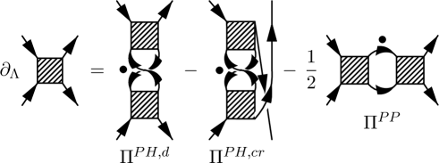
Figure 2: Diagrammatic representation of the flow equation for the two-particle vertex. The dots near the internal lines indicate differentiation of the propagator products with respect to the scale $\Lambda$.

was used in all previous studies of symmetry breaking from a fermionic flow.[10, 11, 12] The flow of the self-energy $\Sigma^{\Lambda}$ is determined by a tadpole contraction of the two-particle vertex $\Gamma^{(4)\Lambda}$ and the socalled single-scale propagator

$$S^{\Lambda}=\partial_{\Lambda}G^{\Lambda}|_{\Sigma^{\Lambda}\;{\rm fixed}}\;,$$ (3)

where $G^{\Lambda}$ is the infrared regularized propagator. The latter is defined by $(G^{\Lambda})^{-1}=\Gamma^{(2)\Lambda}+R^{\Lambda}$ with a suitable regulator function $R^{\Lambda}$. The flow of the two-particle vertex $\Gamma^{(4)\Lambda}$ is determined by a one-loop diagram involving $\Gamma^{(4)\Lambda}$ itself and the total cutoff derivative of the regularized propagator

$$\partial_{\Lambda}G^{\Lambda}=S^{\Lambda}-G^{\Lambda}(\partial_{\Lambda}\Sigma^{\Lambda})G^{\Lambda}\;.$$ (4)

The truncated system of flow equations described in Figs. 1 and 2 has the merit of solving mean-field models such as the reduced BCS model [10] and the reduced charged density wave model [11] exactly.

We now specify to singlet superconductivity, where the continuous $U(1)$ symmetry associated with charge conservation is spontaneously broken, while spin-rotation invariance remains conserved. It is useful to use Nambu spinors $\phi_{ks}$ and $\bar{\phi}_{ks}$ instead of $\psi_{k\sigma}$ and $\bar{\psi}_{k\sigma}$ as a basis. The two basis sets are related by

$$\bar{\phi}_{k+}=\bar{\psi}_{k\uparrow},\quad\phi_{k+}=\psi_{k\uparrow},\quad\bar{\phi}_{k-}=\psi_{-k\downarrow},\quad\phi_{k-}=\bar{\psi}_{-k\downarrow}\;.$$ (5)

The effective action as a functional of the Nambu fields, truncated beyond two-particle terms, has the form

$$\Gamma^{\Lambda}[\phi,\bar{\phi}] = \Gamma^{(0)\Lambda}+\sum_{k}\sum_{s_{1},s_{2}}\Gamma_{s_{1}s_{2}}^{(2)\Lambda}(k)\,\bar{\phi}_{ks_{1}}\phi_{ks_{2}}$$ (6)

$$+ \frac{1}{4}\sum_{k_{1},\dots,k_{4}}\sum_{s_{1},\dots,s_{4}}\Gamma_{s_{1}s_{2}s_{3}s_{4}}^{(4)\Lambda}(k_{1},k_{2},k_{3},k_{4})\,\bar{\phi}_{k_{1}s_{1}}\bar{\phi}_{k_{2}s_{2}}\phi_{k_{3}s_{3}}\phi_{k_{4}s_{4}}\;,$$

where $\Gamma^{(0)\Lambda}$ yields the grandcanonical potential. Due to spin-rotation invariance only terms with an equal number of $\phi$ and $\bar{\phi}$ fields contribute. The regularized Nambu propagator ${\bf G}^{\Lambda}$ is related to ${\bf\Gamma}^{(2)\Lambda}$ by $({\bf G}^{\Lambda})^{-1}={\bf\Gamma}^{(2)\Lambda}+{\bf R}^{\Lambda}$, and can be written as a $2\times 2$ matrix of the form

$${\bf G}^{\Lambda}(k)=\left(\begin{array}[]{cc}G_{++}^{\Lambda}(k)&G_{+-}^{\Lambda}(k)\\ G_{-+}^{\Lambda}(k)&G_{--}^{\Lambda}(k)\end{array}\right)=\left(\begin{array}[]{cc}G^{\Lambda}(k)&F^{\Lambda}(k)\\ F^{*\Lambda}(k)&-G^{\Lambda}(-k)\end{array}\right)\;.$$ (7)

Note that the anomalous propagator $F^{\Lambda}(k)$ is a symmetric function of $k_{0}$ and ${\bf k}$, due to spin-rotation and reflection invariance.

For a singlet superconductor, the flow equation for the Nambu self-energy ${\bf\Sigma}$, shown graphically in Fig. 1, is given by

$$\frac{d}{d\Lambda}\Sigma_{s_{1}s_{2}}^{\Lambda}(k)=-\sum_{k}\sum_{s_{3},s_{4}}S_{s_{4}s_{3}}^{\Lambda}(k^{\prime})\Gamma^{(4)\Lambda}_{s_{1}s_{3}s_{4}s_{2}}(k,k^{\prime},k^{\prime},k)\;,$$ (8)

and the flow equation for the Nambu vertex (Fig. 2) reads

$$\frac{d}{d\Lambda}\Gamma^{(4)\Lambda}_{s_{1}s_{2}s_{3}s_{4}}(k_{1},k_{2},k_{3},k_{4}) = \Pi^{PH,d}_{s_{1}s_{2}s_{3}s_{4}}(k_{1},k_{2},k_{3},k_{4})-\Pi^{PH,cr}_{s_{1}s_{2}s_{3}s_{4}}(k_{1},k_{2},k_{3},k_{4})$$ (9)

$$- \frac{1}{2}\Pi^{PP}_{s_{1}s_{2}s_{3}s_{4}}(k_{1},k_{2},k_{3},k_{4})\;,$$

where

$$\Pi^{PH,d}_{s_{1}s_{2}s_{3}s_{4}}(k_{1},k_{2},k_{3},k_{4}) = \sum_{p,q}\sum_{s^{\prime}_{1},\dots,s^{\prime}_{4}}\frac{d}{d\Lambda}[G^{\Lambda}_{s^{\prime}_{1}s^{\prime}_{2}}(p)G^{\Lambda}_{s^{\prime}_{3}s^{\prime}_{4}}(q)]$$ (10)

$$\times \Gamma^{(4)\Lambda}_{s_{1}s^{\prime}_{2}s^{\prime}_{3}s_{4}}(k_{1},p,q,k_{4})\Gamma^{(4)\Lambda}_{s^{\prime}_{4}s_{2}s_{3}s^{\prime}_{1}}(q,k_{2},k_{3},p)\;,$$

$$\Pi^{PH,cr}_{s_{1}s_{2}s_{3}s_{4}}(k_{1},k_{2},k_{3},k_{4}) = \sum_{p,q}\sum_{s^{\prime}_{1},\dots,s^{\prime}_{4}}\frac{d}{d\Lambda}[G^{\Lambda}_{s^{\prime}_{1}s^{\prime}_{2}}(p)G^{\Lambda}_{s^{\prime}_{3}s^{\prime}_{4}}(q)]$$ (11)

$$\times \Gamma^{(4)\Lambda}_{s_{2}s^{\prime}_{2}s^{\prime}_{3}s_{4}}(k_{2},p,q,k_{4})\Gamma^{(4)\Lambda}_{s^{\prime}_{4}s_{1}s_{3}s^{\prime}_{1}}(q,k_{1},k_{3},p)\;,$$

$$\Pi^{PP}_{s_{1}s_{2}s_{3}s_{4}}(k_{1},k_{2},k_{3},k_{4}) = \sum_{p,q}\sum_{s^{\prime}_{1},\dots,s^{\prime}_{4}}\frac{d}{d\Lambda}[G^{\Lambda}_{s^{\prime}_{1}s^{\prime}_{2}}(p)G^{\Lambda}_{s^{\prime}_{3}s^{\prime}_{4}}(q)]$$ (12)

$$\times \Gamma^{(4)\Lambda}_{s_{1}s_{2}s^{\prime}_{3}s^{\prime}_{1}}(k_{1},k_{2},q,p)\Gamma^{(4)\Lambda}_{s^{\prime}_{2}s^{\prime}_{4}s_{3}s_{4}}(p,q,k_{3},k_{4})\;.$$

Note that the particle-particle terms in the Nambu representation contain particle-hole contributions in the original fermion basis and vice versa. In particular, the original particle-particle contribution driving the superconducting instability is contained in the Nambu particle-hole diagrams.

We assume translation invariance such that the one-particle propagator and self-energy depend only on a single energy and momentum variable $k$, while the two-particle quantities are non-zero only if $k_{1}+k_{2}=k_{3}+k_{4}$, and can therefore be parametrized by three independent energy and momentum variables.

3 Constraints from symmetries

In this section we exploit the available symmetries to reduce the number of independent components of the two-particle vertex in the superconducting phase to a minimum. In any case, the effective action is invariant under translations, spin rotations and spatial inversions. In most singlet superconductors, also time reversal invariance remains unbroken.

In addition to the normal interaction involving two creation and two annihilation operators ($\bar{\psi}\bar{\psi}\psi\psi$) there are also anomalous vertices corresponding to operator products $\bar{\psi}\bar{\psi}\bar{\psi}\bar{\psi}$ + conjugate and $\bar{\psi}\bar{\psi}\bar{\psi}\psi$ + conjugate.[10, 12] We now write down manifestly spin-rotation invariant forms for each of these terms in the $\psi$-basis, and then translate to the Nambu representation.

A spin-rotation invariant normal interaction can be written as [15]

$$\Gamma^{(2+2)}[\psi,\bar{\psi}] = \frac{1}{4}\sum_{k_{i},\sigma_{i}}\left[V(k_{1},k_{2},k_{3},k_{4})\delta_{\sigma_{1}\sigma_{4}}\delta_{\sigma_{2}\sigma_{3}}-V(k_{1},k_{2},k_{4},k_{3})\delta_{\sigma_{1}\sigma_{3}}\delta_{\sigma_{2}\sigma_{4}}\right]$$ (13)

$$\times \bar{\psi}_{k_{1}\sigma_{1}}\bar{\psi}_{k_{2}\sigma_{2}}\psi_{k_{3}\sigma_{3}}\psi_{k_{4}\sigma_{4}}\;.$$

Here and in the remainder of this section we suppress the superscript $\Lambda$ denoting the scale dependence. Alternatively one may write $\Gamma^{(2+2)}[\psi,\bar{\psi}]$ as a sum of a spin singlet and a spin triplet component [4]

$$\Gamma^{(2+2)}[\psi,\bar{\psi}] = \frac{1}{4}\sum_{k_{i},\sigma_{i}}\left[V^{S}(k_{1},k_{2},k_{3},k_{4})S_{\sigma_{1}\sigma_{2}\sigma_{3}\sigma_{4}}+V^{T}(k_{1},k_{2},k_{3},k_{4})T_{\sigma_{1}\sigma_{2}\sigma_{3}\sigma_{4}}\right]$$ (14)

$$\times \bar{\psi}_{k_{1}\sigma_{1}}\bar{\psi}_{k_{2}\sigma_{2}}\psi_{k_{3}\sigma_{3}}\psi_{k_{4}\sigma_{4}}\;,$$

where $S_{\sigma_{1}\sigma_{2}\sigma_{3}\sigma_{4}}=\frac{1}{2}(\delta_{\sigma_{1}\sigma_{4}}\delta_{\sigma_{2}\sigma_{3}}-\delta_{\sigma_{1}\sigma_{3}}\delta_{\sigma_{2}\sigma_{4}})$, $T_{\sigma_{1}\sigma_{2}\sigma_{3}\sigma_{4}}=\frac{1}{2}(\delta_{\sigma_{1}\sigma_{4}}\delta_{\sigma_{2}\sigma_{3}}+\delta_{\sigma_{1}\sigma_{3}}\delta_{\sigma_{2}\sigma_{4}})$, and

$$V^{S}(k_{1},k_{2},k_{3},k_{4}) = V(k_{1},k_{2},k_{3},k_{4})+V(k_{1},k_{2},k_{4},k_{3})\;,$$ (15)

$$V^{T}(k_{1},k_{2},k_{3},k_{4}) = V(k_{1},k_{2},k_{3},k_{4})-V(k_{1},k_{2},k_{4},k_{3})\;.$$ (16)

Time reversal invariance [17] and charge conjugation (corresponding to hermiticity of the underlying Hamiltionian) yield the following relations for $V(k_{1},k_{2},k_{3},k_{4})$:

$$V(k_{1},k_{2},k_{3},k_{4}) = V(k_{4}^{\cal T},k_{3}^{\cal T},k_{2}^{\cal T},k_{1}^{\cal T})\quad\mbox{(time reversal)}\;,$$ (17)

$$V(k_{1},k_{2},k_{3},k_{4}) = V^{*}(k_{4}^{*},k_{3}^{*},k_{2}^{*},k_{1}^{*})\quad\;\,\mbox{(charge conjugation)}\;,$$ (18)

where $k^{\cal T}=(k_{0},-{\bf k})$ and $k^{*}=(-k_{0},{\bf k})$, and the same for $V^{S}$ and $V^{T}$. Note that spatial inversions also transform $k$ to $k^{\cal T}$, but without permuting the momenta in $V(k_{1},k_{2},k_{3},k_{4})$. The invariance of the action under the exchange of identical particles yields separate symmetry relations for $V^{S}$ and $V^{T}$ under $k_{1}\leftrightarrow k_{2}$ and $k_{3}\leftrightarrow k_{4}$:

$$V^{S}(k_{1},k_{2},k_{3},k_{4})= \phantom{-}V^{S}(k_{2},k_{1},k_{3},k_{4})\, =\phantom{-}V^{S}(k_{1},k_{2},k_{4},k_{3})\;,$$ (19)

$$V^{T}(k_{1},k_{2},k_{3},k_{4})= -V^{T}(k_{2},k_{1},k_{3},k_{4})\, =-V^{T}(k_{1},k_{2},k_{4},k_{3})\;,$$ (20)

while $V$ obeys only

$$V(k_{1},k_{2},k_{3},k_{4})=V(k_{2},k_{1},k_{4},k_{3})\;.$$ (21)

A spin-rotation invariant ansatz for the anomalous interactions can be constructed systematically by requiring that commutators with the three components of the total spin operator vanish.

A spin-rotation invariant anomalous interaction involving four creation or four annihilation operators can be written in the form

$$\Gamma^{(4+0)}[\psi,\bar{\psi}]=$$

$$\frac{1}{8}\sum_{k_{i}} \Big{\{}W^{S}(k_{1},k_{2},k_{3},k_{4})(\bar{\psi}_{k_{1}\uparrow}\bar{\psi}_{k_{2}\downarrow}-\bar{\psi}_{k_{1}\downarrow}\bar{\psi}_{k_{2}\uparrow})(\bar{\psi}_{k_{3}\uparrow}\bar{\psi}_{k_{4}\downarrow}-\bar{\psi}_{k_{3}\downarrow}\bar{\psi}_{k_{4}\uparrow})$$

$$- \,W^{T}(k_{1},k_{2},k_{3},k_{4})\big{[}(\bar{\psi}_{k_{1}\uparrow}\bar{\psi}_{k_{2}\downarrow}+\bar{\psi}_{k_{1}\downarrow}\bar{\psi}_{k_{2}\uparrow})(\bar{\psi}_{k_{3}\uparrow}\bar{\psi}_{k_{4}\downarrow}+\bar{\psi}_{k_{3}\downarrow}\bar{\psi}_{k_{4}\uparrow})$$ (22)

$$-2(\bar{\psi}_{k_{1}\uparrow}\bar{\psi}_{k_{2}\uparrow}\bar{\psi}_{k_{3}\downarrow}\bar{\psi}_{k_{4}\downarrow}+\bar{\psi}_{k_{1}\downarrow}\bar{\psi}_{k_{2}\downarrow}\bar{\psi}_{k_{3}\uparrow}\bar{\psi}_{k_{4}\uparrow})\big{]}+{\rm conj.}\Big{\}}\;,$$

consisting of a singlet ($S$) and a triplet ($T$) term, which are separately invariant under spin rotations. Charge conjugated terms are denoted by ”conj.”. Time reversal invariance yields a relation between $W^{S,T}$ and $W^{S,T*}$, which assumes the simple form

$$W^{S,T*}(k_{1},k_{2},k_{3},k_{4})=W^{S,T}(-k_{1},-k_{2},-k_{3},-k_{4})\;,$$ (23)

if the order parameter (gap function) is chosen real. Furthermore, the functions $W^{S}(k_{1},k_{2},k_{3},k_{4})$ and $W^{T}(k_{1},k_{2},k_{3},k_{4})$ are symmetric and antisymmetric under the exchange $k_{1}\leftrightarrow k_{2}$ or $k_{3}\leftrightarrow k_{4}$, respectively, and symmetric under the simultaneous exchange $k_{1}\leftrightarrow k_{3}$ and $k_{2}\leftrightarrow k_{4}$:

$$W^{S}(k_{1},k_{2},k_{3},k_{4}) = W^{S}(k_{2},k_{1},k_{3},k_{4})=W^{S}(k_{1},k_{2},k_{4},k_{3})$$ (24)

$$= W^{S}(k_{3},k_{4},k_{1},k_{2})\;,$$

$$W^{T}(k_{1},k_{2},k_{3},k_{4}) = -W^{T}(k_{2},k_{1},k_{3},k_{4})=-W^{T}(k_{1},k_{2},k_{4},k_{3})$$ (25)

$$= W^{T}(k_{3},k_{4},k_{1},k_{2})\;.$$

Finally, a spin-rotation invariant anomalous interaction with three creation and one annihilation operators, or vice versa, can be written as

$$\Gamma^{(3+1)}[\psi,\bar{\psi}] = \frac{1}{2}\sum_{k_{i}}\Big{\{}X^{S}(k_{1},k_{2},k_{3},k_{4})\sum_{\sigma}\bar{\psi}_{k_{1}\sigma}(\bar{\psi}_{k_{2}\uparrow}\bar{\psi}_{k_{3}\downarrow}-\bar{\psi}_{k_{2}\downarrow}\bar{\psi}_{k_{3}\uparrow})\psi_{k_{4}\sigma}$$ (26)

$$+\;X^{T}(k_{1},k_{2},k_{3},k_{4})\Big{[}\sum_{\sigma}\epsilon_{\sigma}\bar{\psi}_{k_{1}\sigma}(\bar{\psi}_{k_{2}\uparrow}\bar{\psi}_{k_{3}\downarrow}+\bar{\psi}_{k_{2}\downarrow}\bar{\psi}_{k_{3}\uparrow})\psi_{k_{4}\sigma}$$

$$\quad+\;2(\bar{\psi}_{k_{1}\uparrow}\bar{\psi}_{k_{2}\downarrow}\bar{\psi}_{k_{3}\downarrow}\psi_{k_{4}\downarrow}-\bar{\psi}_{k_{1}\downarrow}\bar{\psi}_{k_{2}\uparrow}\bar{\psi}_{k_{3}\uparrow}\psi_{k_{4}\uparrow})\Big{]}+{\rm conj.}\Big{\}}\;,$$

where $\epsilon_{\uparrow}=1$ and $\epsilon_{\downarrow}=-1$. The terms with the coefficients $X^{S}$ and $X^{T}$ are separately spin-rotation invariant. Time reversal invariance yields the relation

$$X^{S,T*}(k_{1},k_{2},k_{3},k_{4})=X^{S,T}(-k_{1},-k_{2},-k_{3},-k_{4})$$ (27)

for a real choice of the order parameter. Invariance under particle exchange yields

$$X^{S}(k_{1},k_{2},k_{3},k_{4}) = \phantom{-}X^{S}(k_{1},k_{3},k_{2},k_{4})\;,$$

$$X^{T}(k_{1},k_{2},k_{3},k_{4}) = -X^{T}(k_{1},k_{3},k_{2},k_{4})\;.$$ (28)

To express the two-particle interaction in terms of Nambu fields, it is convenient to collect the 16 components of the Nambu vertex $\Gamma_{s_{1}s_{2}s_{3}s_{4}}^{(4)}$ in a $4\times 4$ matrix

$${\bf\Gamma}^{(4)}=\left(\begin{array}[]{cccc}\Gamma_{++++}^{(4)}&\Gamma_{++-+}^{(4)}&\Gamma_{+-++}^{(4)}&\Gamma_{+--+}^{(4)}\\[5.69054pt] \Gamma_{+++-}^{(4)}&\Gamma_{++--}^{(4)}&\Gamma_{+-+-}^{(4)}&\Gamma_{+---}^{(4)}\\[5.69054pt] \Gamma_{-+++}^{(4)}&\Gamma_{-+-+}^{(4)}&\Gamma_{--++}^{(4)}&\Gamma_{---+}^{(4)}\\[5.69054pt] \Gamma_{-++-}^{(4)}&\Gamma_{-+--}^{(4)}&\Gamma_{--+-}^{(4)}&\Gamma_{----}^{(4)}\end{array}\right)\quad.$$ (29)

Note that the rows in this matrix are labelled by $s_{1}$ and $s_{4}$, while columns are labelled by $s_{2}$ and $s_{3}$. With this assignment the Bethe-Salpeter equation yielding the exact Nambu vertex in reduced (mean-field) models can be written as a matrix equation. Translating the spin-rotation invariant structure of the various interaction terms described above to the Nambu representation, one obtains a Nambu vertex of the following form

$${\bf\Gamma}^{(4)}(k_{1},k_{2},k_{3},k_{4})=\hskip 298.75394pt$$

$$\left(\!\begin{array}[]{cccc}V^{T}(k_{1},k_{2},k_{3},k_{4})&X(k_{1},k_{2},k_{3},k_{4})&X^{*}(k^{*}_{4},k^{*}_{3},k^{*}_{2},k^{*}_{1})&\!\!-V(k_{1},\bar{k}_{3},\bar{k}_{2},k_{4})\\[5.69054pt] \!\!-X(k_{1},k_{2},k_{4},k_{3})&W(k_{1},k_{2},k_{3},k_{4})&V(k_{1},\bar{k}_{4},\bar{k}_{2},k_{3})&X^{*}(k_{4},k_{3},k_{1},k_{2})\\[5.69054pt] \!\!-X^{*}(k^{*}_{3},k^{*}_{4},k^{*}_{2},k^{*}_{1})&V^{*}(k_{1},\bar{k}_{4},\bar{k}_{2},k_{3})&W^{*}(k^{*}_{4},k^{*}_{3},k^{*}_{2},k^{*}_{1})&X(k^{*}_{2},k^{*}_{1},k^{*}_{3},k^{*}_{4})\\[5.69054pt] \!\!-V^{*}(k_{1},\bar{k}_{3},\bar{k}_{2},k_{4})&\!\!-X^{*}(k_{4},k_{3},k_{2},k_{1})&\!\!-X(k^{*}_{1},k^{*}_{2},k^{*}_{3},k^{*}_{4})&V^{T*}(k_{1},k_{2},k_{3},k_{4})\end{array}\!\!\right)$$ (34)

where $\bar{k}=-k$. The matrix elements $W$ and $X$ are related to the anomalous (4+0) and (3+1) interactions, respectively:

$$W(k_{1},k_{2},k_{3},k_{4}) = W^{S}(k_{1},-k_{4},-k_{3},k_{2})-W^{S}(k_{1},-k_{3},-k_{4},k_{2})$$ (36)

$$+ W^{T}(k_{1},-k_{4},-k_{3},k_{2})-W^{T}(k_{1},-k_{3},-k_{4},k_{2})$$

$$+ 2W^{T}(k_{1},k_{2},-k_{3},-k_{4})\;,$$

$$X(k_{1},k_{2},k_{3},k_{4}) = X^{S}(k_{1},k_{2},-k_{3},k_{4})-X^{S}(k_{2},k_{1},-k_{3},k_{4})$$ (37)

$$+ X^{T}(k_{1},k_{2},-k_{3},k_{4})-X^{T}(k_{2},k_{1},-k_{3},k_{4})$$

$$+ 2X^{T}(-k_{3},k_{2},k_{1},k_{4})\;.$$

The functions $W$ and $X$ obey the following relations under exchange of variables:

$$W(k_{1},k_{2},k_{3},k_{4}) = -W(k_{2},k_{1},k_{3},k_{4})=-W(k_{1},k_{2},k_{4},k_{3})$$ (38)

$$= \phantom{-}W(-k_{4},-k_{3},-k_{2},-k_{1})\;,$$

$$X(k_{1},k_{2},k_{3},k_{4}) = -X(k_{2},k_{1},k_{3},k_{4})\;.$$ (39)

In summary, by fully exploiting the available symmetries, in particular spin-rotation invariance, the number of independent functions parametrizing the Nambu vertex could be reduced substantially compared to what one gets by exploiting only the conservation of the $z$-component of the spin.[12]

4 Reduced BCS plus forward scattering model

In this section we consider a model with reduced interactions in the Cooper and forward scattering channels. The truncated flow equations described in §2 yield the exact flow for that model. By analyzing the flow we gain insight into the role of the various anomalous interactions and their singularities at and below the critical scale for superconductivity.

The model is defined by the following action

$$S[\psi,\bar{\psi}]=S_{0}[\psi,\bar{\psi}]+V_{sc}[\psi,\bar{\psi}]+V_{c}[\psi,\bar{\psi}]+V_{s}[\psi,\bar{\psi}]\;,$$ (40)

consisting of a quadratic and three interaction terms.

$$S_{0}[\psi,\bar{\psi}]=\sum_{k,\sigma}(-ik_{0}+\xi_{{\bf k}})\bar{\psi}_{k\sigma}\psi_{k\sigma}+\sum_{k}\left(\Delta^{(0)}(k)\bar{\psi}_{k\uparrow}\bar{\psi}_{-k\downarrow}+\Delta^{(0)*}(k)\psi_{-k\downarrow}\psi_{k\uparrow}\right)$$ (41)

contains the kinetic energy and an external pairing field $\Delta^{(0)}$, while $V_{sc}$, $V_{c}$ and $V_{s}$ are reduced interactions in the Cooper (superconducting), forward charge, and forward spin (magnetic) channel, respectively:

$$V_{sc}[\psi,\bar{\psi}] = \sum_{k_{1},k_{2}}V^{(0)}(k_{1},k_{2})\,\bar{\psi}_{k_{1}\uparrow}\bar{\psi}_{-k_{1}\downarrow}\psi_{-k_{2}\downarrow}\psi_{k_{2}\uparrow}\;,$$ (42)

$$V_{c}[\psi,\bar{\psi}] = \frac{1}{2}\sum_{k_{1},k_{2}}\sum_{\sigma_{1},\sigma_{2}}F^{(0)}_{c}(k_{1},k_{2})\,\bar{\psi}_{k_{1}\sigma_{1}}\bar{\psi}_{k_{2}\sigma_{2}}\psi_{k_{2}\sigma_{2}}\psi_{k_{1}\sigma_{1}}\;,$$ (43)

$$V_{s}[\psi,\bar{\psi}] = \frac{1}{2}\sum_{k_{1},k_{2}}\sum_{\sigma_{1},\sigma^{\prime}_{1}}\sum_{\sigma_{2},\sigma^{\prime}_{2}}F^{(0)}_{s}(k_{1},k_{2})\left(\vec{\tau}_{\sigma_{1}\sigma^{\prime}_{1}}\cdot\vec{\tau}_{\sigma_{2}\sigma^{\prime}_{2}}\right)\,\bar{\psi}_{k_{1}\sigma_{1}}\bar{\psi}_{k_{2}\sigma_{2}}\psi_{k_{2}\sigma^{\prime}_{2}}\psi_{k_{1}\sigma^{\prime}_{1}}\;,\hskip 28.45274pt$$ (44)

where $\vec{\tau}=(\tau^{x},\tau^{y},\tau^{z})$ is the vector formed by the three Pauli matrices. The coupling functions $V^{(0)}(k_{1},k_{2})$, $F^{(0)}_{c}(k_{1},k_{2})$ and $F^{(0)}_{s}(k_{1},k_{2})$ are arbitrary functions of $k_{1}$ and $k_{2}$. The interaction terms correspond to a spin-rotation invariant normal vertex of the form (13) with

$$V(k_{1},k_{2},k_{3},k_{4}) = V^{(0)}(k_{1},k_{4})\delta_{k_{1},-k_{2}}\delta_{k_{3},-k_{4}}+F^{(0)}_{c}(k_{1},k_{2})\delta_{k_{1},k_{4}}\delta_{k_{2},k_{3}}$$ (45)

$$- F^{(0)}_{s}(k_{1},k_{2})(\delta_{k_{1},k_{4}}\delta_{k_{2},k_{3}}+2\delta_{k_{1},k_{3}}\delta_{k_{2},k_{4}})\;.$$

The pairing field $\Delta^{(0)}$ breaks the $U(1)$ charge symmetry explicitly. Spontaneous symmetry breaking is obtained in the limit $\Delta^{(0)}\to 0$. The model (40) is a generalization of the reduced BCS model, where only $V_{sc}$ contributes, whose flow was discussed extensively in Ref. Salmhofer04. A special version of the model (40) with $V_{s}=0$ was solved by a summation of all contributing Feynman diagrams in Ref. Gersch07.

4.1 Exact integral equations and Ward identity

Due to the restricted momentum dependence of the interaction terms, all contributions to $\Gamma^{(2)\Lambda}$ and $\Gamma^{(4)\Lambda}$ discarded in the truncation described in §2 vanish in the thermodynamic limit. This follows from a straightforward generalization of the arguments given in Ref. Salmhofer04. The constrained momentum dependence of the interactions leads to the following constraints on the external momenta of the various one-loop contributions to the flow of the Nambu vertex $\Gamma^{(4)\Lambda}_{s_{1}s_{2}s_{3}s_{4}}(k_{1},k_{2},k_{3},k_{4})$, Eq. (9):

$$\Pi^{PH,d}_{s_{1}s_{2}s_{3}s_{4}}(k_{1},k_{2},k_{3},k_{4}) \propto \delta_{k_{1},k_{4}}\delta_{k_{2},k_{3}}\;,$$

$$\Pi^{PH,cr}_{s_{1}s_{2}s_{3}s_{4}}(k_{1},k_{2},k_{3},k_{4}) \propto \delta_{k_{1},k_{3}}\delta_{k_{2},k_{4}}\;,$$

$$\Pi^{PP}_{s_{1}s_{2}s_{3}s_{4}}(k_{1},k_{2},k_{3},k_{4}) \propto \delta_{k_{1},-k_{2}}\delta_{k_{3},-k_{4}}\;.$$ (46)

It is sufficient to consider the flow equation for the Nambu vertex with $k_{1}=k_{4}$ and $k_{2}=k_{3}$, since the non-vanishing matrix elements for other choices of momenta follow from symmetries. Choosing $k_{1}=k_{4}=:k$ and $k_{2}=k_{3}=:k^{\prime}$, only the direct particle-hole term contributes and the flow equation simplifies to

$$\frac{d}{d\Lambda}\Gamma^{(4)\Lambda}_{s_{1}s_{2}s_{3}s_{4}}(k,k^{\prime},k^{\prime},k)= \hskip-56.9055pt\Pi^{PH,d}_{s_{1}s_{2}s_{3}s_{4}}(k,k^{\prime},k^{\prime},k)=$$

$$\sum_{p,s^{\prime}_{i}}\frac{d}{d\Lambda}[G^{\Lambda}_{s^{\prime}_{1}s^{\prime}_{2}}(p)G^{\Lambda}_{s^{\prime}_{3}s^{\prime}_{4}}(p)] \Gamma^{(4)\Lambda}_{s_{1}s^{\prime}_{2}s^{\prime}_{3}s_{4}}(k,p,p,k)\Gamma^{(4)\Lambda}_{s^{\prime}_{4}s_{2}s_{3}s^{\prime}_{1}}(p,k^{\prime},k^{\prime},p)\;.$$ (47)

This differential equation is equivalent to the Bethe-Salpeter-like integral equation

$$\hskip-14.22636pt\Gamma^{(4)\Lambda}_{s_{1}s_{2}s_{3}s_{4}}(k,k^{\prime},k^{\prime},k) = \Gamma^{(4)\Lambda_{0}}_{s_{1}s_{2}s_{3}s_{4}}(k,k^{\prime},k^{\prime},k)$$

$$+\sum_{p,s^{\prime}_{i}} \hskip-14.22636ptG^{\Lambda}_{s^{\prime}_{1}s^{\prime}_{2}}(p)G^{\Lambda}_{s^{\prime}_{3}s^{\prime}_{4}}(p)\Gamma^{(4)\Lambda_{0}}_{s_{1}s^{\prime}_{2}s^{\prime}_{3}s_{4}}(k,p,p,k)\Gamma^{(4)\Lambda}_{s^{\prime}_{4}s_{2}s_{3}s^{\prime}_{1}}(p,k^{\prime},k^{\prime},p)$$ (48)

summing up all Nambu particle-hole ladder diagrams. Note that $G^{\Lambda_{0}}=0$. Inserting this implicit solution for $\Gamma^{(4)\Lambda}$ into the flow equation (8) for the self-energy, and using the relation ${\bf S}^{\Lambda}=\dot{\bf G}^{\Lambda}+{\bf G}^{\Lambda}\dot{\bf\Sigma}^{\Lambda}{\bf G}^{\Lambda}$, the flow of the self-energy can be integrated, yielding

$$\Sigma^{\Lambda}_{s_{1}s_{2}}(k)-\Sigma^{\Lambda_{0}}_{s_{1}s_{2}}(k)=-\sum_{k^{\prime}}\sum_{s_{3},s_{4}}G^{\Lambda}_{s_{4}s_{3}}(k^{\prime})\Gamma^{(4)\Lambda_{0}}_{s_{1}s_{3}s_{4}s_{2}}(k,k^{\prime},k^{\prime},k)\;,$$ (49)

with the bare Nambu vertex on the right hand side. This is just the familiar mean-field equation for the self-energy, which is exact for the reduced model (40).

The exact solution determined by Eqs. (4.1) and (49) fulfils the Ward identity following from global charge conservation,[10]

$$\Delta^{\Lambda}(k)-\Delta^{(0)}(k) = \sum_{k^{\prime}}\sum_{s,s^{\prime}}\left[\Delta^{(0)}(k^{\prime})G^{\Lambda}_{s+}(k^{\prime})G^{\Lambda}_{-s^{\prime}}(k^{\prime})-\Delta^{(0)*}(k^{\prime})G^{\Lambda}_{s-}(k^{\prime})G^{\Lambda}_{+s^{\prime}}(k^{\prime})\right]$$ (50)

$$\times\Gamma^{(4)\Lambda}_{+s^{\prime}s-}(k,k^{\prime},k^{\prime},k)\;,$$

which connects the anomalous self-energy $\Sigma^{\Lambda}_{+-}(k)=\Delta^{\Lambda}(k)$ with the two-particle vertex. The Ward identity implies that some components of the Nambu vertex diverge in case of spontaneous symmetry breaking ($\Delta^{\Lambda}$ finite for $\Delta^{(0)}\to 0$).

4.2 Explicit solution and singularities of Nambu vertex

An explicit solution of the Bethe-Salpeter equation (4.1) for the Nambu vertex can be obtained for the case of separable momentum dependences of the interaction terms in the reduced model. In this special case the singularities of the various components of the Nambu vertex become particularly transparent.

Using the $4\times 4$ matrix representation of the Nambu vertex, Eq. (29), one can write the integral equation (4.1) in matrix form as

$${\bf\Gamma}^{(4)\Lambda}(k,k^{\prime})={\bf\Gamma}^{(4)\Lambda_{0}}(k,k^{\prime})+\sum_{p}{\bf\Gamma}^{(4)\Lambda_{0}}(k,p)\,{\bf L}^{\Lambda}(p)\,{\bf\Gamma}^{(4)\Lambda}(p,k^{\prime})\;,$$ (51)

where ${\bf\Gamma}^{(4)\Lambda}(k,k^{\prime})={\bf\Gamma}^{(4)\Lambda}(k,k^{\prime},k^{\prime},k)$ and ${\bf L}^{\Lambda}$ is the $4\times 4$ matrix defined by

$${\bf L}^{\Lambda}=\left(\begin{array}[]{cccc}G^{\Lambda}_{++}G^{\Lambda}_{++}&G^{\Lambda}_{-+}G^{\Lambda}_{++}&G^{\Lambda}_{++}G^{\Lambda}_{+-}&G^{\Lambda}_{-+}G^{\Lambda}_{+-}\\[5.69054pt] G^{\Lambda}_{++}G^{\Lambda}_{-+}&G^{\Lambda}_{-+}G^{\Lambda}_{-+}&G^{\Lambda}_{++}G^{\Lambda}_{--}&G^{\Lambda}_{-+}G^{\Lambda}_{--}\\[5.69054pt] G^{\Lambda}_{+-}G^{\Lambda}_{++}&G^{\Lambda}_{--}G^{\Lambda}_{++}&G^{\Lambda}_{+-}G^{\Lambda}_{+-}&G^{\Lambda}_{--}G^{\Lambda}_{+-}\\[5.69054pt] G^{\Lambda}_{+-}G^{\Lambda}_{-+}&G^{\Lambda}_{--}G^{\Lambda}_{-+}&G^{\Lambda}_{+-}G^{\Lambda}_{--}&G^{\Lambda}_{--}G^{\Lambda}_{--}\end{array}\right)\quad.$$ (52)

The bare Nambu vertex ${\bf\Gamma}^{(4)\Lambda_{0}}(k,k^{\prime})$ corresponding to the reduced interaction in Eq. (45) has the form

$${\bf\Gamma}^{(4)\Lambda_{0}}(k,k^{\prime})=\left(\begin{array}[]{cccc}F^{(0)}_{1}(k,k^{\prime})&0&0&F^{(0)}_{2}(k,k^{\prime})\\[5.69054pt] 0&0&V^{(0)}(k,k^{\prime})&0\\[5.69054pt] 0&V^{(0)*}(k,k^{\prime})&0&0\\[5.69054pt] F^{(0)*}_{2}(k,k^{\prime})&0&0&F^{(0)*}_{1}(k,k^{\prime})\end{array}\right)\;,$$ (53)

where

$$F^{(0)}_{1}(k,k^{\prime}) = F^{(0)}_{c}(k,k^{\prime})+F^{(0)}_{s}(k,k^{\prime})\;,$$

$$F^{(0)}_{2}(k,k^{\prime}) = F^{(0)}_{s}(k,-k^{\prime})-F^{(0)}_{c}(k,-k^{\prime})\;.$$ (54)

The structure of the full Nambu vertex ${\bf\Gamma}^{(4)\Lambda}(k,k^{\prime})$ is obtained by specializing the general form Eq. (3) to the case $k_{1}=k_{4}=k$ and $k_{2}=k_{3}=k^{\prime}$ as

$${\bf\Gamma}^{(4)\Lambda}(k,k^{\prime})=\left(\begin{array}[]{cccc}F^{\Lambda}_{1}(k,k^{\prime})&X^{\Lambda}(k,k^{\prime})&X^{\Lambda*}(k^{*},{k^{\prime}}^{*})&F^{\Lambda}_{2}(k,k^{\prime})\\[5.69054pt] X^{\Lambda}(k^{\prime},k)&W^{\Lambda}(k,k^{\prime})&V^{\Lambda}(k,k^{\prime})&-X^{\Lambda*}(k^{\prime},k)\\[5.69054pt] X^{\Lambda*}({k^{\prime}}^{*},k^{*})&V^{\Lambda*}(k,k^{\prime})&W^{\Lambda*}(k^{*},{k^{\prime}}^{*})&-X^{\Lambda}({k^{\prime}}^{*},k^{*})\\[5.69054pt] F^{\Lambda*}_{2}(k,k^{\prime})&-X^{\Lambda*}(k,k^{\prime})&-X^{\Lambda}(k^{*},{k^{\prime}}^{*})&F^{\Lambda*}_{1}(k,k^{\prime})\end{array}\right)\;.$$ (55)

In the following we assume that the bare coupling functions $V^{(0)}$, $F^{(0)}_{c}$, $F^{(0)}_{s}$, and the external pairing field $\Delta^{(0)}$ are real and frequency independent. Then ${\bf\Gamma}^{(4)\Lambda}(k,k^{\prime})$ and $\Delta^{\Lambda}(k)$ are also real and frequency independent, such that the complex conjugation operations in Eq. (55) can be omitted. The matrix products in the Bethe-Salpeter equation (4.1) can then be simplified considerably by employing the following orthogonal transformation

$${\bf U}=\frac{1}{\sqrt{2}}\left(\begin{array}[]{rrcc}1&0&0&1\\[5.69054pt] 0&1&1&0\\[5.69054pt] 0&-1&1&0\\[5.69054pt] -1&0&0&1\end{array}\right)\;.$$ (56)

The transformed vertex $\tilde{\bf\Gamma}^{(4)\Lambda}={\bf U}{\bf\Gamma}^{(4)\Lambda}{\bf U}^{T}$ has the form

$$\tilde{\bf\Gamma}^{(4)\Lambda}(k,k^{\prime})=\left(\begin{array}[]{cccc}F^{\Lambda}_{+}(k,k^{\prime})&0&0&0\\[5.69054pt] 0&A^{\Lambda}(k,k^{\prime})&0&-2X^{\Lambda}(k^{\prime},k)\\[5.69054pt] 0&0&-\Phi^{\Lambda}(k,k^{\prime})&0\\[5.69054pt] 0&-2X^{\Lambda}(k,k^{\prime})&0&F^{\Lambda}_{-}(k,k^{\prime})\end{array}\right)\;,$$ (57)

with the ”amplitude” ($A$) and ”phase” ($\Phi$) components

$$A^{\Lambda}(k,k^{\prime}) = V^{\Lambda}(k,k^{\prime})+W^{\Lambda}(k,k^{\prime})\;,$$

$$\Phi^{\Lambda}(k,k^{\prime}) = V^{\Lambda}(k,k^{\prime})-W^{\Lambda}(k,k^{\prime})\;,$$ (58)

and the linear combinations in the forward scattering channel

$$F^{\Lambda}_{\pm}(k,k^{\prime})=F^{\Lambda}_{1}(k,k^{\prime})\pm F^{\Lambda}_{2}(k,k^{\prime})\;.$$ (59)

The transformed bare vertex $\tilde{\bf\Gamma}^{(4)\Lambda_{0}}(k,k^{\prime})$ has only diagonal entries:

$$\tilde{\bf\Gamma}^{(4)\Lambda_{0}}(k,k^{\prime})=\left(\begin{array}[]{cccc}F^{(0)}_{+}(k,k^{\prime})&0&0&0\\[5.69054pt] 0&V^{(0)}(k,k^{\prime})&0&0\\[5.69054pt] 0&0&-V^{(0)}(k,k^{\prime})&0\\[5.69054pt] 0&0&0&F^{(0)}_{-}(k,k^{\prime})\end{array}\right)\;.$$ (60)

The frequency summed matrix ${\bf L}^{\Lambda}({\bf p})=\sum_{p_{0}}{\bf L}^{\Lambda}(p)$ also transforms to a simpler block matrix structure

$$\tilde{\bf L}^{\Lambda}({\bf p})=\left(\begin{array}[]{cccc}L^{\Lambda}_{f_{+}}({\bf p})&0&0&0\\[5.69054pt] 0&L^{\Lambda}_{a}({\bf p})&0&L^{\Lambda}_{x}({\bf p})\\[5.69054pt] 0&0&L^{\Lambda}_{\phi}({\bf p})&0\\[5.69054pt] 0&L^{\Lambda}_{x}({\bf p})&0&L^{\Lambda}_{f_{-}}({\bf p})\end{array}\right)\;,$$ (61)

where

$$L^{\Lambda}_{a}({\bf p}) = \sum_{p_{0}}[G^{\Lambda}_{+-}(p)]^{2}+G^{\Lambda}_{++}(p)G^{\Lambda}_{--}(p)\;,$$

$$L^{\Lambda}_{\phi}({\bf p}) = \sum_{p_{0}}[G^{\Lambda}_{+-}(p)]^{2}-G^{\Lambda}_{++}(p)G^{\Lambda}_{--}(p)\;,$$

$$L^{\Lambda}_{x}({\bf p}) = -2\sum_{p_{0}}G^{\Lambda}_{++}(p)G^{\Lambda}_{+-}(p)\;,$$

$$L^{\Lambda}_{f_{+}}({\bf p}) = \sum_{p_{0}}[G^{\Lambda}_{++}(p)]^{2}+[G^{\Lambda}_{+-}(p)]^{2}\;,$$

$$L^{\Lambda}_{f_{-}}({\bf p}) = \sum_{p_{0}}[G^{\Lambda}_{++}(p)]^{2}-[G^{\Lambda}_{+-}(p)]^{2}\;.$$ (62)

For an explicit solution, we now assume that the momentum dependences of the bare interactions factorize:

$$V^{(0)}(k,k^{\prime}) = g^{(0)}f_{sc}({\bf k})f_{sc}({\bf k}^{\prime})\;,$$

$$F^{(0)}_{c}(k,k^{\prime}) = g^{(0)}_{c}f_{c}({\bf k})f_{c}({\bf k}^{\prime})\;,$$

$$F^{(0)}_{s}(k,k^{\prime}) = g^{(0)}_{s}f_{s}({\bf k})f_{s}({\bf k}^{\prime})\;,$$ (63)

where $f_{sc}({\bf k})$, $f_{c}({\bf k})$, and $f_{s}({\bf k})$ are arbitrary reflection invariant form factors. Then the momentum dependences of the flowing interactions also factorize in the form

$$V^{\Lambda}(k,k^{\prime}) = g^{\Lambda}f_{sc}({\bf k})f_{sc}({\bf k}^{\prime})\;,$$

$$F^{\Lambda}_{-}(k,k^{\prime}) = 2g^{\Lambda}_{c}f_{c}({\bf k})f_{c}({\bf k}^{\prime})\;,$$

$$F^{\Lambda}_{+}(k,k^{\prime}) = 2g^{\Lambda}_{s}f_{s}({\bf k})f_{s}({\bf k}^{\prime})\;,$$

$$W^{\Lambda}(k,k^{\prime}) = g^{\Lambda}_{w}f_{sc}({\bf k})f_{sc}({\bf k}^{\prime})\;,$$

$$X^{\Lambda}(k,k^{\prime}) = g^{\Lambda}_{x}f_{c}({\bf k})f_{sc}({\bf k}^{\prime})\;,$$ (64)

and also the linear combinations $V^{\Lambda}\pm W^{\Lambda}$,

$$A^{\Lambda}(k,k^{\prime}) = g^{\Lambda}_{a}f_{sc}({\bf k})f_{sc}({\bf k}^{\prime})\;,$$

$$\Phi^{\Lambda}(k,k^{\prime}) = g^{\Lambda}_{\phi}f_{sc}({\bf k})f_{sc}({\bf k}^{\prime})\;,$$ (65)

with $g^{\Lambda}_{a}=g^{\Lambda}+g^{\Lambda}_{w}$ and $g^{\Lambda}_{\phi}=g^{\Lambda}-g^{\Lambda}_{w}$.

The momentum dependences on the right hand side of the integral equation (4.1) now factorize, and the momentum integration can be isolated in the following numbers:

$$l^{\Lambda}_{a} = \sum_{{\bf p}}L^{\Lambda}_{a}({\bf p})f_{sc}^{2}({\bf p})\;,$$

$$l^{\Lambda}_{\phi} = \sum_{{\bf p}}L^{\Lambda}_{\phi}({\bf p})f_{sc}^{2}({\bf p})\;,$$

$$l^{\Lambda}_{x} = \sum_{{\bf p}}L^{\Lambda}_{x}({\bf p})f_{c}({\bf p})f_{sc}({\bf p})\;,$$

$$l^{\Lambda}_{c} = \sum_{{\bf p}}L^{\Lambda}_{f_{-}}({\bf p})f_{c}^{2}({\bf p})\;,$$

$$l^{\Lambda}_{s} = \sum_{{\bf p}}L^{\Lambda}_{f_{+}}({\bf p})f_{s}^{2}({\bf p})\;.$$ (66)

Inverting the resulting matrix equation, one obtains the explicit solution for the flowing couplings:

$$g^{\Lambda}_{a} = \frac{(g^{(0)}_{c})^{-1}-2l^{\Lambda}_{c}}{2d^{\Lambda}}$$

$$g^{\Lambda}_{\phi} = \frac{1}{(g^{(0)})^{-1}+l^{\Lambda}_{\phi}}$$

$$g^{\Lambda}_{x} = -\frac{l^{\Lambda}_{x}}{2d^{\Lambda}}$$

$$g^{\Lambda}_{c} = \frac{(g^{(0)})^{-1}-l^{\Lambda}_{a}}{2d^{\Lambda}}$$

$$g^{\Lambda}_{s} = \frac{1}{(g^{(0)}_{s})^{-1}-2l^{\Lambda}_{s}}\;,$$ (67)

where

$$d^{\Lambda}=\left[(g^{(0)})^{-1}-l^{\Lambda}_{a}\right]\left[(2g^{(0)}_{c})^{-1}-l^{\Lambda}_{c}\right]-\left(l^{\Lambda}_{x}\right)^{2}\;.$$ (68)

Note that $g^{\Lambda}_{s}$ and $g^{\Lambda}_{\phi}$ are coupled to other interactions only indirectly via the propagators, while $g^{\Lambda}_{a}$, $g^{\Lambda}_{c}$, and $g^{\Lambda}_{x}$ are coupled also directly.

The mean-field equation for the self-energy (49) implies that the interaction driven part of the gap function, $\Delta^{\Lambda}(k)-\Delta^{(0)}(k)$, adopts the momentum dependence of the form factor for $V^{(0)}(k,k^{\prime})$. Assuming also $\Delta^{(0)}(k)=\delta^{(0)}f_{sc}({\bf k})$, we can write

$$\Delta^{\Lambda}(k)=\delta^{\Lambda}f_{sc}({\bf k})\;.$$ (69)

We now discuss the behavior of the various components of the Nambu vertex as a function of the flow parameter $\Lambda$, especially the singularities near the critical scale $\Lambda_{c}$ for spontaneous $U(1)$-symmetry breaking, at which the vertex diverges for $\Delta^{(0)}\to 0$. We consider the usual case where superconductivity is the only instability of the system, that is, no instabilities driven by forward scattering occur ($g^{\Lambda}_{c}$ and $g^{\Lambda}_{s}$ remain finite for all $\Lambda$).

For $\Lambda>\Lambda_{c}$ and $\Delta^{(0)}=0$ the anomalous propagator $F(k)$ vanishes, such that $l^{\Lambda}_{a}=-l^{\Lambda}_{\phi}$, $l^{\Lambda}_{x}=0$, and $l^{\Lambda}_{c}=l^{\Lambda}_{s}$. The anomalous components of the Nambu vertex $W^{\Lambda}$ and $X^{\Lambda}$ also vanish, and

$$V^{\Lambda}(k,k^{\prime})=\frac{f_{sc}({\bf k})f_{sc}({\bf k}^{\prime})}{(g^{(0)})^{-1}-l^{\Lambda}_{a}}\;.$$ (70)

The critical scale $\Lambda_{c}$ is the scale where

$$l^{\Lambda_{c}}_{a}=-\sum_{p}G^{\Lambda_{c}}(p)G^{\Lambda_{c}}(-p)f_{sc}^{2}({\bf p})=(g^{(0)})^{-1}\;,$$ (71)

such that $V(k,k^{\prime})$ diverges.

For $\Lambda<\Lambda_{c}$ and/or $\Delta^{(0)}\neq 0$, anomalous components appear. Using the relation

$$F(k)=\Delta(k)[G(k)G(-k)+F(k)F^{*}(-k)]\;,$$ (72)

one can write the gap equation contained in Eq. (49) in the form

$$\delta^{\Lambda}-\delta^{(0)}=-g^{(0)}\delta^{\Lambda}l^{\Lambda}_{\phi}\;.$$ (73)

Inserting this into the solution for $\Phi^{\Lambda}(k,k^{\prime})$, one finds

$$\Phi^{\Lambda}(k,k^{\prime})=\frac{\delta^{\Lambda}}{\delta^{(0)}}V^{(0)}(k,k^{\prime})\;.$$ (74)

Note that the forward scattering interactions and the anomalous (3+1)-components of the vertex do not affect this result. For $\Delta^{(0)}\to 0$, one finds $\Phi^{\Lambda}(k,k^{\prime})\to\infty$ for any $\Lambda<\Lambda_{c}$. This is the divergence required by the Ward identity (50) following from global charge conservation, and is associated with a massless Goldstone boson in the symmetry-broken state.

In contrast to the phase component $\Phi^{\Lambda}$ of the vertex, the amplitude component $A^{\Lambda}$ is regularized by the gap below the critical scale. Slightly below $\Lambda_{c}$, it behaves as

$$A^{\Lambda}(k,k^{\prime})\propto\frac{1}{\frac{\delta^{(0)}}{\delta^{\Lambda}}+{\cal O}[(\delta^{\Lambda})^{2}]}\;.$$ (75)

For $\Delta^{(0)}\to 0$, this component is therefore of order $(\delta^{\Lambda})^{-2}$ slightly below $\Lambda_{c}$. The anomalous (3+1)-interaction behaves as

$$X^{\Lambda}(k,k^{\prime})\propto\frac{\delta^{\Lambda}}{\frac{\delta^{(0)}}{\delta^{\Lambda}}+{\cal O}[(\delta^{\Lambda})^{2}]}\;.$$ (76)

For $\Delta^{(0)}\to 0$, it is therefore of order $(\delta^{\Lambda})^{-1}$ slightly below $\Lambda_{c}$.

We finally illustrate the above results by plotting the flow of the self-energy and the vertex components for a specific choice of model parameters and at zero temperature. The kinetic energy enters only via the density of states, which we choose as a constant $D(\xi)=1$ with $|\xi|\leq 1$. All form factors in the interaction terms are chosen as unity, $f_{sc}({\bf k})=f_{c}({\bf k})=f_{s}({\bf k})=1$, and the bare couplings as $g^{(0)}=-0.5$, $g^{(0)}_{c}=0.2$, and $g^{(0)}_{s}=0$. The qualitative features of the flow do not depend on the size of the couplings. The spin coupling has been chosen zero because the spin channel is decoupled from the rest. The flow is computed for a sharp cutoff acting on the bare kinetic energy, such that $|\xi|>\Lambda$. Since all bare interactions are momentum independent, also the flowing self-energy and the various components of the flowing Nambu vertex are momentum independent.

In Fig. 3 we show the flow of the gap $\delta^{\Lambda}$ for various values of the initial gap $\delta^{(0)}$. Note the sharp onset of $\delta^{\Lambda}$ at the critical scale $\Lambda_{c}$ for $\delta^{(0)}=0$. This singularity is obviously smeared out for $\delta^{(0)}>0$.

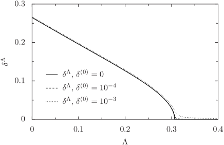
Figure 3: Flow of the superconducting gap $\delta^{\Lambda}$ for various values of the bare gap $\delta^{(0)}$.

The flow of the phase component of the Nambu vertex $\Phi^{\Lambda}$ is shown in the left panel of Fig. 4, and its final value at $\Lambda=0$ as a function of $\delta^{(0)}$ in the right panel. Note that $\Phi^{\Lambda}$ has the same shape as $\delta^{\Lambda}$, and that $\Phi^{\Lambda=0}$ diverges as $1/\delta^{(0)}$ for small $\delta^{(0)}$, as described by Eq. (74).

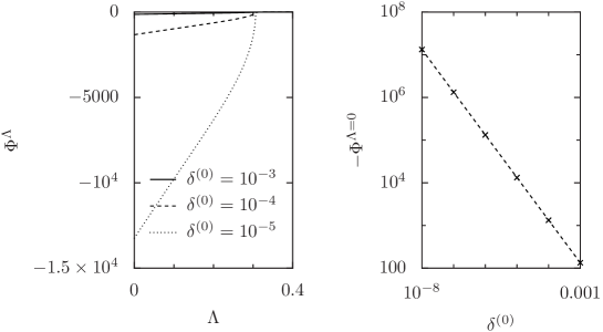
Figure 4: Left: Flow of the phase component of the Nambu vertex $\Phi^{\Lambda}$ for various values of $\delta^{(0)}$. Right: Phase component of the Nambu vertex at the end of the flow ($\Lambda=0$) as a function of $\delta^{(0)}$. Note that $\Phi^{\Lambda}$ is momentum independent due to the choice of a constant form factor $f_{sc}({\bf k})=1$.

In Fig. 5 we plot the flow of the amplitude component of the Nambu vertex $A^{\Lambda}$ and of the anomalous component related to (3+1)-interactions $X^{\Lambda}$. Both diverge at the critical scale $\Lambda_{c}$ for $\delta^{(0)}\to 0$, but decrease again for $\Lambda<\Lambda_{c}$. Note that $X^{\Lambda}$ is much smaller than $A^{\Lambda}$ for any $\Lambda$.

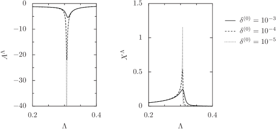
Figure 5: Flow of the amplitude component $A^{\Lambda}$ (left) of the Nambu vertex and of the anomalous component $X^{\Lambda}$ corresponding to (3+1)-interactions (right) for various values of $\delta^{(0)}$. Note that $A^{\Lambda}$ and $X^{\Lambda}$ are momentum independent due to the choice $f_{sc}({\bf k})=f_{c}({\bf k})=1$.

5 Channel decomposition

When solving the flow equation for the two-particle vertex for a realistic (not mean field) model, one faces the problem that rather complex momentum and frequency dependences are generated by the flow. In a translation invariant system, the two-particle vertex depends on three independent momentum and frequency variables. In previous works the frequency dependence was usually discarded, and the momentum dependence was crudely discretized.[3, 4, 5, 12] That procedure can be justified by power counting, as long as the flowing interactions remain weak and regular. However, in case of spontaneous symmetry breaking the two-particle vertex diverges in certain channels and singular momentum and frequency dependences develop.

In this section we present a first step toward an efficient parametrization of the two-particle vertex, which captures the singular momentum and frequency dependences associated with the flow into a superconducting phase. The singular momentum dependence of the vertices originates from that of the loop integrals in the RG equations. Therefore, we decompose the vertices into several interaction channels, with the purpose of isolating the singular momentum dependence of each diagram. Distributing the diagrams among the channels according to their momentum dependence then leads to channel-decomposed flow equations.

For the normal vertices, we follow the approach by Husemann and Salmhofer [13] and add several general two-particle interaction terms for the different channels to the bare interaction. The latter is not distributed among the channels to avoid ambiguities. The interaction channels then describe corrections to the bare interaction from integrating out modes in the functional integral. We make the ansatz

$$\Gamma^{(2+2),\Lambda}[\psi,\bar{\psi}] = V[\psi,\bar{\psi}]+\frac{1}{2}\sum_{k_{i},\sigma_{i}}\delta_{k_{1}+k_{2},k_{3}+k_{4}}$$ (77)

$$\times \left\{\left[V^{sc,\Lambda}_{k_{1},k_{4}}(k_{1}+k_{2})+V^{c,\Lambda}_{k_{1},k_{2}}(k_{3}-k_{2})\right]\delta_{\sigma_{1}\sigma_{4}}\delta_{\sigma_{2}\sigma_{3}}\right.$$

$$+\left.V^{s,\Lambda}_{k_{1},k_{2}}(k_{3}-k_{2})\left(2\delta_{\sigma_{1}\sigma_{3}}\delta_{\sigma_{2}\sigma_{4}}-\delta_{\sigma_{1}\sigma_{4}}\delta_{\sigma_{2}\sigma_{3}}\right)\right\}$$

$$\times \bar{\psi}_{k_{1}\sigma_{1}}\bar{\psi}_{k_{2}\sigma_{2}}\psi_{k_{3}\sigma_{3}}\psi_{k_{4}\sigma_{4}}\;,\hskip 22.76219pt$$

where $V[\psi,\bar{\psi}]$ is the bare interaction and the superscripts sc, $c$, and $s$ refer to ”superconducting”, ”charge”, and ”spin” channels, respectively. The momentum (and frequency) argument in parentheses is the total momentum of the interacting electrons for the superconducting channel and the momentum transfer for the charge and spin channels. These are the variables for which a singular dependence is expected. If the other momentum dependences remain regular, the above ansatz provides a good starting point for a parametrization of the various interaction channels as interactions mediated by a boson exchange.

After symmetrization and translation to Nambu notation, one of the Nambu components representing the (2+2)-interaction reads

$$\Gamma^{(4),\Lambda}_{+-+-}(k_{1},k_{2},k_{3},k_{4}) = V^{(0)}(k_{1},-k_{4},-k_{2},k_{3})+V^{sc,\Lambda}_{k_{1},k_{3}}(k_{3}-k_{2})+V^{c,\Lambda}_{k_{1},-k_{4}}(k_{1}-k_{3})$$ (78)

$$- 2V^{s,\Lambda}_{k_{1},-k_{4}}(k_{1}+k_{2})-V^{s,\Lambda}_{k_{1},-k_{4}}(k_{1}-k_{3})\;,$$

where $k_{4}=k_{1}+k_{2}-k_{3}$. Note that the total momentum of electrons in the superconducting channel has transformed to a momentum transfer in the Nambu representation, while the momentum sum $k_{1}+k_{2}$ now appears in one of the spin-channel terms.

The propagators in Eq. (10) transport the following momenta through the diagrams, which they depend on singularly:

$$\Pi^{PH,d}_{s_{1}s_{2}s_{3}s_{4}}(k_{1},k_{2},k_{3},k_{4}) : \;\mbox{momentum transfer }k_{3}-k_{2}\;,$$

$$\Pi^{PH,cr}_{s_{1}s_{2}s_{3}s_{4}}(k_{1},k_{2},k_{3},k_{4}) : \;\mbox{momentum transfer }k_{3}-k_{1}\;,$$

$$\Pi^{PP}_{s_{1}s_{2}s_{3}s_{4}}(k_{1},k_{2},k_{3},k_{4}) : \;\mbox{total momentum }k_{1}+k_{2}\;.$$

The three terms contributing to the flow of the two-particle vertex in Eq. (9) are distributed among the various interaction channels according to their momentum dependence. Hence we assign the direct Nambu particle-hole diagram to the superconducting channel, such that

$$\frac{d}{d\Lambda}V^{sc,\Lambda}_{k_{1},k_{3}}(q)=\Pi^{PH,d}_{+-+-}(k_{1},k_{3}-q,k_{3},k_{1}-q)\;,$$ (79)

where the dependence on $q=k_{3}-k_{2}$ is expected to be singular in the superconducting phase. The Nambu particle-particle diagram is assigned to the spin channel,

$$\frac{d}{d\Lambda}V^{s,\Lambda}_{k_{1},k_{3}}(p)=\frac{1}{4}\Pi^{PP}_{+-+-}(k_{1},p-k_{1},k_{3}+p,-k_{3})\;,$$ (80)

with $p=k_{1}+k_{2}$. The crossed Nambu particle-hole diagram determines the flow of the remaining two terms in Eq. (78), that is,

$$\frac{d}{d\Lambda}V^{c,\Lambda}_{k_{1},k_{2}}(q^{\prime})-\frac{d}{d\Lambda}V^{s,\Lambda}_{k_{1},k_{2}}(q^{\prime})=-\Pi^{PH,cr}_{+-+-}(k_{1},-k_{2}-q^{\prime},k_{1}-q^{\prime},-k_{2})\;,$$ (81)

with $q^{\prime}=k_{3}-k_{1}$. Using the above flow equation for $V^{s,\Lambda}$, this yields

$$\frac{d}{d\Lambda}V^{c,\Lambda}_{k_{1},k_{2}}(q^{\prime})=\frac{1}{4}\Pi^{PP}_{+-+-}(k_{1},q^{\prime}-k_{1},k_{2}+q^{\prime},-k_{2})-\Pi^{PH,cr}_{+-+-}(k_{1},-k_{2}-q^{\prime},k_{1}-q^{\prime},-k_{2})\;.$$ (82)

We have thus obtained flow equations for all three contributions $V^{sc,\Lambda}$, $V^{c,\Lambda}$, and $V^{s,\Lambda}$ to the normal interaction. These channel decomposed flow equations for the normal interaction are equivalent to those derived by Husemann and Salmhofer [13] in the $\psi$-representation.

For the channel decomposition of the anomalous vertices, we profit from the symmetries described in § 3. For the functions $X^{S,T}(k_{1},k_{2},k_{3},k_{4})$ parametrizing $\Gamma^{(3+1)}[\psi,\bar{\psi}]$ in Eq. (26), we expect a singular dependence on the variable $k_{2}+k_{3}$, which is the total momentum of the Cooper pair contained in $\Gamma^{(3+1)}[\psi,\bar{\psi}]$. We therefore write

$$X^{S,\Lambda}(k_{1},k_{2},k_{3},k_{4}) = X^{S,\Lambda}_{k_{1},k_{2}}(k_{2}+k_{3})\;,$$

$$X^{T,\Lambda}(k_{1},k_{2},k_{3},k_{4}) = X^{T,\Lambda}_{k_{1},k_{2}}(k_{2}+k_{3})\;,$$ (83)

where $k_{4}=k_{1}+k_{2}+k_{3}$. As a Nambu component representing the (3+1)-interaction we choose

$$\Gamma^{(4),\Lambda}_{++-+}(k_{1},k_{2},k_{3},k_{4}) = X^{\Lambda}(k_{1},k_{2},k_{3},k_{4})$$ (84)

$$= X^{S,\Lambda}_{k_{1},k_{2}}(k_{2}-k_{3})+X^{T,\Lambda}_{k_{1},k_{2}}(k_{2}-k_{3})$$

$$- X^{S,\Lambda}_{k_{2},k_{1}}(k_{1}-k_{3})-X^{T,\Lambda}_{k_{2},k_{1}}(k_{1}-k_{3})+2X^{T,\Lambda}_{-k_{3},k_{2}}(k_{1}+k_{2})\;,\hskip 22.76219pt$$

where now $k_{4}=k_{1}+k_{2}-k_{3}$. Comparing the momentum dependences with those of the bubbles, we assign

$$\frac{d}{d\Lambda}\left[X^{S,\Lambda}_{k_{1},k_{2}}(k_{2}-k_{3})+X^{T,\Lambda}_{k_{1},k_{2}}(k_{2}-k_{3})\right] = \Pi^{PH,d}_{++-+}(k_{1},k_{2},k_{3},k_{1}+k_{2}-k_{3})\;,$$ (85)

$$\frac{d}{d\Lambda}\left[X^{S,\Lambda}_{k_{2},k_{1}}(k_{1}-k_{3})+X^{T,\Lambda}_{k_{2},k_{1}}(k_{1}-k_{3})\right] = \Pi^{PH,cr}_{++-+}(k_{1},k_{2},k_{3},k_{1}+k_{2}-k_{3})\;,$$ (86)

$$\frac{d}{d\Lambda}X^{T,\Lambda}_{-k_{3},k_{2}}(k_{1}+k_{2}) = -\frac{1}{4}\Pi^{PP}_{++-+}(k_{1},k_{2},k_{3},k_{1}+k_{2}-k_{3})\,.\hskip 28.45274pt$$ (87)

Eqs. (85) and (86) are equivalent, since

$$\Pi^{PH,d}_{s_{1}s_{2}s_{3}s_{4}}(k_{1},k_{2},k_{3},k_{4})=\Pi^{PH,cr}_{s_{2}s_{1}s_{3}s_{4}}(k_{2},k_{1},k_{3},k_{4})\;.$$ (88)

Solving for $X^{S,\Lambda}$ and $X^{T,\Lambda}$, and relabeling variables, one obtains

$$\frac{d}{d\Lambda}X^{S,\Lambda}_{k_{1},k_{2}}(q) = \Pi^{PH,d}_{++-+}(k_{1},k_{2},k_{2}-q,k_{1}+q)+\frac{1}{4}\Pi^{PP}_{++-+}(q-k_{2},k_{2},-k_{1},k_{1}+q)\;,$$

$$\frac{d}{d\Lambda}X^{T,\Lambda}_{k_{1},k_{2}}(q) = -\frac{1}{4}\Pi^{PP}_{++-+}(q-k_{2},k_{2},-k_{1},k_{1}+q)\;.$$ (90)

For the anomalous (4+0)-interactions we expect a singular dependence on the momentum of each Cooper pair contained in $\Gamma^{(4+0)}[\psi,\bar{\psi}]$, Eq. (3), which leads us to the ansatz

$$W^{S,\Lambda}(k_{1},k_{2},k_{3},k_{4}) = W^{S,\Lambda}_{k_{1},-k_{3}}(k_{1}+k_{2})\;,$$

$$W^{T,\Lambda}(k_{1},k_{2},k_{3},k_{4}) = W^{T,\Lambda}_{k_{1},-k_{3}}(k_{1}+k_{2})\;,$$ (91)

where $k_{4}=-k_{1}-k_{2}-k_{3}$. The corresponding Nambu component becomes

$$\Gamma^{(4),\Lambda}_{++--}(k_{1},k_{2},k_{3},k_{4}) = W^{\Lambda}(k_{1},k_{2},k_{3},k_{4})$$ (92)

$$= W^{S,\Lambda}_{k_{1},k_{3}}(k_{3}-k_{2})+W^{T,\Lambda}_{k_{1},k_{3}}(k_{3}-k_{2})$$

$$- W^{S,\Lambda}_{k_{1},k_{4}}(k_{1}-k_{3})-W^{T,\Lambda}_{k_{1},k_{4}}(k_{1}-k_{3})+2W^{T,\Lambda}_{k_{1},k_{3}}(k_{1}+k_{2})\,,\hskip 28.45274pt$$

where $k_{4}=k_{1}+k_{2}-k_{3}$. Comparing once again the momentum dependences with those of the bubbles, we assign

$$\frac{d}{d\Lambda}\left[W^{S,\Lambda}_{k_{1},k_{3}}(k_{3}-k_{2})+W^{T,\Lambda}_{k_{1},k_{3}}(k_{3}-k_{2})\right] = \Pi^{PH,d}_{++--}(k_{1},k_{2},k_{3},k_{1}\!+\!k_{2}\!-\!k_{3})\;,$$ (93)

$$\frac{d}{d\Lambda}\left[W^{S,\Lambda}_{k_{1},k_{4}}(k_{1}-k_{3})+X^{T,\Lambda}_{k_{1},k_{4}}(k_{1}-k_{3})\right] = \Pi^{PH,cr}_{++--}(k_{1},k_{2},k_{3},k_{1}\!+\!k_{2}\!-\!k_{3})\;,$$ (94)

$$\frac{d}{d\Lambda}W^{T,\Lambda}_{k_{1},k_{3}}(k_{1}+k_{2}) = -\frac{1}{4}\Pi^{PP}_{++--}(k_{1},k_{2},k_{3},k_{1}\!+\!k_{2}\!-\!k_{3})\,,\hskip 28.45274pt$$ (95)

where Eqs. (93) and (94) are equivalent due to exchange symmetry. Solving for $W^{S,\Lambda}$ and $W^{T,\Lambda}$, and relabeling variables, one obtains

$$\frac{d}{d\Lambda}W^{S,\Lambda}_{k_{1},k_{2}}(q) = \Pi^{PH,d}_{++--}(k_{1},k_{2}-q,k_{2},k_{1}-q)+\frac{1}{4}\Pi^{PP}_{++--}(k_{1},q-k_{1},k_{2},q-k_{2})\;,$$

$$\frac{d}{d\Lambda}W^{T,\Lambda}_{k_{1},k_{2}}(q) = -\frac{1}{4}\Pi^{PP}_{++--}(k_{1},q-k_{1},k_{2},q-k_{2})\;.$$ (97)

So far no approximation has been made in rewriting the flow equations. Consequently, they capture the exact flow of the reduced (mean-field) model discussed in § 4. There, however, redundancies in the Nambu vertex for the reduced model could be exploited in order to construct the solution entirely in the momentum channel $k_{1}=k_{4}$, $k_{2}=k_{3}$, where the flow is determined exclusively by the direct Nambu particle-hole diagram.

The channel decomposition of the vertex and the flow equations provides a very useful starting point for an efficient approximate parametrization of the momentum and energy dependences being generated in the various channels in the course of the flow for models with generic interactions, as shown for the normal (not symmetry-broken) state of an interacting Fermi system by Husemann and Salmhofer.[13]

6 Conclusions

We have addressed the problem of finding an efficient parametrization for the effective two-particle vertex in a spin-singlet superconductor, with the perspective to solve functional renormalization group flow equations for interacting Fermi systems with a superconducting ground state. We have constructed a manifestly spin-rotation invariant form of the vertex, which reduces the number of independent Nambu components to only three functions ($V$, $W$, and $X$). By studying the exact flow of the vertex for a reduced (mean-field) model exhibiting superconductivity and also forward scattering, we have identified the singularities of the vertex associated with the superconducting instability. We have then expressed the vertex as a sum of various interaction channels where potential singularities are isolated in only one momentum and frequency variable in each channel, and derived the corresponding channel-decomposed flow equations.

Our work paves the way for a controlled solution of the rather complex flow equation governing the flow of an interacting Fermi system into a superconducting phase. Since singular dependences generated by fermion loops have been isolated in only one momentum and energy variable per channel, one can parametrize these singularities by a relatively simple ansatz with a tractable number of parameters.

References

- [1] W. Metzner, Prog. Theor. Phys. Suppl. 160, 58 (2005).
- [2] J. Berges, N. Tetradis, and C. Wetterich, Phys. Rep. 363, 223 (2002).
- [3] D. Zanchi and H. J. Schulz, Phys. Rev. B 61, 13609 (2000).
- [4] C. J. Halboth and W. Metzner, Phys. Rev. B 61, 7364 (2000).
- [5] C. Honerkamp, M. Salmhofer, N. Furukawa, and T. M. Rice, Phys. Rev. B 63, 035109 (2001).
- [6] T. Baier, E. Bick, and C. Wetterich, Phys. Rev. B 70, 125111 (2004).
- [7] M. C. Birse, B. Krippa, J. A. McGovern, and N. R. Walet, Phys. Lett. B 605, 287 (2005).
- [8] S. Diehl, H. Gies, J. Pawlowski, and C. Wetterich, Phys. Rev. A 76, 021602(R) (2007).
- [9] P. Strack, R. Gersch, and W. Metzner, Phys. Rev. B 78, 014522 (2008).
- [10] M. Salmhofer, C. Honerkamp, W. Metzner, and O. Lauscher, Prog. Theor. Phys. 112, 943 (2004).
- [11] R. Gersch, C. Honerkamp, D. Rohe, and W. Metzner, Eur. Phys. J. B 48, 349 (2005).
- [12] R. Gersch, C. Honerkamp, and W. Metzner, New J. Phys. 10, 045003 (2008).
- [13] C. Husemann and M. Salmhofer, Phys. Rev. B 79, 195125 (2009).
- [14] C. Wetterich, Phys. Lett. B 301, 90 (1993).
- [15] M. Salmhofer and C. Honerkamp, Prog. Theor. Phys. 105, 1 (2001).
- [16] A. A. Katanin, Phys. Rev. B 70, 115109 (2004).
- [17] For a thorough discussion of time reversal in many-body systems, see L. Bányai and K. El Sayed, Annals of Physics 233, 165 (1994).
- [18] R. Gersch, Ph.D. thesis, University Stuttgart (2007).