Frequency Resolved Spectroscopy of XB 1323$-$619 Using XMM-Newton data: Detection of a Reflection Region in the Disk

Abstract

We present the frequency resolved energy spectra (FRS) of the low-mass X-ray binary dipper XB 1323$-$619 during persistent emission in four different frequency bands using an archival $XMM$-$Newton$ observation. FRS method helps to probe the inner zones of an accretion disk. XB 1323$-$619 is an atoll source and a type-I burster. We find that the FRS is well described by a single blackbody component with kT in a range 1.0-1.4 keV responsible for the source variability in the frequency ranges 0.002-0.04 Hz, and 0.07-0.3 Hz. We attribute this component to the accretion disk and possibly emission from an existing boundary layer supported by radiation pressure. The appearance of the blackbody component in the lower frequency ranges and disappearance towards the higher frequencies suggests that it may also be a disk-blackbody emission. We detect a different form of FRS for the higher frequency ranges 0.9-6 Hz and 8-30 Hz which is modeled best with a power-law and a Gaussian emission line at 6.4${}^{+0.2}_{-0.3}$ keV with an equivalent width of 1.6${}^{+0.4}_{-1.2}$ keV and 1.3${}^{+0.7}_{-0.9}$ keV for the two frequency ranges, respectively. This iron fluorescence line detected in the higher frequency ranges of spectra shows the existence of reflection in this system within the inner disk regions. The conventional spectrum of the source also shows a weak broad emission line around 6.6 keV (Boirin et al. 2005). In addition, we find that the 0.9-6 Hz frequency band shows two QPO peaks at 1.4${}^{+1.0}_{-0.2}$ Hz and 2.8${}^{+0.2}_{-0.2}$ Hz at about 2.8-3.1 $\sigma$ confidence level. These are consistent with the previously detected $\sim$ 1 Hz QPO from this source (Jonker et al. 1999). We believe they relate to the reflection phenomenon. The emission from the reflection region, being a variable spectral component in this system, originates from the inner regions of the disk with a maximum size of 4.7$\times 10^{9}$ cm and a minimum size of 1.6$\times 10^{8}$ cm calculated using light travel time considerations and our frequency resolved spectra.

1 Introduction

XB 1323$-$619 is an X-ray burster that shows varying intensity dips that repeat with the orbital period. The source is discovered by Uhuru and Ariel V (Forman et al. 1978; Warwick et al. 1981) and the dips and bursts are recovered with EXOSAT (van der Klis et al. 1985; Parmar et al. 1989). The typical dips last about 30% of the orbital cycle, and the 0.3-12.0 keV intensity varies creating sharp deep features in time with about $\sim$70% decrease in the persistent emission count rate. The source is viewed at $i=$ 60–80^∘ (Frank et al. 1987). The dip recurrence interval is not precisely known, with the best measurement of 2.94(2) hr (Balucinska-Church et al. 1999). The source is found to have persistent $\sim$1 Hz quasi-periodic oscillations (QPOs) (Jonker et al. 1999).

A $BeppoSAX$ observation of XB 1323$-$619 between 1.0–150 keV reveals persistent emission of the source modeled by a cutoff power-law with $\alpha$ = $1.48\pm 0.01$ and $E{\rm{}_{cut}}$ = $44.1\,^{+5.1}_{-4.4}$ keV together with a blackbody with $kT$ = $1.77\pm 0.25$ keV (Balucinska-Church et al. 1999). A more recent $INTEGRAL$ time-averaged 4.0-200.0 keV spectrum (combined JEM-X and ISGRI spectra) of XB 1323$-$619 can be best fitted using a blackbody emission of $kT$ = $1.7\pm 0.3$ keV and a Comptonized plasma emission model (CompTT, Titarchuck 1994) of $kT$ = $196.4\pm 28.5$ keV with a seed in photon temperature of $0.4\pm 0.2$ keV, and a Compton optical depth to scattering of $\tau$ = 0.002-0.007 (Balman 2009). An $RXTE$ observation below 20 keV reveals a cutoff power-law with $\alpha$ = $1.23\pm 0.07$ and a blackbody with $kT$ = $1.36\pm 0.06$ keV for the persistent emission (Barnard et al. 2001). A recent $Suzaku$ observation between 0.8 and 70 keV has a non-dip spectrum consistent with a blackbody model of $kT$ = $1.35\pm 0.36$ keV and a power-law with an $\alpha$ = $1.67\pm 0.1$ (Balucinska-Church et al. 2009). Boirin et al. (2005) detect Fe XXV and Fe XXVI absorption features from this source using the same archival observation analyzed in this paper. They find changes in the properties of the Fe XXV and Fe XXVI absorption features from persistent to dipping intervals indicating the presence of less-ionized material in the line of sight during dips (ionization parameter $\xi$ decreases from log($\xi$) of $3.9\pm 0.1$ to log($\xi$) of $3.13\pm 0.07$). It is suggested that absorption lines in dipping low-mass X-ray binaries are a result of a circularly symmetric photoionized region on the outer disk and as the source is viewed from the absorber at all times, the variations in the ionization parameter of this region causes the different levels of dipping in these systems (see also Diaz-Trigo et al. 2006, 2009). Church et al. (2005) has studied the same data set as Boirin et al. (2005) using absorption line ratios of Fe XXV/Fe XXVI and curve of growth analysis leading to the conclusion that a collisionally ionized plasma with kT=31 keV can reproduce the absorption lines in the $XMM$-$Newton$ Spectra. As they find that this temperature is close to the accretion disk corona (ADC) temperature (they have calculated using the $BeppoSax$ spectrum), they propose that the absorption lines in dipping low-mass X-ray binaries are produced in the ADC and there is no need to invoke a separate location where a highly ionized absorber exists.

In this paper, we aim at deriving frequency resolved spectra of XB 1323$-$619 in an attempt to reveal different emission regions and absorbing regions in the system extracting the variable component of the emission spectrum as opposed to the non-variable component by the described method in the paper. We expect that this method should, also, reveal the location of the emitting and absorbing regions in similar (dipping) LMXBs.

2 Data and the Observation

The $XMM$-$Newton$ Observatory (Jansen et al. 2001) has three 1500 cm² X-ray telescopes each with an European Photon Imaging Camera (EPIC) at the focus; two of which have MOS CCDs (Turner et al. 2001) and the last one uses pn CCDs (Strüder et al. 2001) for data recording. Also, there are two Reflection Grating Spectrometers (RGS, den Herder et al. 2001) located behind two of the telescopes. We use an archival $XMM$-$Newton$ observation of XB 1323$-$619 with a duration of 50 ksec between 2003 January 29 09:05 UTC and 2003 January 29 28:58 UTC. A thin optical blocking filter was used with the EPIC Cameras. EPIC pn and MOS1 were operated in the timing mode whereas MOS2 was operated in the full window imaging mode. For the FRS calculations in our work, we used only the timing mode EPIC pn data which provides a time resolution of 30 $\mu$sec together with the highest sensitivity (i.e., count rate) and energy resolution among the EPIC CCDs. The EPIC pn timing mode is a mitigation for pile-up in high count rate sources and allow for pile-up free data for rates below 1500 c s^-1 compressing the data to a single one-dimensional row of length 4^′.4. We analyzed the pipeline-processed EPIC pn timing mode data using Science Analysis Software (SAS) version 8.0.5. Data for analysis (single- and double-pixel events, i.e., patterns 0–4 with Flag=0 option) were extracted from a rectangular region of 87^′′ wide column for the source and the background events were extracted whenever necessary from a source free zone normalized to the source extraction area (ie.e., same rectangular area). We calculated a conventional source spectrum using the SAS task ESPECGET which automatically creates a source spectrum, background spectrum, the ancillary response file and the energy response matrix. These files were later utilized to calculate the response files for the frequency resolved spectra as the spectra were derived with the method explained in the next section. In general, background subtraction was applied for the FRS since EPIC pn background contribution at frequencies 0.002-300 Hz would be negligible. In the analysis, only persistent emission (as opposed to dipping parts of the light curve) were used to calculate light curves for the FRS analysis. In order to filter the persistent emission user-defined good time intervals were created using thresholds on count rates resulting in an effective exposure of about 40 ksec. Data were also checked for flaring episodes (of the background) and type-I bursts of the source and all such occurrences were cleaned with the above procedure. We obtained an average count rate of 27.3$\pm$0.02 for the source with a maximum variation of 25$\%$ for the persistent emission. This was later used to calibrate systematic errors of 13$\%$ on the FRS spectral bins.

3 Analysis and Results

3.1 Frequency Resolved Spectra

In this work, the frequency resolved energy spectra were calculated following the prescription of Revnivtsev et al. (1999) and Gilfanov et al. (2003) where they applied this method to RXTE data of LMXBs. One assumes that the inverse Fourier Transform, the light curve, is a function of an energy dependent term and a time dependent term and the light curves at different energies are related by linear transformations. One allows for two components in the source emission spectrum, a constant non-variable part of the source emission and flux variations of the second variable component. Spectrum of the variable component is the frequency resolved spectrum, FRS. In order to calculate the FRS, we created power spectra (PSD–Power Spectral Density) in a certain range of energy channels (100-4095) of the $XMM$-$Newton$ EPIC pn data with a pre-determined binning of 50, 100 or 200 energy channels in the given range for 320-16 seconds time segments for each PSD. In each set of four frequency ranges, spectra were produced with the same channel binning and the duration for the PSD segments. Fast Fourier Transforms (FFT) were computed to derive the PSD adopting the normalization of Miyamoto et al. (1991)

$$P_{j}=2|A_{j}|^{2}/N_{ph}C\ \ \ \ \ \ A_{j}=\sum x_{n}e^{iw_{n}t_{n}}$$

. In this prescription, $t_{m}$ is the time label for each time bin, $x_{m}$ is the number of counts in these bins, $N_{ph}$ is the total number of photons in each light curve and C is the average count rate in each time segment used to construct PSD. The Miyamoto normalization is in units of (rms/mean)²/Hz measuring the variability amplitudes in different energies and can be integrated over different frequency range of interest. The top panel of Figure 1 shows the average PSD of the persistent emission light curve for the $XMM$-$Newton$ observation of XB 1323$-$619 computed using the Miyamoto normalization. Finally, for integrated frequency ranges of interest, the frequency dependent spectra can be constructed by

$$F(E_{k},f_{m})=C_{k}\sqrt{P_{k}(f_{j})\Delta f_{j}}$$

where F is the count rate of the spectrum on the frequency $f_{m}$ in the energy channel $E_{k}$.

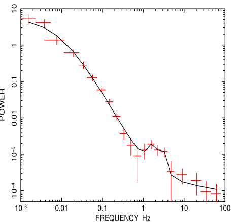
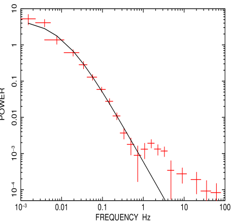
Figure 1: The average power spectrum (PSD) of XB 1323$-$619 using a Miyamoto normalization in units of (rms/mean)²/Hz. A certain white noise level is subtracted. The top panel is the PSD of the persistent emission data fitted with a composite model of three Lorentzians and a power-law model. The bottom panel shows the fit to the same PSD with a single Lorentzian displaying a high frequency excess.

We calculated FRS with the above method in four different frequency bands of 0.002-0.04 Hz, 0.07-0.3 Hz, 0.9-6 Hz, and 8-30 Hz. The frequency bands were selected according to the simple criteria that there is good statistics in the frequency range and the FRS produced have comparable count rates. We also used frequency ranges that complies with the different components of the PSD. Among these bands, 0.9-6 Hz frequency range (the two narrow Lorentzian components of the PSD as discussed below in the next section) includes the frequency of 1 Hz-QPO detected earlier from this system (Jonker et al. 1999).

3.2 The Average Power Spectrum and the Detected QPOs

We averaged several power spectra to create a PSD of XB 1323$-$619 using the Miyamoto normalization in units of (rms/mean)²/Hz. Figure 1 shows a fitted PSD with a composite model of three Lorentzians and a power-law following the prescriptions of Belloni, Psaltis, $\&$ van der Klis (2002), yielding a $\chi^{2}_{v}$ of 1.0 for 10 degrees of freedom (the white noise level is already subtracted). The bottom panel of Figure 1 displays the same PSD fitted by a single broad Lorentzian producing an unsuccessful fit with a $\chi^{2}_{v}$ value of 2.9 for 17 degrees of freedom. The very broad Lorentzian models the low frequencies. One of the narrow Lorentzians have a peak at 1.4${}^{+1.0}_{-0.2}$ Hz with a width of about 0.001 Hz. This is similar to the detected 1 Hz QPO from this system. The other narrow Lorentzian is at 2.8${}^{+0.2}_{-0.2}$ with a width of 0.003 Hz. The significance of the detected Lorentzians can be calculated following (Van der Klis, 1989 ; see also Boirin et al. 2000). We assume that SNR (in $\sigma$) = P_m-P_ref/E_P where P_m is the power at Lorentzian peak of interest, P_ref is the power of the continuum noise at the same peak frequency, and E_P is the error of the frequency bin at the Lorentzian peak. We note that the standard deviation of the average of the powers at the Lorentzian peak is taken as the error since it is larger and more representative rather than a theoretical estimation including power at the peak frequency and square root of the multiplication of the number of PSD averaged together and the number of raw frequency bins averaged together. We find that the significance of the 1.4${}^{+1.0}_{-0.2}$ Hz Lorentzian is at 2.8 $\sigma$ and the 2.8${}^{+0.2}_{-0.2}$ Hz Lorentzian is at 3.1 $\sigma$ confidence level, respectively. In addition, we calculate an integrated rms variability of 15$\%$ for the QPO at 1.4 Hz and 11$\%$ for the QPO at 2.8 Hz. Finally, the continuum of the high frequencies is best modeled using a power-law with an index of -0.4${}^{+0.2}_{-0.2}$.

3.3 Results of the FRS Analysis

The derived spectra (FRS) were fitted with a set of models comprising a combination of, or solely by, a power-law, a blackbody and a Gaussian emission line models, all absorbed by neutral matter with column density $N_{H}$ (these are POWER, BBODY, GAUSS, and WABS models within XSPEC, respectively). The fit parameters are displayed in Table 1. For the spectral analysis of the derived FRS, XSPEC version 12.5.1 has been used (Arnaud 1996). Spectral uncertainties are given at 90$\%$ confidence level ($\Delta$$\chi^{2}$= 2.71 for a single parameter). We grouped the FRS spectral energy channels in groups of 2-3 to improve the statistical quality of the spectra. During the entire fitting procedure a constant systematic error of 13$\%$ was used ( see sec. 2). The fits were conducted within 0.5-9.0 keV range. Figure 2 shows the fitted spectra in the four frequency bands. The conventional spectral analysis can be found in Boirin et al. (2005) and Church et al. (2005).

The results show that the best fitting model in the 0.002-0.04 Hz, and 0.07-0.3 Hz ranges, is a single blackbody (see Figure 2 top panels) with a $\chi^{2}_{v}$ value of 1.0 (see Table 1; The best fit results for each low frequency FRS are highlighted in bold-face) . The blackbody temperature is in a range 1.0-1.4 keV (90$\%$ confidence level errors). For the two low frequency ranges, the power-law (POWER) model or a power-law plus a Gaussian emission line (POWER+GAUSS) model fits yield $\chi^{2}_{v}$ values in excess of 4.0 for very similar degrees of freedom of 10-13. The fits with blackbody and a power-law (BBODY+POWER) or a combination of blackbody, power-law and a Gaussian emission line (BBODY+POWER+GAUSS) models yield similar $\chi^{2}_{v}$ values to blackbody (BBODY) fits. The added POWER model gives a power-law index which is unrealistically steep. Also, the included GAUSS model gives a normalization for the line of almost zero (see Table 1). Thus, we tested the significance of adding the power-law (POWER) and Gaussian emission line (GAUSS) models to the blackbody (BBODY) model using FTEST. The FTEST probability yields a value in a range of 0.40-0.46 for including the POWER and POWER+GAUSS models along with the blackbody model which is too high. As a result, we find that the BBODY+POWER or BBODY+POWER+GAUSS composite-model fits are redundant.

The other two FRS in the 0.9-6 Hz, and 8-30 Hz ranges were found to be consistent with each other and the fits were conducted simultaneously to increase the degrees of freedom. We find that the two FRS can be fitted best using a combination of a power-law and a Gaussian emission line (POWER+GAUSS) model with a $\chi^{2}_{v}$ of 1.1 for 8 degrees of freedom compared with any other model or combination of models (see Table 1; The best fit results for each high frequency FRS is highlighted in bold-face). An emission line at 6.1-6.6 keV (90$\%$ confidence level; best fit value is 6.4 keV) has been found necessary to improve the power-law fits (see Figure 2 bottom panels) . The bottom right-hand panel in Figure 2 shows the unfolded photon spectra and the line is clearly visible. This is the iron K_α fluorescence line indicator of reflection and/or reprocessing in the system dominating the variability at these frequencies. The width ($\sigma$) of the iron K_α line is $<$0.5 keV for the 0.9-6 Hz and 0.7${}^{+0.3}_{-0.5}$ keV for the 8-30 Hz ranges. The equivalent width of the line is large and it is 1.6${}^{+0.4}_{-1.2}$ keV for the 0.9-6 Hz and 1.3${}^{+0.7}_{-0.9}$ keV for the 8-30 Hz frequency bands, respectively. The fits with a single blackbody model, a single power-law model or a combination of the two (POWER+BBODY) yield unacceptable fits (see Table 1). On the other hand, a blackbody, power-law and Gaussian emission line (BBODY+POWER+GAUSS) composite model fit gives the same $\chi^{2}_{v}$ with the fitted POWER+GAUSS model (see Table 1). The blackbody temperature is 1.4-2.0 for this fit and the included blackbody model has a very low normalization in the spectra. We tested the significance of adding the BBODY model to the POWER+GAUSS model fit using FTEST. The FTEST probability yields a value of 0.42 for including the BBODY model along with the POWER+GAUSS model in the fitting procedure which is too high. Thus, a fit with a blackbody plus a power-law and a Gaussian emission line is redundant.

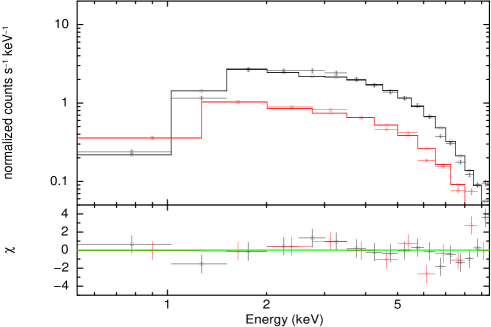
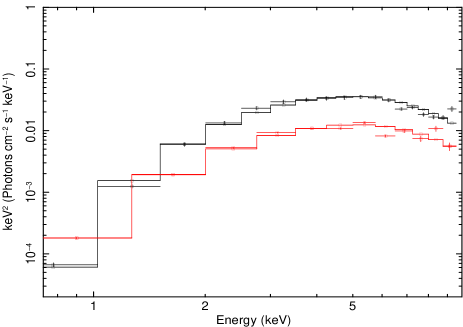
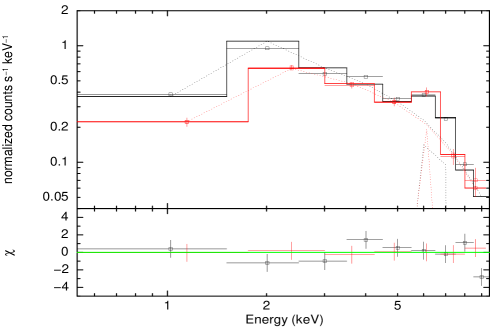
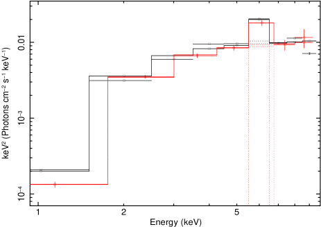
Figure 2: Frequency resolved energy spectra (FRS) of XB 1323$-$619 in four different frequency bands. The top two panels show the FRS fitted with a neural hydrogen absorption model (Galactic) and a blackbody model WABS$\times$BBODY (XSPEC models) of emission in the 0.002-0.04 Hz (the curve in black color), and 0.07-0.3 Hz (the curve in red color) frequency bands. The top left-hand panel is the count rate spectra and the top right-hand panel is the unfolded photon spectra in E²f(E) . The small panel under the count rate spectra shows the residuals in sigmas. The two bottom panels show the FRS fitted with a neural hydrogen absorption model (Galactic) and a power law with a Gaussian emission line model WABS$\times$(POWER+GAUSS) (XSPEC models) of emission in the 0.9-6 Hz (the bottom curve in red color) and 8-30 Hz (the top curve in black color) frequency bands. The bottom left-hand panel is the count rate spectra and the bottom right-hand panel is the unfolded photon spectra in E²f(E). The small panel under the count rate spectra shows the residuals in sigmas.

3.3.1 Statistical Significance of the 6.4 keV Fe Line

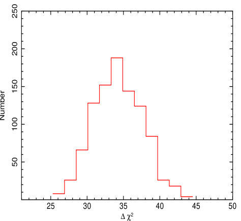
Figure 3: $\Delta\chi^{2}$ against cumulative number of chance of occurrences for adding a single Gaussian line in 1000 randomly simulated spectra. The null hypothesis spectra is a power-law with a neutral hydrogen absorption (Galactic). The $\Delta\chi^{2}$ values vary between 25 and 45 for 8 degrees of freedom. This line detection is over 99$\%$ confidence level in the frequency resolved spectra.

We carried out a detailed test of significance of existence of the Gaussian emission line using Monte Carlo simulations (e.g., Porquet et al. 2004; Minuitti & Fabian 2006). For our null, hypothesis, we assumed that the spectrum is simply an absorbed power-law continuum with the same parameters as the absorbed power-law model fitted to real data. We used the XSPEC FAKEIT command to create 1000 fake EPIC pn spectra corresponding to this model with photon statistics expected from $\sim$ 40 ksec exposure and grouped the spectra exactly as we have grouped the real spectra. Next, we fitted each fake spectrum using an absorbed power-law model with all parameters let to vary to obtain a $\chi^{2}$ value. We, then added a line, restricting the line with $\sigma$ between 0-1.0 keV in steps of 0.1 keV and, constraining the line energy between 6.0-7.5 keV with a step of 0.2 keV between each energy value and fitted the fake spectra, this time, with a composite model of a power-law plus a Gaussian line model (GAUSS+POWER). This resulted in 1000 simulations of $\chi^{2}$ values from each hypothesis. Then, the two $\chi^{2}$ values from each hypothesis were subtracted. The resulting distribution of $\Delta\chi^{2}$ against cumulative number of occurrences is displayed in Figure 3. The curve is a Gaussian centered on $\Delta\chi^{2}$$\sim$ 34.2 and varies between 25 and 45. The improvement in the $\chi^{2}$ value as calculated using the (POWER and POWER+GAUSS) model fits in Table 1 is 33 for 3 degrees of freedom. The probability that one gets a detection of a (false) Gaussian line in the fake data which gives an improvement in $\chi^{2}$ equal or better than that obtained in the real data is measured by integrating (counting the number of occurances) Figure 3 for $\Delta\chi^{2}$$\geq$ 33. This integration yields a probability of 0.002 implying that the line detection is over 99$\%$ confidence level and that the detection in our FRS is not by chance.

Table 1: Best-fit spectral parameters of FRS for the four different frequency ranges obtained using a power-law, a BBODY model or the combination of the two together with a neutral hydrogen absorption model WABS. Also, an additive Gaussian model is used. $N{\rm{}_{H}}$ is the absorbing column in units of $10^{22}$ atom cm^-2, $kT$ is the blackbody temperature in keV, $K{\rm{}_{B}}$ is the normalization of the blackbody model, $\Gamma$ is the power law photon index, $K{\rm{}_{pl}}$ is the model normalization photon cm^-2 s^-1 keV^-1 at 1 keV, $E_{0}$ is the central energy of the Gaussian model in keV, $\sigma$ is the width of the Gaussian line in keV, $K{\rm{}_{G}}$ is the normalization of the Gaussian line in total photons cm^-2 s^-1 keV^-1. The best fitting model to the data in each frequency range is highlighted in bold-face.

Model	Parameters	Frequency band of the spectra
		0.002-0.04 Hz	0.07-0.3 Hz	0.9-6.0 Hz	8.0-31.0 Hz
BBODY
	NH	0.4${}^{\bf+0.3}_{\bf-0.3}$	0.9${}^{\bf+0.3}_{\bf-0.3}$	0.9${}^{+0.8}_{-0.6}$	0.4${}^{+0.3}_{-0.3}$
	$kT_{\rm B}$	1.3${}^{\bf+0.1}_{\bf-0.1}$	1.2${}^{\bf+0.1}_{\bf-0.2}$	1.5${}^{+0.4}_{-0.2}$	1.5${}^{+0.2}_{-0.2}$
	$K{\rm{}_{B}}$	0.0003${}^{\bf+0.0001}_{\bf-0.0001}$	0.0009${}^{\bf+0.0002}_{\bf-0.0001}$	0.0003${}^{+0.0004}_{-0.0001}$	0.0004${}^{+0.0001}_{-0.0001}$
	$\chi^{2}_{v}$ (dof)	1.0 (12)	1.0 (13)	2.8 (11)	2.8 (11)
POWER
	NH	1.2${}^{+0.4}_{-0.4}$	2.5${}^{+2.5}_{-1.0}$	2.5${}^{+1.0}_{-0.8}$	1.5${}^{+0.5}_{-0.5}$
	$\Gamma$	1.7${}^{+0.6}_{-0.4}$	2.4${}^{+1.3}_{-0.9}$	1.5${}^{+0.4}_{-0.4}$	1.5${}^{+0.4}_{-0.4}$
	$K{\rm{}_{pl}}$	0.007${}^{+0.002}_{-0.001}$	0.06${}^{+0.01}_{-0.02}$	0.005${}^{+0.004}_{-0.002}$	0.007${}^{+0.002}_{-0.004}$
	$\chi^{2}_{v}$ (dof)	3.8 (12)	4.2 (13)	3.8 (11)	3.8 (11)
POWER+GAUSS
	NH	1.2${}^{+0.4}_{-0.4}$	2.2${}^{+1.9}_{-0.6}$	2.8${}^{\bf+0.6}_{\bf-0.8}$	1.8${}^{\bf+0.4}_{\bf-0.4}$
	$\Gamma$	1.8${}^{+0.5}_{-0.5}$	2.2${}^{+1.0}_{-0.6}$	1.8${}^{\bf+0.3}_{\bf-0.2}$	1.8${}^{\bf+0.3}_{\bf-0.2}$
	$K{\rm{}_{pl}}$	0.008${}^{+0.001}_{-0.002}$	0.04${}^{+0.01}_{-0.01}$	0.007${}^{\bf+0.004}_{\bf-0.002}$	0.007${}^{\bf+0.004}_{\bf-0.002}$
	$E_{0}$	6.4 (fixed)	6.4 (fixed)	6.4${}^{\bf+0.2}_{\bf-0.3}$	6.4${}^{\bf+0.2}_{\bf-0.3}$
	$\sigma$	0.2 (fixed)	0.2 (fixed)	$\bf<$0.5	0.7${}^{\bf+0.3}_{\bf-0.5}$
	$K{\rm{}_{G}}$	$<$0.0001	$<$2.5$\times$10-5	0.0003${}^{\bf+0.0001}_{\bf-0.0001}$	0.0003${}^{\bf+0.0001}_{\bf-0.0001}$
	$\chi^{2}_{v}$ (dof)	4.6 (10)	4.9 (11)	1.1 (8)	1.1 (8)
POWER+BBODY
	NH	0.7${}^{+1.2}_{-0.4}$	1.2${}^{+0.8}_{-0.2}$	2.3${}^{+0.5}_{-0.6}$	2.3${}^{+0.5}_{-0.6}$
	$\Gamma$	5.0${}^{+2.8}_{-2.8}$	9.9${}^{<}_{-6.3}$	4.0${}^{+2.2}_{-0.5}$	4.0${}^{+2.2}_{-0.5}$
	$K{\rm{}_{pl}}$	0.001${}^{+0.001}_{-0.0009}$	0.001${}^{+0.004}_{-0.0009}$	0.03${}^{+0.02}_{-0.01}$	0.03${}^{+0.02}_{-0.01}$
	$kT_{\rm B}$	1.2${}^{+0.1}_{-0.1}$	1.2${}^{+0.2}_{-0.2}$	1.5${}^{+0.06}_{-0.7}$	1.5${}^{+0.06}_{-0.7}$
	$K{\rm{}_{B}}$	0.0003${}^{+0.0001}_{-0.0001}$	0.0009${}^{+0.0002}_{-0.0001}$	0.0004${}^{+0.0004}_{-0.0003}$	0.0004${}^{+0.0004}_{-0.0003}$
	$\chi^{2}_{v}$ (dof)	1.0 (10)	1.0 (10)	3.8 (11)	3.8 (11)
POWER+BBODY+GAUSS
	NH	0.7${}^{+1.2}_{-0.4}$	1.2${}^{+0.8}_{-0.2}$	3.9${}^{+2.0}_{-0.6}$	3.9${}^{+2.0}_{-0.6}$
	$\Gamma$	4.0${}^{+3.4}_{-0.8}$	$<$9.6	2.1${}^{+0.3}_{-0.3}$	2.1${}^{+0.3}_{-0.3}$
	$K{\rm{}_{pl}}$	0.001${}^{+0.003}_{-0.0009}$	0.002${}^{+0.003}_{-0.001}$	0.01${}^{+0.02}_{-0.003}$	0.01${}^{+0.02}_{-0.003}$
	$kT_{\rm B}$	1.2${}^{+0.1}_{-0.2}$	1.1${}^{+0.2}_{-0.1}$	1.7${}^{+0.3}_{-0.2}$	1.6${}^{+0.4}_{-0.2}$
	$K{\rm{}_{B}}$	0.0003${}^{+0.0001}_{-0.0001}$	0.001${}^{+0.001}_{-0.0009}$	0.00008${}^{+0.00007}_{-0.000002}$	0.00009${}^{+0.00005}_{-0.00003}$
	$E_{0}$	6.4 (fixed)	6.4 (fixed)	6.5${}^{+0.2}_{-0.5}$	6.5${}^{+0.2}_{-0.5}$
	$\sigma$	0.2 (fixed)	0.2 (fixed)	$<$0.5	0.8${}^{+0.3}_{-0.6}$
	$K{\rm{}_{G}}$	$<$0.0003	$<$2.4$\times$10-5	0.0003${}^{+0.0002}_{-0.0002}$	0.0003${}^{+0.0002}_{-0.0002}$
	$\chi^{2}_{v}$ (dof)	1.0 (9)	1.0 (10)	1.1 (6)	1.1 (6)

4 Discussion

FRS technique is applied to Galactic black hole candidates (Revnivtsev et al. 1999; Gilfanov et al. 2003; Sobolewska & Zycki 2006; Reig et al. 2006) to neutron star LMXBs (Gilfanov & Revnivtsev 2005, Revnivtsev & Gilfanov 2006; Shrader, Reig & Kazanas 2007) and also to active galactic nuclei (Papadakis et al. 2005, 2006). The systematic application of this technique to Z sources in several different states of the sources yields soft and hard variable thermal components. The normalization of these components change with accretion rate and thus state of the source. The softer of the two blackbodies in question is identified with the accretion disk and the harder one with the boundary layer. Particularly QPOs from such systems at the horizontal and normal branch indicates a particular hard FRS revealing the expectations that the QPOs originate from the boundary layer. The temperature of the harder disk component is found to change slowly with luminosity, but the boundary layer temperature remains constant with frequency confirming that the boundary layer is dominated with radiation pressure. These components appear mostly in the relatively higher Fourier frequency ranges of spectra whereas the disk-blackbody components appear in the lower Fourier frequency ranges.

A systematic FRS analysis of an atoll source (4U 1728-34) performed by Shrader et al. (2007) shows that the island state of the source is dominated by a power law or a blackbody (kT = 1.4-1.7) plus a power law model that does not vary with Fourier frequency for 0.008-0.8 Hz, 0.8-8 Hz, and 8-64 Hz frequency ranges. They do not detect a resonance iron line around 6.4 keV in the FRS. The higher accretion rate states of the source at the lower banana and upper banana show only a harder blackbody with a temperature around kT = 2.0-2.2 keV indicating that at higher luminosities and accretion rates the variable spectral component is coming from the boundary layer only and is fairly constant in normalization and temperature across frequencies and different luminosities. Gilfanov et al. (2003) study the FRS of the atoll source 4U1608-52 in the frequency ranges corresponding to the frequency average spectrum, kHz QPOs and a 45 Hz QPO spectra. Their results show that the FRS is consistent with two components one of which is the emission from the boundary layer with kT=2.0-2.2 keV or a CompTT model of Comptonized plasma emission. However, they find that the QPO spectra are mainly consistent with 2.1-2.4 keV blackbody spectra revealing the radiation pressure dominated boundary layer emission.

Our results indicate a blackbody model of emission with kT=1.0-1.4 keV for the two lowest frequency ranges from 0.002 to 0.3 Hz. This is consistent with the findings of Shrader et al. (2007) in similar frequency ranges with this study. The conventional spectral analysis of the $XMM$-$Newton$ data shows the existence of a blackbody model of emission as the softer X-ray component with kT=0.92-1.2 keV (Boirin et al. 2005; Church et al. 2005) which is, then, a variable component in the spectrum of the source. However, we note that any FRS calculated in this work shows $F_{\rm FRS}$ $<$ 0.12$F_{x}$ where $F_{x}$ is the total X-ray flux inferred from conventional spectral analysis. The X-ray luminosity of XB 1323$-$619 (5.2$\times$10³⁶ erg s^-1; Boirin et al. 2005) corresponds to a mass transfer rate of 0.08$\dot{M}_{edd}$ (The distance is 10-20 kpc and $\dot{M}$ could be as high as 0.13$\dot{M}_{edd}$) . We suggest that this soft component originates in the boundary layer and is persistent over the two frequency ranges supported by radiation pressure as expected. In addition, $INTEGRAL$ (an average spectrum over two years, Balman 2009), $RXTE$ (Barnard et al. 2001) and $Suzaku$ (Balucinska-Church et al. 2009) spectral analysis indicate similar blackbody temperatures between 1.0-1.7 keV (overlapping within 95$\%$ confidence level error range) taken at different epochs and relatively different luminosities in a range 1-5.2$\times$10³⁶ erg s^-1. This supports the stability of an existing boundary layer emission (see also sec. 1). On the other hand, we need to stress that the appearance of blackbody emission in the low frequencies such as in this case is a typical feature of the FRS of Z sources (e.g., Gilfanov & Revnivtsev 2005) and the blackbody is, then, a disk-blackbody. However, a disk-blackbody with such temperatures would be atypically high for an Atoll source (like XB 1323$-$619) (e.g., Tarana, Bazzano $\&$ Ubertini 2008; Di Salvo et al. 2000).

We find a different form of FRS and hardening of the spectra in the two higher frequency ranges. The existence of a power-law spectra with an iron fluorescence K_α line at 6.4${}^{+0.2}_{-0.3}$ keV in the two frequency ranges 0.9-6 Hz and 8-30 Hz with the lowest normalization reveals reflection from a media located in the vicinity of the main source of emission. In the case for reflection from optically thick cold neutral medium, the main reflection features are a narrow unshifted iron fluorescence K_α line at 6.4 keV, an absorption edge at 7.1 keV and a reflected continuum emission peaked at 20-30 keV (Basko et al. 1974; George & Fabian 1991). However, deviations from this reflection model (e.g., broad lines and smeared edges) is detected in X-ray binaries indicating complicated ionization stages in or motion of the reflecting media (e.g., Miller 2007, Cackett et al. 2009a, 2009b, 2008; Reis, Fabian & Young 2009; di Salvo et al. 2009; Reynolds et al. 2010). The complicated modelling of these modified lines show a line centered mainly on 6.4 keV (errors in a range from 6.0 to 6.9 keV) with large broadening of the widths (equivalent widths in a range 50-400 eV) including extended red-wings due to general relativistic effects (i.e., redshifts) or Comptonization in a hot inner corona. In the case for XB 1323$-$619 the spectral parameters on Table 1 reveal that a cold/warm reflection model with the unshifted iron K${\alpha}$ line is plausible and in the 0.9-6 Hz range. However, we calculate a $\sigma$ $<$ 0.5 keV for the width of the iron fluorescence line in the 0.9-6 Hz range and a $\sigma$ of 0.7${}^{+0.3}_{-0.5}$ keV in the 8-30 Hz frequency band at a 90$\%$ confidence level. The error on the central energy of the line (i.e., 6.1-6.6 keV) and the large width of the line (particularly in the 8-30 Hz range) allows for shifted and broad resonance Fe line in the FRS, as well. We detect broadening of the line width with increasing frequency as was detected in the FRS analysis of Cyg X-1 by Revnivtsev et al. (1999). In general, the parameters of the line is similar to the modified 6.4 keV Fe fluorescence lines detected in other X-ray binaries.

We calculate that the neutral hydrogen absorption, also, increases by a factor of 3-4 in the spectra at the two high frequency ranges. This strongly suggests that the FRS method may have revealed the location of an absorbing medium in the persistent emission. Particularly, the 0.9-6 Hz FRS shows the highest absorption due to neutral Hydrogen as modeled in Table 1, but since the FRS have low spectral resolution, the true absorption may be of any kind, warm or cold.

An emission line at 6.6 keV is also detected in the conventional spectral analysis of the persistent spectrum (Boirin et al. 2005). The $XMM$-$Newton$ analysis reveals a weak broad line with a FWHM of 2.0${}^{+0.6}_{-0.4}$ keV. As mentioned in the above paragraphs processes like relativistic broadening, Compton Scattering, rotational velocity broadening may be the reason for this large line broadening. The maximum limits of the line width we calculate from the FRS are smaller than the FWHM derived from conventional spectral analysis. Since the line in the conventional spectrum is weak, it is sensitive to the choice of the continuum emission. However, the large FWHM is a strong indication that it may be a blending between the iron fluorescence lines originating from the different parts of the disk (i.e., inner and outer disk).

We believe that the two high frequency band spectra belong to the reflected emission and thus show a different spectra in comparison with the rest of the frequency bands that show blackbody emission from the disk. The conventional spectral analysis of the $XMM$-$Newton$ data shows a power-law emission component as the harder X-ray component with $\Gamma$=1.6-2.0 (Boirin et al. 2005; Church et al. 2005) which is consistent with our results.

We find that the PSD of the persistent emission shows two Lorentzian components around 1.4 and 2.8 Hz at about 99$\%$ confidence level. We belive this is consistent with the $\sim$ 1 Hz QPO previously detected from this system (Jonker et al. 1999). There has been two suggestions for the origin of the 1 Hz QPO: 1) quasi-periodic obscuration of the central source by a structure in the disk producing relatively energy-independent oscillations (Jonker et al. 1999); 2) global disk oscillations (Titarchuck & Osherovich 2000). Jonker et al. (1999) suggest that the QPO can not be explained with Compton scattering alone since that would result in strong energy dependence of the QPO which is inconsistent with their findings. They suggest that the relatively low energy dependence may arise in a model with an intermediate temperature structure containing hot and cold electrons combining Compton scattering with absorption. Quasi-periodic obscuration of the central source emission by an opaque medium, an orbiting bump on the surface of the disk, may cause the QPO. The QPO exists in the persistent emission, the dips and the bursts consistently revealing the connection to our work that the source emission is incident on a reflector carrying its signature. The high inclination angle of the system also plays an important role. The high frequency FRS (0.9-30 Hz) derived in this study supports this scenario for the QPOs, since FRS is best fitted with a power-law confirming the Comptonizing nature and the absorption is then supported by the existence of the 6.4 keV Fe K_α emission line and higher N_H parameter values from the fits. In the light of the spectral results, the QPOs, and the 6.4 keV Fe K_α emission line, we suggest that high frequency FRS relates directly to reflection/reprocessing and scattering in the disk and the frequency bands used to derive the FRS would yield a finite light crossing time of the reflector ${\tau}_{ref}$=l_ref/c, also indicating the location of this region within the disk. For f=1–30 Hz, l_ref is c/2$\pi$f yielding a maximum size of 4.7$\times$10⁹ cm for the reflector and a minimum size of 1.6$\times$10⁸ cm that would also denote a minimum observable inner disk size (the inner disk is at or closer than this limit). We suggest that the FRS method applied in this work have recovered the reflected component in the system that had not been found before by conventional methods.

XB 1323$-$619 exhibits iron Fe XXV and Fe XXVI absorption lines and the system is viewed relatively close to edge-on. In general, this is true for most of the dipping LMXBs. The conventional spectral analysis indicates a lack of orbital phase dependence of features except during dips suggesting that a highly-ionized absorber can be located in a thin cylindrical geometry around the compact object. This suggested location of the highly ionized absorber in LMXBs is mainly in the outer disk (Boirin et al. 2005; Diaz-Trigo et al. 2006). In comparison with this scenario, our FRS analysis indicates that there is an absorbing region which is associated with the reflection zone in the inner regions of the disk at 4.7-0.2$\times$10⁹ cm. However, we note that though we find an absorbing medium in the inner regions of the disk, we do not rule out another absorbing region (possibly highly ionized) which can exist somewhere in the outer disk. A different approach using dip-ingress timing for all the dipping LMXBs (Church $\&$ Balucinska-Church 2004) indicates existence of extended accretion disk coronae (ADCs) having radial extend typically 50000 km or 5-50$\%$ of the accretion disk radius (Balucinska-Church et al. 2009). The calculated size of an extended ADC in XB 1323$-$619 is $\sim$2.7$\times$10⁹ cm (Church $\&$ Balucinska-Church 2004) with a temperature of about 44 keV. $INTEGRAL$ results show a temperature of about 196 keV in 4-200 keV range ( Balman 2009) with an estimated location of a suggested ADC at r $<$ 1$\times$10⁹ cm. The assumed location of the ADC have some overlap with the reflection region size we calculated using our FRS. Then, the 6.4 keV line broadening and may be due to Comptonization in an ADC. We note that the size of the reflection region is 4.7-0.2$\times$10⁹ cm as mentioned above and the general relativistic effects are detected within 40-1$\times$10⁷ cm (e.g., Papitto et al. 2009; Cackett et al. 2009b; Reis et al. 2009) and may not explain the large equivalent widths and extended line widths. We note that (using the $INTEGRAL$ results) such a hot ADC may possibly show band limited noise effects in harder energies and at relatively higher frequencies than the ones studied in this work.

Finally, we stress that we do not recover any absorption features (i.e., lines) in the four FRS we have calculated in this study which may rule out the existence of a highly ionized absorber within the inner zones of the accretion disk. However, if there were narrow weak absorption lines restricted to width $\sigma$ $<$ 0.14 keV and equivalent widths $<$ 0.04 keV (Boirin et al. 2005), our crude spectral resolution might have missed them out since we detect a strong Fe fluorescence line at 6.4 keV.

5 Summary and Conclusions

We have analyzed the frequency resolved energy spectra (FRS) of the low-mass X-ray binary dipper XB 1323$-$619 during persistent emission in four different frequency bands using an archival $XMM$-$Newton$ observation. We recover two different continuum shapes for the four frequency ranges we have studied. We find that the FRS shows a single blackbody component with kT in a range 1.0-1.4 keV for the variability in the frequency ranges 0.002-0.04 Hz, and 0.07-0.3 Hz. We attribute this component to the accretion disk and possibly emission from an existing boundary layer supported by radiation pressure. On the other hand, we stress that the emergence of a blackbody component in the lower frequency ranges and disappearance towards the higher frequencies suggests that it may also be a disk-blackbody emission given the FRS properties derived for Z-sources. We find a different form of FRS for the frequency ranges 0.9-6 Hz and 8-30 Hz which is a power-law model together with a Gaussian emission line at 6.4${}^{+0.2}_{-0.3}$ keV with an equivalent width of 1.6${}^{+0.4}_{-1.2}$ keV and 1.3${}^{+0.7}_{-0.9}$ keV for the two frequency ranges, respectively. The width $\sigma$ of the line is $<$ 0.5 keV and 0.7${}^{+0.3}_{-0.5}$ for the 0.9-6 Hz and 8-30 Hz ranges. In addition, we recover different neutral hydrogen column density for the FRS derived in our work. The $N_{\rm H}$ is highest in the 0.9-6.0 Hz range with a value of 2.8${}^{+0.6}_{-0.8}$ $\times 10^{22}$ cm^-2 and is only slightly lower for the 8.0-30.0 Hz range, but lower by a factor of 3-4 in the 0.002-0.04 Hz and 0.07-0.3 Hz ranges. So, there is more associated absorption towards the inner disk and a distinct absorption difference for the two different continuum detected for the FRS. We find that the emission structure within the inner regions of the disk is such that there is either boundary layer emission and an embedded reflection region with higher absorption towards the inner regions or there is a reflection region and an ADC in the inner disk followed by a disk-blackbody towards the outer disk regions. The derived iron fluorescence line shows the existence of reflection/reprocessing in this system within the inner disk region. The size of the reflection region is in a range 4.7-0.16$\times 10^{9}$ cm assuming light travel times. We suggest that the FRS method applied in this work have recovered the reflected component in the system that had not been found before by conventional spectral methods. We stress that FRS can be used in this manner to find reflection components in other LMXBs where conventional spectra can not be adequate. Finally, we find that the 0.9-6 Hz frequency band shows two QPO peaks at 1.4${}^{+1.0}_{-0.2}$ Hz and 2.8${}^{+0.2}_{-0.2}$ Hz at about 2.8-3.1 $\sigma$ confidence level with integrated rms variability of 15$\%$ and 11$\%$, respectively. We relate the origin of the QPOs to the reflection phenomenon. The width of the 6.4 keV line increases with increasing frequency where the location, the QPOs are produced, is the outer most regions of the reflection zone with the least spread in the line and the highest $N_{\rm H}$, thus, possibly a cold reflection zone (i.e., region with large clumps).

References

- (1) Arnaud K. A., 1996, in ASP Conf. Ser. 101:Astronomical Data Analysis Software and Systems V, 17
- (2) Balucińska-Church M., Church M.J., Oosterbroek T., Segreto A., Morley R., Parmar A.N., 1999, A & A, 349, 495
- (3) Balucińska-Church M., Dotani T., Hirotsu T. & Church M. J., 2009, A & A, 500, 873
- (4) Balman Ş., 2009, AJ, 138, 50
- (5) Barnard R., Balucińska-Church M., Smale A. P. & Church M. J., 2001, A & A, 380, 494
- (6) Basko M. M., Sunyaev R.A., Titarchuk L.G., 1974, A & A, 31, 249
- (7) Boirin L., Mendez M., Diaz-Trigo M., Parmar A.N., Kaastra, J.S. 2005, A & A, 436, 195
- (8) Boirin L., Barret D., Olive J.F., Bloser P.F., Grindlay J.E. 2000, A & A, 361, 121
- (9) Cackett E.M., Miller J.M., Homan J., van der Klis M., Lewin W.H.G., Mendez M., Raymond J., Steeghs D., 2009, ApJ, 690, 1847
- (10) Cackett E.M., Altamirano D., Patruno A., Miller J.M., Reynolds M., Linares M., Wijnands R., 2009, ApJ, 694, L21
- (11) Cackett E.M. et al., 2008, ApJ, 674, 415
- (12) Church M.J., Reed D., Dotani T., Balucinska-Church M., Smale A., 2005, 359, 1336
- (13) Church, M. J., & Balucińska-Church, M. 2004, MNRAS, 348, 955
- (14) Diaz-Trigo M., Parmar A.N., Boirin L., Mendez M., Kaastra J.S., 2006, A & A, 445, 179
- (15) Diaz-Trigo M., Parmar A.N., Boirin L., Motch C., Talavera A., Balman Ş., 2009, A & A, 493, 1061
- (16) Forman W., Jones C., Cominsky L., Julien P., Murrey S., Peters G., Tannanbaum H., Giacconi R., 1978, ApJS, 38, 357
- (17) Frank J., King A.R., Lasota, J.P., 1987, A & A, 178, 137
- (18) George I. A., Fabian A.C., 1991, MNRAS, 1991
- (19) Gilfanov M., Revnivtsev M., Molkov S., 2003, A & A, 410, 217
- (20) Gilfanov M., Revnivtsev M., 2005, AN, 326, 812
- (21) den Herder J. W. et al., 2001, A & A, 365, L7
- (22) Jansen F. et al., 2001, A & A, 365, L1
- (23) Jonker P.G., van der Klis M., Wijnands, R. 1999, ApJ, 511, L41
- (24) van der Klis M., Jansen F., van Paradijs J., Stollman G., 1985, Space Sci. Rev., 1985, 30, 512
- (25) van der Klis M., 1989, in Timing Neutron Stars, edited by Ogelman, H. and Van den Heuvel, EPJ, NATO ASI C262, Kluwer Academic Publishers, p.27
- (26) Miller J. M., 2007, ARAA, 45, 441
- (27) Minuitti G. & Fabian G., 2006, MNRAS, 366, 115
- (28) Papadakis I.E., Kazanas D., Ayklas A., 2005, ApJ, 631, 727
- (29) Papadakis I.E., Ioannou Z., Kazanas D., 2006, AN, 327, 1047
- (30) Papitto A., di Salvo T., D‘Ai A., Iaria R., Burderi L., Riggio A., Menna M.T. & Robba N. R., 2009, A & A, 493, L39
- (31) Parmar A.N., Gottwald M., van der Klis M., van Paradijs J., 1989, ApJ, 338, 1024
- (32) Porquet D., Reeves J. N., Uttley P. & Turner T. J., 2004, A & A, 427, 101
- (33) Reig P., Papadakis I.E., Shrader C.R., Kazanas D., 2006, ApJ, 644, 424
- (34) Reis R.C., Fabian A.C. & Young A.J., 2009, MNRAS, 399, L1
- (35) Reynolds M., Miller J. M., Homan J., Miniutti G., 2010, ApJ, 709, 358
- (36) Revnivtsev M., Gilfanov M., Churazov E., 1999, A & A, 347, L23
- (37) Renvivtsev M., Gilfanov M., 2006, A & A, 453, 253
- (38) di Salvo T. et al., 2009, MNRAS, 398, 2022
- (39) di Salvo T., Iaria R., Burderi L. & Robba N.R., 2000, ApJ, 542, 1034
- (40) Shrader C. R., Reig, P., Kazanas, D., 2007, ApJ, 667, 1063
- (41) Sobolewska M.A., Zycki P.T., 2006, 530, 955
- (42) Strüder L. et al., 2001, A & A, 365, L18
- (43) Tarana A., Bazzano A. & Ubertini P., 2008, ApJ, 688, 1295
- (44) Titarchuck L., 1994, ApJ, 434, 313
- (45) Titarchuck L., Osherovich V., 2000, ApJ, 542, L111
- (46) Turner M.J.L. et al., 2001, A & A, 365, L27
- (47) Warwick R.S. et al., 1981, MNRAS, 197, 865